University of Windsor University of Windsor
Scholarship at UWindsor
Scholarship at UWindsor
Electronic Theses and Dissertations Theses, Dissertations, and Major Papers
2012
Discovering Influential Nodes from Social Trust Network
Discovering Influential Nodes from Social Trust Network
Sabbir Ahmed University of Windsor
Follow this and additional works at: https://scholar.uwindsor.ca/etd
Recommended Citation Recommended Citation
Ahmed, Sabbir, "Discovering Influential Nodes from Social Trust Network" (2012). Electronic Theses and Dissertations. 5407.
https://scholar.uwindsor.ca/etd/5407
Discovering Influential Nodes from Social
Trust Network
By
Sabbir Ahmed
A Thesis
Submitted to the Faculty of Graduate Studies through the School of
Computer Science in Partial Fulfillment of the Requirements for the Degree
of Master of Science at the
University of Windsor
Windsor, Ontario, Canada
2012
Discovering Influential Nodes from Social
Trust Network
By
Sabbir Ahmed
APPROVED BY:
Dr. Eugene H. Kim, External Reader Department of Physics
Dr. Alioune Ngom, Internal Reader School of Computer Science
Dr. Christie I. Ezeife, Advisor School of Computer Science
AUTHOR’S DECLARATION OF ORIGINALITY
I hereby certify that I am the sole author of this thesis and that no part of this thesis has been published or submitted for publication.
I certify that, to the best of my knowledge, my thesis does not infringe upon anyone’s copyright nor violate any proprietary rights and that any ideas, techniques, quotations, or any other material from the work of other people included in my thesis, published or otherwise, are fully acknowledged in accordance with the standard referencing practices. Furthermore, to the extent that I have included copyrighted material that surpasses the bounds of fair dealing within the meaning of the Canada Copyright Act, I certify that I have obtained a written permission from the copyright owner(s) to include such material(s) in my thesis and have included copies of such copyright clearances to my appendix.
ABSTRACT
The goal of viral marketing is that, by the virtue of mouth to mouth word spread, a small set of influential customers can influence greater number of customers. Influence maximization (IM) task is to discover such influential nodes (or customers) from a social network. Existing algorithms adopt Greedy based approaches, which assume only positive influence among users. But in real life network, such as trust network, one can also get negatively influenced.
In this research we propose a model, called T-GT model, considering both positive and negative influence. To solve IM under this model, a trust network where relationships among users are either ‘trust’ or ‘distrust’ is considered. We first compute positive and negative influence by mining frequent patterns of actions performed. Then using local search a new algorithm, called MineSeedLS, is proposed. Experimental results on real trust network shows that our approach outperforms Greedy based approach by almost 35%.
KEYWORDS
DEDICATION
ACKNOWLEDGEMENT
My sincere appreciation goes to my parents, wife and siblings. Your perseverance and words of encouragement gave me the extra energy to see this work through.
I will be an ingrate without recognising the invaluable tutoring and supervision from Dr. Christie Ezeife. Your constructive criticism and advice at all times gave me the needed drive to successfully complete this work. The research assistantship positions helped as well!!
Special thanks go to my external reader, Dr. Eugene H. Kim, my internal reader, Dr. Alioune Ngom for accepting to be in my thesis committee. Your decision, despite your tight schedules, to help in reading the thesis and providing valuable input is highly appreciated.
TABLE OF CONTENT
AUTHOR’S DECLARATION OF ORIGINALITY ... III
ABSTRACT ... IV
DEDICATION... V
ACKNOWLEDGEMENTS ... VI
LIST OF FIGURES ... IX
LIST OF TABLES ... XI
CHAPTERS
1. INTRODUCTION... 1
1.1 Social Network Analysis ... 1
1.2 Data Mining ... 4
1.3 Social Network Graph and Properties ... 8
1.4 Social Network mining and challenges ... 14
1.5 Submodular Function Maximization ... 17
1.6 Influence Maximization ... 19
1.7 Thesis contribution ... 25
2. RELATED WORKS ... 28
2.1 Diffusion Models ... 28
2.1.1 Linear Threshold Model ... 29
2.1.2 Independent Cascade Model ... 32
2.2 Greedy algorithm for Influence Maximization ... 33
2.3 ‘Lazy Forward’ Optimization ... 39
2.4 Improving scalability of Greedy ... 42
2.4.1MixedGreedy ... 42
2.4.2 CELF++ ... 42
2.4.3 SimPath ... 43
2.4.4 Community Based Greedy ... 43
2.4.5 Sparsification of Influence Network ... 44
2.5 Data Mining Approaches ... 45
2.5.1Mining Action Log ... 46
2.5.3 Learning Influence Probability ... 51
3. PROPOSED MINING FOR INFLUENTIAL NODES FROM TRUST NETWORK ... 56
3.1 Trust-General Threshold Model ... 56
3.2 Solution framework ... 62
3.3 Computing Positive and Negative Influence Probability ... 66
3.4 Discovering Influential Nodes ... 68
3.5 Complexity Analysis ... 76
3.6 Running Example ... 76
3.6.1 Example Dataset ... 76
3.6.2 Preprocessing Step ... 79
3.6.3 Computing Influence Probability using APG ... 80
3.6.4 Mining Influential Nodes using mineSeedLS... 84
4. EXPERMENTS AND ANALYSIS ... 87
4.1 Dataset ... 87
4.1.1 Epinions Dataset ... 87
4.1.2 Wikipedia Dataset ... 88
4.2 Performance Analysis ... 88
4.3 Runtime Analysis ... 91
4.3.1 Runtime of APG ... 91
4.3.2 Runtime of mineSeedLS ... 91
5. CONCLUSIONS AND FUTURE WORKS ... 93
BIBLIOGRAPHY ... 94
LIST OF FIGURES
Figure 1: Data Mining process ... 4
Figure 2: An example of a decision tree ... 6
Figure 3: A clustering example ... 7
Figure 4: Example of Directed and Undirected Graph ... 9
Figure 5: Graph model of social network data in Table 3 and 4. ... 10
Figure 6: An example of Social Network Graph ... 11
Figure 7: Trust Network Graph ... 14
Figure 8: Types of Social Network Mining Tasks ... 14
Figure 9: Greedy algorithm requires Social network graph with influence probabilities 22 Figure 10: a) Social Network Graph. b) Action Log ... 24
Figure 11: Proposed framework by Goyal et al. (2010) ... 25
Figure 12: Linear Threshold Model example ... 31
Figure 13: Independent Cascade Model example ... 33
Figure 14: Social Network Graph modeled on data in table 5 ... 35
Figure 15: The Greedy k-best influence maximization algorithm ... 36
Figure 16: Running time of exhaustive search, greedy and CELF. ... 40
Figure 17: (a) Example social graph; (b) A log of actions; (c) Propagation graph of action a and (d) of action b ... 47
Figure 18: The propagation graph of an action PG(a) in fig.(a), Inf8(u4, a) in fig.(b), Inf8(u2, a) in fig.(c) ... 48
Figure 19: Compute Influence Matrix. (Goyal et al. 2008). ... 50
Figure 20: (a) Undirected social graph containing 3 nodes and 3 edges with timestamps when the social tie was created; (b) Action Log ... 53
Figure 21: Propagation graphs of actions in action log of Figure 20 b ... 54
Figure 22: Example of social network graph with influence probability ... 58
Figure 23: Trust- Influential Node Miner Framework ... 63
Figure 24: Trust based Influential Node Miner (T-IM) algorithm ... 64
Figure 25: The Preprocess() method.. ... 65
Figure 27: An example input to APG algorithm ... 66
Figure 28: Algorithm: Action Pattern Generator (APG) ... 67
Figure 29: Algorithm: SpreadTGT (G(V,E),S,TM,IM) ... 72
Figure 30: Algorithm: SpreadTGT2 (T, G(V,E),S,TM,IM) ... 73
Figure 31: Algorithm mineSeedLS() ... 75
Figure 32: Social network graph modelled from trust data in table 7. ... 80
Figure 33: Influence spreads of different algorithms on Wikipedia Dataset under TGT model... 90
Figure 34: Influence spreads of different algorithms on Epinions Dataset under TGT model... 90
Figure 35: Runtime of APG with various size of Action Log. ... 91
Figure 36: Running time on Epinion Dataset under TGT model. ... 92
LIST OF TABLES
Table 1:An example of a training set for classification ... 5
Table 2:An example of transaction table ... 8
Table 3: Sample table with user information ... 10
Table 4: Relationship information of users in Table 1 ... 10
Table 5: Sample social network data with Influence Probability ... 35
Table 6: Sample Influence Matrix ... 50
Table 7: Example of Trust Data. ... 77
Table 8: Example of an Action Log. ... 78
Table 9: Trust Matrix. ... 79
Table 10: Action sequence table of action log in table 8.. ... 81
Table 11: Values of Au for all user v in G(V,E). ... 81
Table 12: Au.vcomputed from action sequence table. ... 82
Table 13: A′u.vcomputed from action sequence table. ... 83
Table 14: Influence Matrix. ... 83
Table 15: Nodes with its joint influence probability in queue T. ... 84
Table 16: Nodes with its joint influence probability in queue T. ... 85
Table 17: Spread of each node. ... 86
Table 18: Epinions trust dataset. ... 87
CHAPTER 1
INTRODUCTION
1.1 Social Network Analysis
A social network is a social structure made up of individuals or entities (e.g. organization) also called "nodes", which are inter connected by various types of relationships, such as friendship, trust etc. Social Network Analysis (SNA) concentrates on techniques to analyze these relationships and information flows, between nodes in a social network, and produce formal models which facilitates understanding of the structure of a network as well as which network structure is more likely to emerge (Wellman and Berkowitz, 1988).
Popularity of online social networking sites (e.g. Facebook, Google+), caused a rise of social network data of very large scale. Researchers are actively involved in studying and understanding properties and structures of these networks and the challenges they pose by applying various data mining and machine learning methods to these data, such as Kempe et al (2003) and Leskovec et al. (2010). These studies are to better understand the online social structure, its growth and user behaviour etc. (Backstorm et al. 2010). Such studies can help developers of social network sites to improve user experience, make it scalable, and of course, profitable. Also tools and techniques for analysing and mining social network have various range of use in business processes such as marketing, sales etc. (Bonchi et al. 2011).
social network, or it can be a new technology, such as new android phone, a company wants to promote etc. Kempe et al. (2003) defines the influence maximization problem as a submodular function maximization problem and provide greedy based solution for it. Existing algorithms for influence maximization, such as Greedy (Kempe et al. 2003) and ‘Lazy Forward’ (Leskovec et al. 2006) based algorithms, requires that the influence probability, the probability of an individual adopting a product under the influence of another user, is known and given to the algorithm as input along with a social network graph. A social network graph can be easily constructed if the relationship (among users in a social network) data is explicitly available. However influence probabilities are not explicitly available (Goyal et al. 2008). In most of the literature reviewed influence probabilities are assumed and given as input.
In this research a trust network is considered, which is a social network where we have both positive (e.g. friendship) and negative (e.g. foes) types of links or edges, to solve influence maximization where both positive and negative influence exist. We propose a new model; called Trust-General Threshold (TGT) Model, in which the probability of a user to adopt a product relies on both positive and negative influence probabilities. By extracting patterns of actions performed by users we present a pattern mining based method to compute the influence probabilities (both positive and negative), from Action Log using Bernoulli distribution. Furthermore we show that, influence maximization under the new TGT model cannot be solved with good approximation guarantee using existing methods, such as ‘Lazy Forward’ of Leskovec et al. (2006). This is mainly because existing works assume that probability of a user performing an action increases as more of its neighbours perform the same action. However in our model this is not that case as the probability may in fact decrease if its neighbours who perform the actions are not the trusted ones. Using local search techniques we propose a new algorithm, MineSeedLS, to solve IM under TGT model. We conduct experiments using dataset collected from Epinions.com and Wikipedia.com to evaluate our approach.
1.2 Data mining
Data mining (also refer to as knowledge discovery from data or KDD) is the process of analysing data from different perspective and presenting it into meaningful information that can be used to make important and critical decisions. Agrawal and Srikant (1996) define data mining as a way of efficiently discovering interesting rules from large databases. This area of study is motivated by the need for solutions to decision support problems faced by organisations such as Banks, Retail stores etc.
Figure 1: Data mining process. (http://docs.oracle.com)
the mining task are accurate. The process of discovering interesting information from large set of data often employs different techniques and approaches. Some of the approaches include:
• Classification – it is the task of assigning or classifying objects to one of several
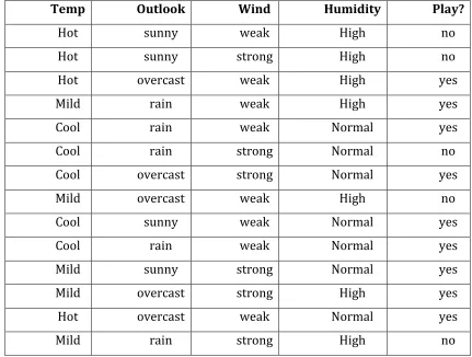
predefined categories or class. For example we may want to predict whether it is suitable to play tennis on a given day by looking into playing condition data from previous days. A collection of records, also known as training set, with their class labels is used as input data for a classification task. An example of an data of tennis play which can be used as training set for classification is in table 1 below:
Table 1: An example of a training set.
Temp Outlook Wind Humidity Play?
Hot sunny weak High no
Hot sunny strong High no
Hot overcast weak High yes
Mild rain weak High yes
Cool rain weak Normal yes
Cool rain strong Normal no
Cool overcast strong Normal yes
Mild overcast weak High no
Cool sunny weak Normal yes
Cool rain weak Normal yes
Mild sunny strong Normal yes
Mild overcast strong High yes
Hot overcast weak Normal yes
Mild rain strong High no
is called dependent attribute. The goal of any classification algorithm is to take training set data as input and produce a classification model which is then used to classify a new record of which the class or value for dependant attribute is unknown. Examples include decision tree classifiers, neural networks, naïve Bayes classifier etc. Figure 2 is a decision tree generated using the training set in table 1 above. A decision tree is a tree representation which is a collection of classification rules, one for each leaf node. In order to predict or classify an unknown record, the attribute values of the record are compared against the decision tree. A path from root of the decision tree to a leaf node which holds the predicted class of that record is traced.
Figure 2: An example of a decision tree.
The decision tree is then used to predict the value of the target attribute ‘play?’ for a new instance. For example, from the above decision tree model, if outlook is ‘sunny’ and humidity is ‘high’ we can predict ‘no’ for ‘play?’ attribute according to the decision tree.
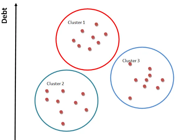
• Clustering – tasks seeks to discover records that are closely related and put them
algorithm is an example of a clustering algorithm. Figure 3 below shows a simple example of clusters of 3 groups separated based on debt and income.
Figure 3: A clustering example.
• Association rule mining – is used to discover patterns that describe strongly
bread and milk. The goal is to generate all possible patterns from the database, calculating their support (how often does the rule apply) and confidence (how often is the rule correct). Rules are generally simple, example, “If bread is purchased, then milk is purchased 60% of the time and this pattern occurs in 60% of all shopping baskets.”
Table 2: Example of transaction table
TID Items
1 {bread, milk}
2 {bread, diapers, beer, eggs} 3 {bread, diapers, beer, cola} 4 {bread, milk, diapers, beer} 5 {bread, milk, diapers, cola}
1.3 Social Network Graph and Properties
Graphs are used to specify relationships among a collection of items or nodes. It consists of a set of objects, called nodes, with certain pairs of these objects connected by links called edges. Graphs appear in many domains and context, whenever it is useful to model how things (or nodes) are either physically or logically connected to each other in a network structure (Easley and Kleinberg, 2010).
Following is the more formal definition of graph:
Definition 1 Graph - Graph G is a pair (V,E), where V is a set of vertices (or Nodes), and E is a set of edges between the vertices E⊆ {(u,v) | u, v ∈ V}
symmetric (e.g. friendship); the edge simply connects them to each other. However in various other settings, it may be required to express asymmetric relationships. For example a node can point to another node but not vice versa. Such relationships in a social network are modeled as directed graph which consist of a set of nodes with a set of directed edges; that is each directed edge is a link from one node to another. For example in Email network we need to specify sender and receiver. An example of a directed graph is shown in figure 4(b), with edges represented by arrows.
u1 u5
u2
u4
u3
u1 u5
u2
u4
u3
a) Undirected graph b) Directed graph
Figure 4 – Example of Directed and Undirected Graph.
(Easley and Kleinberg 2010). Let us consider the following social network data tables. Table 3 consist of list of individuals in a social network and Table 4 reports friendship relationship among these individuals.
Table 3: Sample table with user information
Userid Name Age Sex Location
101 Bob 32 M Toronto
102 Mary 22 F Windsor
201 Tanya 32 F Dhaka
301 Ahmed 22 M NewYork
Table 4: Relationship information of users in Table 3
Userid Friend_Of DateCreated
101 301 12-Mar-2007
301 201 22-Apr-2009
101 102 05-Jun-2011
102 301 02-Dec-2010
Based on these data we can model a simple social network graph as shown in Figure 5.
Figure 5 - Graph model of social network data in Table 3 and 4. Tanya
Ahmed Bob
In the above graph G(V,E), V is the set of individuals (or vertices) in the social network , i.e. V={Tanya, Bob, Ahmed, Mary}. And E is the set of all friendship links (or edges), i.e. E={(Tanya, Ahmed), (Bob, Mary),(Mary, Ahmed),(Bob, Ahmed)}.
Figure 6 - An example of Social Network Graph (Easley and Kleinberg, 2010. Page 48)
After modeling network data into graph, as shown in figure 6, social network mining tasks, such as (Kunegis et al. 2009), uses various graph based proximity measures, adapted from graph theory (Karamon et al. 2008). Following are some of the most commonly used graph-based properties used in mining and analysing network data. We use the example graph in figure 6 to explain these properties. The graph in figure 6 have 7 vertices as follows, V={A,B,C,D,E,F,G} and 8 edges as follows, E={(A,B), (A,D), (A,C), (A,E), (F,E), (F,B), (G,B)}.
a. Degree
b. Bridge
An edge is called a bridge if deleting the edge would cause its nodes at each endpoints to lie in different connected components of a graph. For example the edge GB in figure 4 is a bridge because it will split the graph into two connected components.
c. Distance
The distance between two vertices in a graph (denoted as dxy, the distance between node x and y) is the number of edges in a shortest path connecting them. For example the distance between nodes E and C in figure 6 is 2.
d. Closeness
Average distance from a node to all others. Closeness of node x can be calculated using following formula:
∑𝑦∈𝑉𝑑𝑥𝑦 𝑁 −1
Where N is the number of nodes in G (V, E)
e. Common Neighbours
For a node x, let Γ(𝑥) denote the set of neighbours of x in a social network graph. Common neighbours define CN(x, y) as the number of neighbours that x and y have in common:
𝐶𝑁(𝑥,𝑦) =Γ(𝑥)∩ Γ(𝑦)
For example number of common neighbours of nodes A and B in figure 6 is 1 (node D).
f. Clustering Coefficient
number of neighbours of vertex v. Then there is at most Kv * (Kv - 1)/2 number of
edges that can exist between the neighbours of v. If Lv is the number of edges that
actually exist between neighbours of v then clustering coefficient of node v, denoted as C(v)is:
𝐶(𝑣) = 𝐾 𝐿𝑣
𝑣∗(𝐾𝑣−1)/2
For example, the clustering coefficient of node A in figure 6 is 1/6. Because number of neighbors of A is 4, so number of edges that can exist between it’s neighbors is 4*(4-1)/2 = 6. And there is only one edge C-D among these possible six pairs.
Types of Social Network
The following are some of the main types of large-scale social networks that researchers have used for research in mining social network:
a. Friendship Network:
This is the simplest but most popular type of social network. Friendship network records who is friend to whom relationship among nodes. The largest of such network in online domain is currently Facebook which recently reported over 750 million users.
b. Collaboration Network:
Collaboration Network records who works with whom in a specific setting. Co-authorships among scientists, is an example of collaboration network. That is if 2 authors, A and B, publish a paper together there will be an edge between A and B in the corresponding Collaboration network.
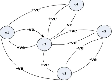
c. Trust Network
of others (Leskovec et al. 2010a, 2010b). Figure 7 below is a graph model of a typical trust network. u1 u5 u2 u4 u3 -ve +ve +ve -ve -ve +ve -ve -ve +ve +ve -ve
Figure 7 – A Trust Network graph example
d. Communication Network
Communication network models the “who-talks-to-whom” structure of social network. Such networks can be constructed from the logs of e-mail or from phone call records.
1.4 Social Network mining and Challenges
Data mining, such as classification, is very commonly used to tackle many SNA tasks and can be classified into two major categories; either descriptive or predictive (Figure 8).
Figure 8 – Types of Social Network Mining Tasks Data Mining of Social Network
Predictive
E.g. Link Prediction, Edge Sign Prediction etc.
Uses data mining such as Classification etc.
Descriptive
E.g. Group Detection, Discovery of Influential
Leaders etc. Uses data mining such as
A predictive model produced using mining social network data makes a prediction about unknown values. For example Prediction whether an individual will be a friend of another individual. This task is also known as Link Prediction (Liben-Knowell and Kleinberg, 2003). Classification and Regression are commonly used to produce predictive model in Social Network. Some predictive mining of social network are listed below:
a. Link Prediction
Link prediction task in social network is to predict existence of an edge between two nodes. More formally given a snapshot of a social network at time t, link prediction task seeks to accurately predict which edges will be added to the network at time t’ (Liben-Nowell and Kleinberg 2003). Liben-Nowell and Kleinberg (2003) used graph based properties such as common neighbours and distance as features in their dataset to apply classification mining techniques to predict future link. Tasker et al. (2003) in their work to predict link in social network of universities relied on using user’s personal information such as music and book preferences etc. Link Prediction is an important component of Friend Recommendation system in many Social Network sites such as Facebook.
b. Node Classification
In large social network graphs, such as online social networks like Facebook, a subset of users or nodes may be labelled with information that indicate demographic values, interest, beliefs or other characteristics of the users (). Node Classification task make use of this data to predict or classify the labels of nodes of which the labels are unknown (Bhaghat et al., 2011).
c. Community Detection (Clustering)
The goal of community detection task (Senator 2005) in social network mining is to detect groups or community in the social network graph which have more (or dense) edges among nodes in a same group than that of among nodes outside the group. There are many reasons to discover such group or communities in the network, for instance, target marketing schemes can be designed based on clusters, and it has been claimed that terrorist cells can be identified (Bonchi et al. 2011).
d. Influence Maximization
Using data mining method, influence maximization task attempts to help companies to determine potential customers to market to, so that by the virtue of mouth to mouth word spread, these customers can influence greater number of customers. Such marketing procedure is commonly known as viral marketing. For example Hotmail when launched grew from zero users to 12 million users in just 18 months on a very small advertising budget. There are many other application areas where influence maximization solution can be applied, such as virus or disease spread detection, social search, innovation adoption etc. Influence maximization in trust is the focus of this thesis.
Research challenges in Mining Social Network:
Privacy – Privacy protected mining of social network is a very important and sensitive issue that needs to be addressed (Wang et al. 2009) (Provost 2009). Current techniques to ensure privacy while mining social network is primarily based on anonymization, which is for example, replace node names with random IDs (Agrawal 2005).
network, data are also linked to one another with using some type of relationship, such as friendship. So while analyzing a social network it is vital to take such relations under consideration. In many social network analysis (SNA) tasks, such as link prediction, graph based features- such as degree, is used and analyzed (Liben-Nowell and Kleinberg 2003). Identifying and computing such features and applying appropriate mining or machine learning technique is one of the challenges in SNA.
Scalability – In online domain the datasets are very large, with millions of nodes and edges. Mining tasks of these large dataset is quite time consuming especially if the task requires real time results. The challenge here is to devise efficient and scalable mining techniques that can process large amount of data in shortest possible amount of time and also produce models with high accuracy.
Dynamic One key drawback of recent studies, such as (Liben-Nowell and Kleinberg 2003), is that most of these work largely ignored the fact that social network is dynamic, meaning it changes over time (Tantipathananandh et al. 2007). There are significant work to be done in modeling and analyzing dynamic social networks.
1.5 Submodular Function Maximization
In recent times submodular function optimization has emerged as a fundamental problem structure in machine learning applications (Krause 2010). A submodular function is a set function defined as follows:
Definition 2 Submodular Function – A function 𝑓: 2𝑋 → ℝ is submodular if for any 𝐴 ⊆ 𝐵 ⊆ 𝑋 and𝑥 ∈ 𝑋\𝐵,𝑓(𝐵 ∪{𝑥})− 𝑓(𝐵) ≤ 𝑓(𝐴 ∪{𝑥})− 𝑓(𝐴).
covering problem and also in influence maximization problem (Feige et al. 2009). Optimization of any submodular function involves finding a set A which maximize or minimize f(A). While minimizing a submodular function can be achieved in polynomial time, maximizing is unfortunately turns out to be very difficult (Feige et al. 2009). Indeed for all the problems mentioned above, the maximization is NP-Hard (Feige et al. 2009) (Kempe et al. 2003).
Submodular functions can be further classified as follows:
• Monotone functions: f is monotone if for any 𝐴 ⊆ 𝐵 , 𝑓(𝐴) ≤ 𝑓(𝐵)
• Non monotone functions: no requirement as above.
1.6 Influence Maximization
Viral Marketing is the process of targeting the most influential users in the social network so that these customers can start a chain reaction of influence driven by word-of-mouth, so that with a small marketing budget a large population of a social network can be reached or influenced. Here ‘influence’ can be for a piece of information from government that needs to be spread to maximum possible members of social network, or it can be a new technology a company wants to promote etc. For example a phone manufacturer wants to promote their new phone model and have limited budget for the marketing campaign. To get maximum possible benefit out of the limited budget the company may want to choose a small group with largest influence, so that this small ‘influential’ group can influence greater number of potential customers. Selecting such influential nodes from a large social network graph is an interesting research challenge that has received a good deal of attention in the last years (Bonchi et al., 2011).
Influence according to Webster dictionary is "The power or capacity of a person or things in causing an effect in indirect or intangible ways". Several studies confirm that influence exists in online Social Network. For example, Leskovec et al. (2006, 2007b) show patterns of influence by studying person-to-person recommendation for purchasing books and videos, finding conditions under which such recommendations are successful. As considered in other literature on influence maximization such as Bonchi et al. (2010), in this thesis, influence is considered to be the ability (or probability) of a person to convince others to act or behave in certain way. This phenomenon or process of influence propagating from one user to another in a social network is also known as influence propagation or diffusion process.
of influence or the diffusion process, through a social network represented by a directed graph G. In these models a node or user is said to be active if the node adopts a product (or performs an action) or inactive if the node does not adopt a product (or performs an action). We will discuss these models in detail in Chapter 2 of this thesis.
Definition 3 Diffusion Model - A diffusion model, also known as propagation model, describes the entire diffusion process and determines which nodes will be activated due the influence spread through the social network.
Based on these Kempe et al. (2003) defined influence spread function as stated below.
Definition 4Influence Spread – Given a social network graph G(V,E), a diffusion model M and an initial set of active vertices A⊆V, the influence spread of set A, denoted σM(A), is the expected number of vertices to become active, under the influence of vertices in set A, once the diffusion process is over.
Note that both LT and IC models requires additional parameters, such as influence probability, along with social network graph G(V,E), to determine or compute influence spread.
Definition 5Influence probability – Given a social network graph G(V,E), influence probability, denoted as p(u,v) (such that 𝑢,𝑣 ∈ 𝑉and (𝑢,𝑣)∈ 𝐸) is the probability of node v to perform some action under the influence of user u.
Using these notations Kempe et al. (2003) defines the k-best influence maximization problem as follows:
Problem 1 - Given a social network graph G=(V,E) along with influence probabilities of all edge in E, a diffusion model M and a number k such that k ≤
|V|, find a set A such that A⊆V, |A|≤k and the influence spread, that is σM(A), is
From viral marketing perspective the parameter k is the budget of how many individuals we want to target and is given as input by the end user. And any algorithm that solves the above influence maximization problem must return a set of nodes consisting of k number of nodes. The selected set A is also referred to as “seed set”.
Kempe et al. (2003) prove that the optimization problem (problem 1) is NP-hard for IC and LT diffusion models. This means that there is no polynomial time algorithm that can solve the influence maximization problem.However they show that σM(.) function is sub-modular and monotone. Due to the sub sub-modular property, when adding a node v∈V of social network graph G(V,E) into a seed set S, the incremental influence spread or marginal gain of influence spread function σM(.), is smaller than adding v to any subset of
S. Marginal gain of any node v in a social network with respect to any current seed set S, such that S ⊆V and v not in S, is the difference of influence spread caused by the node v. That is marginal gain for adding node v can be expressed as σM(S ∪ {v}) - σM(S). For example let us consider a seed set S and let’s say it’s influence spread is 7, i.e σ(S) = 7. Now let’s also consider that adding a node v to S causes the influence spread to increase to 9, i.e σ(S ∪ {v}) = 9. Then the marginal gain of node v is 9-7 = 2, i.e. σM(S∪{v
})-σM(S) = 9 – 7 =2. Therefore the sub modularity of influence spread function σM(.) can be formally expressed as σM(S ∪{v}) - σM(S)<σM(T ∪{v})-σM(T) where 𝑇 ⊆ 𝑆 ⊆ 𝑉 and
v∈V of a social network graph G(V,E). This actually means that under IC and LT models, the effect, or the marginal gain; of adding a new node to a seed set S is smaller than the effect of adding same node to a subset of S.
Note that submodular function f is said to be monotone if we have 𝑓(𝑆) ≤ 𝑓(𝑆 ∪{𝑣})
for all elements v and for every sets S ⊆ 𝑉 . That is adding an element to a set does not decrease the value of the function f.
According to Nemhauser et al. (1978) any submodular monotone function can be solved using natural greedy algorithm with a (1-1/e) approximation guarantee. That is due to the submodular and monotone property of σM(.) function, the greedy solution will produce result which is at least 63% of the optimal. Thus, if A* is an optimal set maximizing the
function σM(.) the approximation guarantee is expressed as:
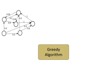
Kempe et al. (2003) present a greedy approximation algorithm applicable to IC and LT models. The algorithm requires computing marginal gain of influence spread of every node v, σM(S ∪ {v}) - σM(S), in each iteration. The node with highest marginal gain is 'greedily' added to the seed set until the size of the seed set reaches k. We will discuss the greedy algorithm further in Chapter 2 of this thesis.
The greedy algorithm for influence maximization requires 2 inputs (figure 9) as follows (Goyal et al. 2011):
a) A social directed network graph G(V,E) and b) Influence Probability of each edge in E.
Greedy
Algorithm
Influential Nodes Social Network Graph G with influence
probabilities
Figure 9: Greedy algorithm requires Social network graph with influence probabilities.
spread of each and every nodes which can be quite time consuming if the number of nodes and edges in the social network graph is very large. Most of the work, such as work of Leskovec et al. (2007) and Chen et al. (2009, 2010), that followed in the area of influence maximization attempt to tackle the efficiency issue of the greedy approach. We discuss some these works in Chapter 2 of the thesis. However, this is to be noted that tackling scalability is not within scope of this research and we keep the discussion on this issue limited.
Another major issue that is largely ignored in the works in influence maximization, such as (Kempe et al. 2003) and (Chen et al. 2010), is the question – How and where we can compute Influence Probability? Here, it is assumed that the network itself and influence probabilities are known and given to the algorithm as input. A social network graph G can be easily constructed if the data is explicitly available (Goyal et al 2011). However influence probabilities are not explicitly available. In most of the literature reviewed, influence probabilities are assumed to be given as input (Bonchi et al. 2011). To conduct experimentation researchers adopted various trivial methods of assigning influence probabilities (Bonchi et al. 2011). For example assuming uniform link probabilities (e.g. all link have probability p = 0.01), or the trivalency (TV) model where link probabilities are selected uniformly at random from the set {0.1, 0.01, 0.001}, or assuming the weighted cascade (WC) model, that is p(u, v) = 1/dv where dv represent the in-degree of v (Goyal et al. 2011).
Goyal et al. (2011) recently compared these above methods and compared the different outcomes of the greedy algorithm. The finding of their experiments shows that the seed sets extracted under different probabilities settings are very different (with empty or very small intersection). This shows the importance of computing influence probability from real data instead of assigning them based on some naïve assumptions (Goyal et al. 2011). To tackle this issue researchers are now looking into ways to mine influence probabilities from Action Log of users in a social network (Goyal et al. 2010). Action log is a relation Actions(User, Action, Time) which contains tuples, for example (u, a, t), which indicates that user u (such that u∈V) performed action a, at time t (Figure 10b).
investigated. Finally, the authors also show that using the proposed method they can also predict whether a user will perform an action and when with high accuracy. We discuss this method further in Chapter 2 of this thesis.
u1 u5
u2
u4
u3
Figure 10: a) Social Network Graph. b) Action Log
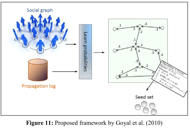
Goyal et al. (2010) propose to apply their method as a preprocessing step of influence maximization algorithms, such as Greedy by Kempe et al. (2003) or CELF by Leskovec et al. (2007). The overall framework of this method can be demonstrated by figure 11. In this framework Goyal et al. (2010) suggests to first learn influence probabilities from social graph and propagation log (or Action Log) and then apply Greedy (Kempe et al. 2003) or Lazy optimization (Leskovec et al. 2007b) algorithm to discover the seed set. We discuss these methods further in Chapter 2 of the thesis report.
Figure 11: Proposed framework by Goyal et al. (2010) (Bonchi et al. 2011. Pg. 11)
Therefore in this research our goal, though same as the works discussed above (i.e. discovering influential nodes), but different in the sense that we consider both positive and negative influence among users in a trust network to discover influential nodes. In the following section we summarize the problem definition and outline the contributions of the proposed research.
1.7 Thesis Contribution
consider trust social network where relationship is either trust or distrust. Such relationships in trust networks are asymmetric, meaning an existence of an edge (u,v) does not necessarily mean existence of an edge (v,u) (Guha et al. 2004). For example in a trust network, as defined in section 1.3, a positive edge (u,v) signifies that node u trust node v, but not vice versa. There are several examples of trust network in online domain For example, users on Wikipedia (www.wikipedia.com) can vote for or against the nomination of others to adminship; users on Epinions (www.epinions.com) can express trust or distrust of others; and users on Slashdot (www.slashdot.com) can declare others to be either “friends” or “foes” (Leskovec et al. 2010). Existing diffusion models for IM are modeled such a way that a node’s probability of performing an action (or adopting a product) will increase as the number of his/her friends performing the same action increases. However, we argue that, a node’s probability of performing an action (e.g. Buy iPhobe 4S) should also decrease if its distrusted users, also buy iPhone 4S.
Motivated by this the formal problem definition we propose to tackle is as follows:
Thesis Problem Definition – Find Influential Nodes from a directed trust network graph, G(V,E) with every edge (u,v) of E is directed and labelled either positive (trust) or negative (distrust), and Action Log, Actions(User, Action, Time) such that every user u in User column of action log table is member of V.
To solve the above problem we make the following contribution in this research:
1) We propose a new diffusion model named Trust-General Threshold (TGT) model which incorporates both positive and negative influence probabilities based on trust relationship among users in trust network.
2) Based on this new TGT model we propose a new influence maximization framework for trust network, called Trust-Influential Node Miner (T-IM), which takes trust network data and action log to find influential nodes.
trusted and distrusted users and use it to compute both positive and negative influence probability using Bernoulli distribution.
3) We show that approximation guarantee of (1-1/e) by existing IM algorithms such as Lazy Forward by Leskovec et al. (2007) is not applicable to TGT model because the influence spread function in this model is non monotonous.
4) We also show that influence spread function is still sub modular and define the problem of finding influential nodes from trust network under TGT model as an optimization of non-monotone submodular function problem.
4) We propose a new algorithm, mineSeedLS, based on local search (Lee et al. 2009) to solve IM under our proposed TGT model.
CHAPTER 2
RELATED WORKS
Analyzing information diffusion and social influence in social network has many applications to real-world. Influence maximization for viral marketing is an example of such an important application (Tang et al. 2009). In this section, we introduce the problem of influence maximization and review recent research progress. In section 2.1 we introduce some vocabulary related to information diffusion (Gruhl et al. 2004) process and also discuss several diffusion models that attempts to describe the diffusion process in social network. Most works, such as (Kempe et al. 2003, Leskovec et al. 2007b, Chen et al. 2010) on influence maximization problem rely on these models. In section 2.2 we discuss the classical paper by Kempe et al. (2003), where they first formulated the influence maximization as a discrete optimization problem and solved it using a greedy algorithm. In section 2.3 we discuss ‘Lazy forward’ optimization, by Leskovec et al. (2007), which is about 700 times faster than greedy of Kempe et al. (2003). In section 2.4 we discuss further improvement to the greedy approach mainly in terms of scalability. In section 2.5 we discuss some of the more recent data mining based approaches, such as by Goyal et al. (2010) in this area.
2.1 Diffusion Models
A diffusion model, also known as propagation model, describes the whole diffusion process and determines how the influence propagates through the network. The role of these diffusion model is primarily, to replicate or simulate real life diffusion process and determines which nodes and how many nodes will be activated by any given set of nodes (called seed nodes) after the diffusion process is over. There are few classical models which are used very commonly used to tackle the influence maximization problem. Here, we review some of them.
The status of the chosen set of users to market (also referred to as “seed nodes”) is viewed as active and initially all other users are considered inactive. Then, the chosen activated users, may further influence their friends (neighbour nodes) to be active as well. In this section we discuss the two of the most well known models namely Linear Threshold Model (LT) and Independent Cascade Model (IC) (Kempe et al. 2003). These models, or their variations, are most commonly used diffusion models in Influence Maximization.
2.1.1 Linear Threshold Model
Given a directed graph of social network G(V,E). A threshold value 𝜃𝑣 is assigned to each node v in V. Also each edge (u,v) in E is also assigned with a weight value bu,v. In linear threshold model the probability of a vertex v to become active will increase as more of its neighbours become active. The vertex v is influenced by each of its neighbour w according to the weight bw,v such that sum of all the weights bw,v for all w∈ Nv is ≤ 1. Where Nv is set of all active neighbours of v. At any given time t a vertex become active if
� 𝑏𝑤,𝑣 ≥ 𝜃𝑣 𝑤∈𝑁𝑎(𝑣)
The LT Model can be summarized using the following steps:
Given
- Threshold 𝜃𝑣
- Seed Sets A ⊆ V In time t
• Vertices that are active at time t-1 will remain
active
• Inactive vertex v becomes active at time t+1 if
� 𝑏𝑤,𝑣 ≥ 𝜃𝑣 𝑤∈𝑁𝑎(𝑣)
•
STOP when no nodes becomes activeExample:
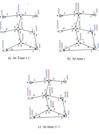
Let us now look at an example of an LT model. Let us consider the social network graph at time t-1 as shown in figure 12.a below. Let us also consider A = {a, c, i}, meaning nodes a, c and i are initially activated. The left column bar on each node represents the threshold 𝜃 and each directed edge has a weight value𝑏𝑤,𝑣. For example 𝑏𝑖,ℎ is .1 and 𝑏𝑎,𝑏 is .3.
At time t (Figure 12.b) node b be will be active as 𝑏𝑎,𝑏+𝑏𝑐,𝑏= 0.3 + 0.3 = 0.6 ≥ 𝜃𝑏. Similarly node f becomes active at time t as 𝑏𝑖,𝑓= 0.4 ≥ 𝜃𝑓. Note here that nodes g and h do not get activated here as the total weight of active neighbours (right column bar) is less than their respective threshold𝜃.
a)
At Time
t-1
b)
At time
t
c)
At time
t+1
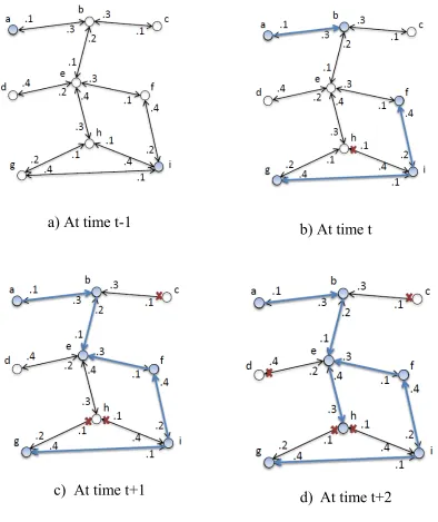
2.1.2 Independent Cascade Model
In independent cascade model every arc (u,v) in G(V,E) is associated with the influence probabilityp(u,v)of u influencing v. Influence Probabilities is the probability of a node to be influenced by another node. At time t, nodes that became active at t-1 will activate their inactive neighbours according to probability p(u,v). The IC Model can be summarized using the following steps:
Given
- Seed Sets A ⊆ V At time t
If u becomes active at time t-1
u attempts to activate each of its inactive neighbours v.
u activates v with probability p(u,v)
If successful, v becomes active in step t+1
STOP when no nodes becomes active
Example:
a) At time t-1
b) At time t
c)
At time t+1
d)
At time t+2
Figure 13 –
Independent Cascade Model example.
2.2 Greedy algorithm for Influence Maximization
the viral marketing problem, choosing a good initial set of nodes (customers) to target, as optimization problem in the context of these models.
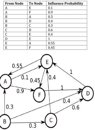
First they introduced diffusion models namely LT and IC (Section 2.1). Then they defined influence spread function, σ(.) as follows, given a network graph G(V,E) which is directed with influence probability or weight for each edge as shown in figure 14, and a diffusion model M, the influence of set of vertices A⊆ V, denoted σM(A) is the expected number of active vertices once the diffusion process is over. Using these notations we can formally define the k-best maximization problem as follows:
Problem 1(Influence Maximization) Given a social network graph G(V,E) along with influence probabilities of all edge in E, a diffusion model M and a number k find a set A⊆ V, |A| ≤k such that influence spread, that is σM(A), is maximum.
Kempe et al. (2003) prove that the optimization problem is NP-hard for both LT and IC Models. That is influence maximization problem as defined above cannot be solved in polynomial time. However they showed that σM(.) function is sub-modular and monotone.
Theorem 1(Kempe et al. 2003): For an arbitrary instance of the Independent Cascade Model or Linear Threshold Model, the resulting influence function is submodular and monotone.
According to Nemhauser et al. (1978) any submodular monotone function can be solved using natural greedy algorithm with a (1-1/e) approximation guarantee (Theorem 1).
Theorem 2(Nemhauser et al. 1979): The greedy algorithm gives a (1 – 1/e) approximation for the problem max{f (S) : |S| < k} where f is a monotone submodular function.
by initializing seed set S to Null (line 1). Vertex w which maximize the marginal gain
σM(S∪{w}) - σM (S)is added to S at each iteration (line 3), until the |S|=k.
Table 5: Sample social network data with Influence Probability
From Node To Node Influence Probability
A E 0.1
A F 0.9
B A 0.3
B D 0.4
B C 0.3
C D 0.6
C E 0.4
D E 1
E A 0.55
E F 0.45
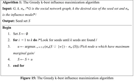
Algorithm 1: The Greedy k-best influence maximization algorithm
Input:G, k, σm /*G is the social network graph, k the desired size of the seed set and σm
is the influence model*/
Output: Seed set S
Begin
1. Set S← ∅
2. fori = 1 to kdo /*Look for seeds until k seeds are found /
3. u ← argmax w∊ V-S (σm(S ∪{w}) - σm(S));/Pick node u which have maximum
marginal gain/ 4. S ← S + u
5. endfor
Figure 15: The Greedy k-best influence maximization algorithm
For Step 3 of the greedy algorithm, the conventional method for estimating all the marginal influence gain of any node w in V, σm(S ∪{w}) - σm(S), with respect to current seed set S is described as follows (Kempe et al. 2003). First, a sufficiently large positive integer M is specified. For any node w ∈ V - S, the process of the diffusion model (IC or LT model) is run for the initial active set S and also for S∪{w}, and the number of final
active nodes activated by S (or S∪ {w}), denoted as ϕ(S) (or ϕ(S ∪ {w})) , is counted.
INPUT: A Seed Set S
OUTPUT: Average number of nodes activate by S (σ(S)) 1. For m = 1 to M do
2. Compute ϕ(S) /Compute # of users activated by S/
3. Set xm ← ϕ(S) 4. End For
5. Set σ(S) ← (1/M)∑𝑀𝑚=1𝑥𝑚 /Return the average # of users
activated by S/
Here, each ϕ(S) is computed as follows (Kimura et al. 2007):
1. Set H0 ← S ∪ {w}. /* H0 is set of currently active
users*/
2. Set t ← 0. /*Set time t to 0*/
3. while Ht is not ∅ do /*Until no new nodes are activated*/ 4. Set Ht+1 ← {the activated nodes at time t + 1}.
5. Set t ← t + 1.
6. end while
7. Set ϕ(S) ← ∑𝑡−1𝑗=0|𝐻𝑗| /Return total number of activated nodes by S/
Example:
To get this algorithm will compute the number of nodes activated by set S ∪ {w} for
each w ∈V \S under the independent cascade model. Following is the list of all nodes w ∈V\S and number of nodes that gets activated by each of these:
A – 4 as it activates nodes F, D and E B – 3 as it activates nodes D and E C – 3 as it activates nodes D and E D – 2 as it activates node E
E – 1 as it does not activate any more nodes F – 3 as it activates nodes D and E
Based on the above, the algorithm will choose node A in the first iteration and put it into set S. Now the seed set S = {A} and we still need to find one more node so that |S| = 2. In the second iteration the algorithm will compute marginal gain, σM(S∪ {w}) – σM (S) for each w ∈V\S, of each of the remaining nodes in V\{A}. Following is the list of nodes and its corresponding number of nodes activated by adding it to set S:
B – 2 as it activates node C
C – 1 as it does not activate any additional nodes.
D – 0 as it does not activate any additional nodes and D is already activated by set S E - 0 as it does not activate any additional nodes and E is already activated by set S F - 0 as it does not activate any additional nodes and F is already activated by set S
From the above numbers we can see that B has the highest marginal gain, i.e. activates most nodes. So node B is now added to set S which now has 2 nodes {A,B}. Since |S|=2 which was our required number of influential nodes the algorithm stops and here and return S={A,B}.
The resulting graph has 10748 nodes and 53000 edges. They compared their algorithm in three different models of influence – independent cascade model, the weight cascade model, and the linear threshold model. Also they further compared their greedy algorithm with heuristics based on node's degrees and centrality within the network, as well as choosing random nodes to target. The authors claim to have shown through experiments that their greedy algorithm significantly outperforms, in terms of influence spread, the degree and centrality-based heuristics in influence spread.
One of the main limitations of the above greedy approach is efficiency and scalability. Note that for selecting a node (step 3) that maximize the marginal gain σ(S ∪ {w}) - σ
(S) is computationally expensive, as it needs to explore all the possible combinations. Kempe et al. (2003) used Monte Carlo simulations, as discussed above, of the propagation model for sufficiently many times to obtain an accurate estimate (Goyal et al. 2011). As a result, finding a very small seed set in a relatively large network (e.g. 15000 vertices) could take days to complete in a modern server machine (Chen et al. 2009). Several recent studies aimed at addressing this efficiency and scalability issues such as by Leskovec et al (2007) and Chen et al. (2009, 2010).
2.3 ‘Lazy Forward’ Optimization
The most notable work in attempt to improve the scalability of greedy approach of influence maximization is by Leskovec et al. (2007). Leskovec et al. in (Leskovec et al. 2007b) tackle the problem of outbreak detection, which is the problem of selection of nodes in a network in order to detect the spreading of virus or information as quickly as possible. Though this work is not exactly in the area of influence maximization, the work done here contributed towards improving the scalability.
The authors refer to the work of Kempe et al. [2003], and suggest that this work generalizes the work on selecting nodes which maximize the influence in social network.
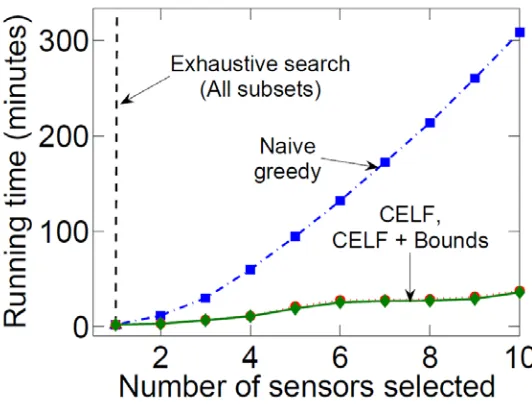
To take advantage of this property CELF algorithm maintains a table of marginal gain, mg(u,S), of each node u in current iteration sorted on mg(u,S) in decreasing order, where S is the current seed set and mg(u,S) is the marginal gain of u with respect to S. Table mg(u,S) is re-evaluated only for the top node in next iteration. If required the table is resorted. If a node remains at the top after this, it is picked and added to the seed set. Leskovec et al. (2007) evaluated their methodology extensively on two large scale real world scenarios namely: a) detection of contamination in large water distribution network, and b) selection of informative blogs in a network of more than 10 million posts. Using these scenarios they compared CELF's performance and scalability with natural greedy algorithm as shown in figure 16. In terms of performance, CELF generated results that are at most 5% - 15% from optimal. In terms of scalability, CELF also performed a lot better than greedy. For example for selecting 100 influential blogs, the greedy algorithm require 4.5h, while CELF takes 23 second (about 700 times faster). Also memory usage of CELF is about 50 MB compared to 3.5 GB required for greedy algorithm.
Example:
Let us consider the same example we discussed in the previous section. Consider the social network graph in figure 14 with given influence probabilities. Again let us set k=2, ie we are looking for the seed set of size 2. Similar to the greedy approach CELF optimization will pick node A in the first iteration and will also create a table mg(u,S) as follows:
Mg(A,{}) 4
Mg(B,{}) 3
Mg(C,{}) 3
Mg(D,{}) 2
Mg(E,{}) 1
As mentioned the algorithm will pick A as its marginal gain is the highest and will be removed from the table as follows:
Mg(B,{}) 3
Mg(C,{}) 3
Mg(D,{}) 2
Mg(E,{}) 1
2.4 Improving scalability of Greedy
2.4.1 MixedGreedy
Chen and Yang (2009) attempts to reduce run time of the greedy algorithm of Kempe et al. (2003) and its improvement by Leskovec et al. (2007). The authors point out that the work of Kempe et al. (2003) is not at all efficient. They claim that it would take days to find a small seed set in a moderately large network (e.g. 1500 vertices). Also though they acknowledge that the CELF algorithm by Leskovec et al. (2007) is 700 times faster, but they claim that it still takes few hours to complete in graph with few ten thousand nodes. Chen et al. (2009) tackle the efficiency issue of influence maximization by introducing new schemes to improve the greedy algorithm and combine it with CELF (named MixedGreedy) to obtain more efficient algorithm.
They conducted extensive experiments on two real life collaboration networks to compare their proposed approaches with CELF optimization. Experimental results showed that the for their new greedy algorithm the influence spread was exactly that of natural greedy algorithm of Kempe et al. [2003] and running time was 15-34% less than CELF.
2.4.2 CELF++
2.4.3 SimPath
Goyal et al. (2011b) attempt to design a scalable algorithm delivering high quality seeds for influence maximization problem under LT model. In Goyal et al. (2011) the authors highlighted several performance related drawbacks of simple greedy approach of Kempe et al. (2003) which are as follows: i) it requires to run Monte Carlo (MC) simulations sufficiently many times to estimate accurate influence spread which prove to be very expensive. ii) the greedy algorithm makes O(nk) calls to the MC simulations where n is the number of nodes in the graph and k is the number of seeds to be picked. They acknowledge the CELF optimization of Leskovec et al. improves the greedy, but stated that it still found to be quite slow and definitely not scalable.
To address these issues Goyal et al. propose the SIMPATH algorithm for influence maximization under the LT model. SIMPATH is built using CELF optimization that iteratively selects seeds in a lazy forward manner. SIMPATH make use of two key ways of optimizing the computation and improving the quality of seed selection which are as follows: i) Vertex Cover Optimization ii) Look Ahead Optimization.
For experiment they used four real-world datasets to evaluate SIMPATH and compare it with other well known influence maximization algorithms. The goal here was to evaluate in terms of efficiency, memory consumption and quality of the seed set.
The authors claim that qualities of seed sets, in terms of influence spread, generated by SIMPATH were quite competitive. For instance SIMPATH was only 0.7% lower than CELF in spread achieved and performed better compared to all other algorithms. In terms of efficiency, SIMPATH was fastest among all the algorithms; expect HIGH-DEGREE and PAGERANK of Page et al. (1998). Based on these results the authors claim that SIMPATH outperforms LDAG of Chen et al. (2010), in terms of running time, memory consumption and quality of seed sets.
2.4.4 Community-Based Greedy
computationally expensive and not suitable for a large mobile network. Also they mention that none of the previous works attempted to use community based approach for influence maximization. Wang et al. (2010) in their work proposes a new algorithm for mining top-K influential nodes, called Community-based Greedy algorithm (CGA). The idea behind their approach is to exploit the community structure property of social networks. CGA consists of two components 1) an algorithm for detecting communities based on information diffusion and 2) a dynamic algorithm to find influential nodes from these communities. To evaluate the effectiveness and efficiency of the proposed CGA algorithm the authors used data sets collected from call detail record (CDR) from China Mobile. They compared run time and influence spread of CGA with MixedGreedy of Chen et al. (2009), NewGreedy of Chen et al. (2009) and DegreeDiscount of Chen et al. (2010). The authors claim that the run time of CGA was faster than MixedGreedy but as expected was slower than heuristics based algorithms. However the experimental results showed that the influence spread of CGA was very close to MixedGreedy and NewGreedy. CGA outperformed the rest of the heuristic based algorithms quite comfortably. The authors claim that their approach is more than an order magnitude faster than the state of the art Greedy algorithm for finding top-K influential nodes.
2.4.5 Sparsification of Influence Network
In (Mathioudakis et al. 2011) the authors tackle the scalability issue of influence maximization problem by pruning the social network graph, called sparsification of network, while preserving the most of its properties. This work can be collocated with works on network simplification, the goal of which is to identify sub networks that preserve properties of a given network. They argue that such simplification of social network will yield significant improvement in terms of scalability. The authors define the problem of sparsification in terms of observed activity in the network. Given a social network and log of actions performed by nodes in the
that yields a finite likelihood. Then it greedily seeks a solution of maximum log-likelihood.
They used two real world data sets collected from Yahoo! Meme and a prominent online news site. To test their hypothesis that SPINE could play important role in reducing run time of influence maximization problem, they applied SPINE as preprocessing step to see if computation on sparsified network gives up any accuracy. For each network generated for collected datasets they measured the running time and influence spread before and after sparsification. Mathioudakis et al. (2011) claim that the experimental results shows that run time on sparsified network is considerably low compared to the full network. Also influence spread of seed set computed using sparsed network is quite close to that of the full network.
2.5 Data Mining Approaches
As highlighted earlier both greedy of Kempe et al. (2003) and its improvement, CELF by Leskovec et al. (2007) requires two kinds of data – a directed graph G, and assignment of probabilities or weights (depending on which diffusion model is considered) to the edges of G. A social network graph G can be easily constructed if the data is explicitly available. However influence probabilities or weights as used in LT and IC models are not explicitly available. In the work of Kempe et al. in (2003) and also the others listed above primarily made assumptions about these probabilities. The methods used to assign influence probabilities/weight to edges include the following (Bonchi et al. 2011):
i. Using constant value for all edges (e.g. 0.1)
ii. Choosing value uniformly at random from a small set of constant. E.g. {.1, .25, .5}
iii. Using nodes in-degree.