A first sketch: Construction of model defect priors inspired
by dynamic time warping
GeorgSchnabel1,∗and HenrikSjöstrand1
1Division of Applied Nuclear Physics, Uppsala University
Abstract.Model defects are known to cause biased nuclear data evaluations if they are not taken into account in the evaluation procedure. We suggest a method to construct prior distributions for model defects for reaction models using neighboring isotopes of56Fe as an example. A model defect is usually a
function of energy and describes the difference between the model prediction and the truth. Of course, neither the truth nor the model defect are accessible. A Gaussian process (GP) enables to define a probability distribution on possi-ble shapes of a model defect by referring to intuitively understandapossi-ble concepts such as smoothness and the expected magnitude of the defect. Standard specifi-cations of GPs impose a typical length-scale and amplitude valid for the whole energy range, which is often not justified, e.g., when the model covers both the resonance and statistical range. In this contribution, we show how a GP with energy-dependent length-scales and amplitudes can be constructed from avail-able experimental data. The proposed construction is inspired by a technique called dynamic time warping used, e.g., for speech recognition. We demonstrate the feasibility of the data-driven determination of model defects by inferring a model defect of the nuclear models code TALYS for (n,p) reactions of isotopes with charge number between 20 and 30. The newly introduced GP parametriza-tion besides its potential to improve evaluaparametriza-tions for reactor relevant isotopes, such as56Fe, may also help to better understand the performance of nuclear
models in the future.
1 Introduction
Evaluated nuclear data are important input for all kinds of nuclear physics applications. It has been shown in the past, e.g., [1], that evaluation techniques without proper account of potential model defects tend to underestimate uncertainties and bias results. Acknowledging the problem and being in need of a solution, Bayesian procedures have been often pragmati-cally tuned to deal with the problem, e.g., by ad-hoc adjustments of the likelihood function or by rescaling the obtained posterior uncertainties to make them plausible. A methodological elegant way is to introduce the information about model defects already as prior knowledge. In the field of nuclear data evaluation, this approach was pioneered by Pigni and Leeb [2]. Since then, various improvements and suggestions have been made, e.g., [3] and it was rec-ognized [4] that these developments essentially deal with the design of a covariance function for a Gaussian process (GP), e.g., [5]. GPs are flexible tools in the domain of non-parametric
Bayesian statistics but commonly used specifications, such as the squared exponential co-variance function, may not always be optimal for scenarios we encounter in nuclear data evaluation, e.g., quickly rising cross sections near thresholds or various degrees of predic-tive power of a nuclear model depending on the energy region where it is employed. So far this problem has been addressed by tailoring the covariance function to the specific situation, e.g., [6–8], whose shape can be adjusted by a few so-called hyperparameters.
Our suggestion in this paper is to replace the typically very structured covariance func-tion by a very flexible one and to infer its shape by taking into account reacfunc-tion systems that can be considered similar, i.e., the same reaction channels of neighboring isotopes. Formally, the amplitude and length-scale parameter—two numbers—of a standard squared exponen-tial covariance function are replaced by an amplitude function and a metric function. The introduction of the latter function was inspired by a technique called dynamic time warping used, e.g., in speech recognition [9] where the time axis is locally stretched and shrank to align different voice samples as good as possible. In our case, it is exactly the same idea: To modify the effective distance between energies in order to align the Gaussian process as good as possible to the experimental data of all reaction systems at the same time. We remark that a certain construction of a model defect based on the information of neighboring isotopes has already been suggested in [3]. A distinctive feature of our approach is the determination of the model defect by the maximization of a score function, i.e., the marginal likelihood.
This paper is structured as follows. In section 2 we introduce the new parametrization of a GP which we calldynamic time warping GPor DTW GP for short. In section 3 we derive the criterion to determine the amplitude function and metric function. In section 4 we demonstrate the feasibility of the data-driven approach to infer the model defect of TALYS for (n,p) reactions using data for 56Fe and neighboring isotopes. Finally, in section 5 we summarize and conclude.
2 DTW GP
The relation between experimental data and the model prediction can be written as
~σexp=M(~p)+~εdef+~εexp (1)
where~σexpcontains the experimental measurements,M(~p) is the corresponding model pre-diction based on the set of model parameters ~p, the vector ~εdef contains the deficiency of the model, and~εexp contains the errors of the measurements. The unobservable truth~σtrue is therefore given by bothM(~p)+~εdef and~σexp−~εexp. The only accessible quantity in this model is~σexp. The values in all other quantities are uncertain and we have to assign probabil-ity distributions to express our belief about the likelihood of possible realizations. Once all prior probability distributions are defined, we can use Bayesian statistics to obtain estimates of all quantities involved. In this section, we discuss the specification of a probability distri-bution for~εdef. The specifications of probability distributions for the other quantities follows in section 3.
For the following discussion, we assume that ~σexp in eq. (1) contains angle-integrated cross sectionsσexp,iof a single reaction channel measured at incident energiesEi. The
and the latter covariances between pairs of function values at arbitrary energies. Expressed in terms of our setting: For any choice of incident energiesE1,E2, ...the probability distribution of associated cross sections follows a multivariate normal distribution. We assume that the model prediction is a priori the most probable option, i.e.,µ(E)=0. A common choice for the covariance function is the so-called squared exponential form, e.g., [5], introduced in [4] for nuclear data evaluation,
k(E,E0)=δ2exp −1 2
(E−E0)2
λ2 !
. (2)
This form is a reasonable default but depending on the energy range and observable other forms may be more suitable. Some alternatives have been employed and studied in [6–8]. All of these alternatives, however, are still rather rigid in terms of their structure and therefore foremost good solutions for the observable and energy range for which they have been de-signed. In this paper, we aim to construct a very flexible covariance function that is capable to adapt to any setting. Therefore we suggest the covariance function
k(E,E0)=δ(E)δ(E0) exp −1 2
m(E)−m(E0)2 !
(3)
where both the amplitudeδand length-scaleλof the squared exponential form are replaced by an energy-dependent amplitude and metric function, respectively. We callm(.) a metric function because a distance (i.e. difference) between two energies gets transformed to another one. We demand the triangle inequality to hold, which is a defining criterion for a metric. Therefore, the functionm(.) must be monotonically increasing. The idea we pursue in this contribution is the determination of the functionsδ(.) andm(.) in a data-driven way by taking into account the same reaction channel of neighboring isotopes. The result for the (n,p) channel is displayed in fig. 2. The remainder of this and the next section deals with the parametrization ofδ(.) andm(.) and the method to infer its shape from the data.
We want a maximum of flexibility for the functionsδ(.) andm(.) and therefore suggest to define them as continuous piecewise linear functions. A continuous piecewise linear function can be written as
f(E| {zi}i=1..N)=
N−1 X
i=1
Ei+1−E Ei+1−Ei
zi+
E−Ei
Ei+1−Ei
zi+1
!
Ii(E). (4)
where the factorIi(E) =1 ifEi ≤ E <Ei+1 and zero otherwise. The defining parameters of this function are the function values{zi}i=1..N at energies{Ei}i=1..N, i.e., f(Ei) =zi. With
a dense enough energy grid, arbitrary functions can be well approximated. The flexibility of functions parametrized as in eq. (4) requires reasonable constraints on features of these functions, which can be regarded as prior knowledge. Plausible constraints can be formulated in terms of minimal and maximal allowed changes per energy unit. In order to properly formulate such constraints, we can make the variable transformation
zi(z0,∆z1,· · ·,∆zN)=z0+
i X
k=1
∆zk. (5)
Using this variable transformation, we obtain
With this definition, the piecewise linear functions parametrized in terms of differences of function values forδ(.) andm(.) can be written as
δ(E)=g(E|u0,· · ·,uN) andm(E)=g(E|v0, . . . , vN). (7)
In the next section, we discuss how to determine the parametersuiandviin a data-driven way
by optimization.
3 Marginal likelihood maximization
The determination of the parameters{ui}i=1..N and{vi}i=1..N in eq. (7) requires a score func-tion to assess the performance of possible solufunc-tions. In this secfunc-tion we derive one within the framework of Bayesian statistics. First, we have to complete the statistical model in eq. (1) by specifying the missing probability distributions for the model parameters~p, and the ex-perimental errors~εexp. We assume multivariate normal distributions for both of them, i.e.,
~εexp∼ N(~0,Kexp) andp~∼ N(~p0,Kpar). (8)
For the model defect we have~εdef ∼ N(~0,Kdef) with the elements of the covariance matrix Kdef determined by eq. (3). The assumption of a priori independence of ~p, ~εdef, and ~εexp completes the specification of the statistical model. In order to obtain analytic solutions, we further substitute the nuclear model by a first-order Taylor approximation
Mlin(~p)=~σmod+S(~p−~p0) (9)
with
~σmod=M(~p0) andS =
∂M(~p)
∂~p ~p=~p
0
. (10)
Now we can compute the evidence, i.e., the probability distribution associated with~σexp. This variable is multivariate normal because it is given as a sum of multivariate normal ran-dom variables. Therefore it suffices to calculate the associated mean vector and covariance matrix,
E[~σexp]=~σmod,
Var[~σexp]=M =S KparST+Kdef+Kexp,
(11)
to obtain the result that ~σexp ∼ N(~σmod,M) which corresponds to the probability density functionπ(~σexp), given for a specific realization~σ0expin eq. (12). Noteworthy, this distribution provides prior probabilities of possible outcomes of the experiment. As an aside, we remark that the underlying statistical computation—called marginalization—has been used for nu-clear data evaluation before [10]. Marginalization serves the purpose to get rid of variables not of interest by themselves but nevertheless to properly account for the extra uncertainty they introduce. Here we marginalized over nuclear model parameters.
adjusting the parameters{ui}i=0..Nand{vi}i=1..Nof eq. (7) which define the form of eq. (3) and
consequently alsoKdefto maximizeπ(~σ0exp),
logπ(~σ0exp)=−N
2 log(2π)− 1
2log|M| − 1 2χ
2, with (12)
χ2= ~σ0
exp−S~σmod T
M−1~σ0exp−S~σmod
. (13)
In other words, we seek to adjustδ(.) andm(.) of the covariance function to maximize the probability of the experimental measurements ~σ0exp. As a reminder, eq. (12) is the loga-rithmized multivariate normal pdf characterized by the mean vector and covariance matrix defined in eq. (11). Noteworthy, a linear transformation of the occurring vectors and cor-responding transformations ofS andMleave the value of the third term (i.e. theχ2term) invariant but alter the value of the second term containing the determinant. It seems more reasonable to us to penalize complexity on a relative scale and hence we used the transfor-mation ˜σi =(σi−σmod,i)/max(0.1, σmod,i) to transform~σexp and~σmodand also performed the corrsponding transformation on the sensitivity matrixS and the covariance matrixM. We expect the model to be less predictive for very low cross sections. To avoid unreasonable large uncertainty bands for such cross sections, we revert back to an absolute scale for cross sections below 0.1 millibarn, which explains the maximum in the denominator. The model defect is applied additively on this transformed scale. The amplitude functionδ(E) therefore roughly amounts to the relative deviation of the truth from the model if the underlying prior model cross section is greater than 0.1 mbarn.
We are interested to learn about theglobalpredictive power of the nuclear physics model. Thus we take reaction data of several neighboring isotopes into account for the maximization of eq. (12). We aim to find a set of{ui}i=0..N and{vi}i=0..Nthat is suited for a specific reaction channel, e.g., (n,p), for all the isotopes. Assuming experimental data and model parameters associated with different isotopes to be independent, we obtain the following form of the marginal likelihoodπ(~σ0exp):
logπ(~σ0exp)=−N
2 log(2π)− 1 2
Niso
X
i=1
log|Mi|+log Niso X
i=1
exp −1 2χ 2 i ! (14)
The sums run over the number of isotopesNisoand contain the covariance matrices Miand χ2values with respect to the individual isotopes.
4 Exemplary application
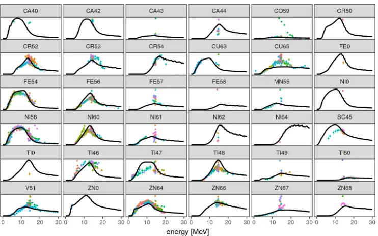
We determined the model defect covariance function by the outlined approach for (n,p) re-actions in combination with the nuclear models code TALYS [11]. Because we want to use the model defects for an evaluation of56Fe, we included angle-integrated cross section data for isotopes with charge numbers between 20 and 30 and incident energies between 0.1 and 30 MeV available in the EXFOR database [12]. We assigned an uncorrelated uncertainty of 10% to all the data points, which is sufficient for the purpose of demonstrating the outlined approach. The included experimental data for (n,p) reactions is displayed in fig. 1. As can be seen in the figure, we did not attempt to remove experimental outliers. Unfortunately, given space restrictions, we are not able to give proper credit to the authors of these measurements due the fact that the data is spread over 207 entries in the database. References to the data can be provided upon request.
Figure 1.Experimental data for angle-integrated (n,p) cross sections of isotopes with charge numbers between 20 and 30 used for the marginal likelihood maximization. Uncertainties of experiments are assumed to be 10% and independent across data points. An energy of zero corresponds to the threshold energy of the reaction. The mass number zero indicates natural composition. No efforts have been made to identify outliers or assess the quality of the data sets. The data were retrieved from 207 entries of the EXFOR database.
Figure 2.The dynamic time warping GP specification resulting from the marginal likelihood maximiza-tion: (left) the amplitude functionδ(.); (middle) the metric functionm(.); and (right) the corresponding model defect correlation matrix. Different curves in the left and middle figure correspond to different local maxima of the marginal likelihood. The majority of the ten optimization results coincide and in-dicate the global maximum. Due to the transformation of the cross sections described in the paragraph below eq. (12), the functionδ(E) can be interpreted as relative model defect expected a priori.
corresponds roughly to an energy resolution of 0.3 MeV and gives rise to 200 hyperparam-eters (i.e. theui’s andvi’s in eq. (7)) that have to be optimized. Importantly, we shifted the
origin of the energy grid to the threshold of the reactions. This measure ensures that cross sec-tions near thresholds of different isotopes are mapped to the same grid points of the Gaussian process and also peaks are potentially better aligned.
amplitude function may not change more than about three percent between consecutive grid points. In other words, we constrained the rate of change of the amplitude function to be below roughly 10% per MeV. As the metric function has to be monotonically increasing, we applied a lower limit of 0.03 and an upper limit of 0.15 for its change between consecutive grid points. This specification translates to the prior knowledge that the effective length-scale should be at least roughly 1 MeV and not larger than 10 MeV at any energy. The lower limit on the effective length-scale protects against discrepant data, which would elsewise drive the effective length-scale to unreasonable low values. We emphasize here again that the dy-namic amplitude and length-scale determined in a data-driven way is the real novelty of our approach. We derived analytic expressions for the gradient of the marginal likelihood, see, e.g., [14], which can be exploited by the L-BFGS-B algorithm. We performed the optimiza-tion ten times with different starting values and achieved in all cases convergence. Averaged over the individual optimization runs, it took the algorithm about 630 iterations to converge— tens of minutes on a decent personal computer with eight cores. Even though there were two local maxima, the majority of calculations converged to the global one. The learned am-plitude and metric function as well as the correlation matrix of the model defect are shown in fig. 2.
5 Summary and conclusion
We introduced a new parametrization of the covariance function based on the concept of an amplitude and metric function and showed how these functions can be inferred from exper-imental data for neighboring isotopes by maximizing the marginal likelihood. We demon-strated the feasibility of the approach with the nuclear models code TALYS [11] and (n,p) reaction data for isotopes with charge numbers between 20 and 30. The obtained amplitude function and metric functions are interesting by themselves because they potentially allow us to gain not only qualitative but also quantitative insight into model performance on a per-energy basis. In the future, these model defects constructed by taking a global view on the predictive performance of nuclear models can be included in evaluation procedures to obtain more robust and reliable results.
References
[1] P. Helgesson, D. Neudecker, H. Sjostrand, M. Grosskopf, D.L. Smith, R. Capote, As-sessment of Novel Techniques for Nuclear Data Evaluation, inASTM 16th International Symposium on Reactor Dosimetry(Santa Fe, New Mexico, 2017)
[2] M.T. Pigni, H. Leeb,Uncertainty Estimates of Evaluated56Fe Cross Sections Based on
Extensive Modelling at Energies Beyond 20 MeV, inProc. Int. Workshop on Nuclear Data for the Transmutation of Nuclear Waste. GSI-Darmstadt, Germany(2003) [3] H. Leeb, D. Neudecker, T. Srdinko, Nuclear Data Sheets109, 2762 (2008) [4] G. Schnabel, Ph.D. thesis, Technische Universität Wien, Vienna (2015)
[5] C.E. Rasmussen, C.K.I. Williams, Gaussian Processes for Machine Learning (MIT Press, Cambridge, Mass., 2006), ISBN 0-262-18253-X 978-0-262-18253-9
[6] G. Schnabel, H. Leeb, EPJ Web of Conferences111, 09001 (2016) [7] G. Schnabel, arXiv eprint arXiv:1803.00928 (2018)
[8] P. Helgesson, H. Sjöstrand, Review of Scientific Instruments88, 115114 (2017) [9] C. Myers, L. Rabiner, A. Rosenberg, IEEE Transactions on Acoustics, Speech, and
[10] Cyrille De Saint Jean, G. Noguere, B. Habert, B. Iooss, Nuclear Science & Engineering
161, 363 (2009)
[11] A.J. Koning, S. Hilaire, S. Goriely, TALYS-1.6 - A Nuclear Reaction Program, http://www.talys.eu (2013)
[12] N. Otuka, E. Dupont, V. Semkova, B. Pritychenko, A. Blokhin, M. Aikawa, S. Babyk-ina, M. Bossant, G. Chen, S. Dunaeva et al., Nuclear Data Sheets120, 272 (2014) [13] R.H. Byrd, P. Lu, J. Nocedal, C. Zhu, SIAM Journal on Scientific Computing16, 1190
(1995)