Critical Issues in Modelling Lymph Node Physiology
Dmitry Grebennikov1,2, Raoul van Loon3, Mario Novkovic4, Lucas Onder4, Rostislav Savinkov2,5, Igor Sazonov3, Rufina Tretyakova2,5, Daniel J. Watson3and Gennady Bocharov2,*
1 Moscow Institute of Physics and Technology (State University), Dolgoprudny, Moscow Region 141701, Russia; [email protected]
2 Institute of Numerical Mathematics of the RAS, Moscow 119333, Russia; [email protected] (R.S.); [email protected] (R.T.)
3 College of Engineering, Swansea University, Swansea SA2 8PP, Wales, UK; [email protected] (R.v.L.); [email protected] (I.S.); [email protected] (D.J.W.)
4 Institute of Immunobiology, Kantonsspital St. Gallen, St. Gallen 9007, Switzerland; [email protected] (M.V.); [email protected] (L.O.)
5 Lomonosov Moscow State University, Moscow 119991, Russia * Correspondence: [email protected]; Tel.: +7-905-554-4383
Abstract:In this study we discuss critical issues in modelling the structure and function of lymph nodes (LNs), with emphasis on how LN physiology is related to its multi-scale structural organization. In addition to macroscopic domains such as B-cell follicles and the T cell zone, there are vascular networks which play a key role in the delivery of information to the inner parts of the LN, i.e., the conduit and blood microvascular networks. We propose object-oriented computational algorithms to model the 3D geometry of the fibroblastic reticular cell (FRC) network and the microvasculature. Assuming that a conduit cylinder is densely packed with collagen fibers, the computational flow study predicted that the diffusion should be a dominating process in mass transport than convective flow. The geometry models are used to analyze the lymph flow properties through the conduit network in unperturbed-and damaged states of the LN. The analysis predicts that elimination of up to 60−90 % of edges is required to stop the lymph flux. This result suggests a high degree of functional robustness of the network.
Keywords: computational model; lymph node; multiscale structure; vascular network; fibroblastic reticular cells; conduit network; lymph flow; destruction of conduits
1. Introduction
The immune system functions to protect the host against various pathogens and tumours. The mammalian immune system is a complex compartmentalized population of different types of humoral factors and cells organized as a body-wide network of interacting lymphoid organs, e.g., bone marrow, thymus, spleen, lymph nodes, gut. Its elements are connected by two vascular systems, i.e., the blood and the lymphatic systems, that enable the immune elements to migrate continuously to or from the compartments during their lifetime. Lymph nodes (LNs) represent the most numerous compartments of the immune system, in which soluble signals and cells are concentrated to enable efficient interaction between them. The structure of a LN is crucial to its function [1]. The development of anatomically correct mathematical models that accurately reproduce the physiological, cellular and molecular processes in LNs remain one of the major challenges for mathematical immunology.
regions. The multi-physics description of the lymph flow processes combines the conservation of mass and momentum equations in subcapsular and medullary sinuses (fluidic region) with the conservation of mass and Darcy’s law with Brinkman’s term for the flow in porous regions. This study can be considered as a milestone for the application of computational fluid dynamics and the whole-organ fluorescent imaging technologies to model the LN physiology.
Lymph nodes are characterized by a highly variable histological appearance. This implies that the development of computational models of the LN structure and function requires(i)an idealization of the structure,(ii)the implementation of a modular approach, and(iii)the analysis of the performance of specific functional LN units in health and disease. The elements of the above framework can be found in [3–7].
LNs are known to present high resistance to lymph flow [3], which results from the internal structure of the LN body comprised of blood microvascular networks, the conduit networks and of domains densely packed with immune cells, i.e., the B cell follicles and T cell zone. In the existing 3D geometry LN models developed for studying the fluid flow, the conduit and blood vascular systems are not structurally described. Meantime, these elements, in particular the conduit system network ensheathed by fibroblastic reticular cell (reticular) network, represent a key system for the delivery of soluble molecules in the paracortex area of the LN. It was estimated in [3] that under normal conditions about 10 % of lymph entering the LN through the afferent vessels takes a central path to reach the efferent vessel and high endothelial venules (HEV) via the conduit system and the inner domain of the LN. Under inflammatory conditions and during infections, the conductivity of the conduit system is likely to change dramatically [8], which affects the information delivery (cytokines, hormones, etc.) to the reactive parts of the LN. A fine and elaborate structure of the LN vascular systems requires the development of multi-scale computational models to comprehensively examine the fluid transport in LNs.
In this study we present an overview of the critical issues in modelling the structure and function of LNs and propose some approaches to model the networks of fibroblastic reticular cells, the blood microvasculature and analyze the flow properties of lymph through the conduit network in an unperturbed state and a damaged state with the varying degrees of destruction. We review the major structural elements of LNs in Section 2. The approaches to model the geometry of an a FRC network and the blood microvascular network are presented in Section 3. A fine resolution analysis of the lymph transport through a single conduit are presented in Section 4. The hydraulic conductivity properties of normal and disrupted conduit systems, modelled as 1D topologically equivalent networks are studied in Section 5. Numerical assessment of the percolation robustness of the fibroblastic reticular cell (FRC) network is predicted in Section 6. Further perspectives for application of computational fluid dynamics techniques are discussed in Section 7.
2. Major Structural Elements of a Paradigmatic Lymph Node
[12–14]. Furthermore, FRCs support lymphocyte migration, retention and survival through expression of chemokines CCL19 and CCL21 [15] and survival factor IL-7 [16,17]. FRCs secrete a basement membrane enwrapping the inner core of LN conduits which consist of collagen fibers and extracellular matrix (ECM) components. The conduit system drains lymph from the SCS through the entire LN T cell zone and the interstitial lymph flow accommodates small molecules and antigen that are<80 kDa in size. Some DCs are capable of extending their cell protrusions into the conduits, enabling them to sample the inner core for foreign antigens [18]. Apart from the lymphatic system in LNs, a specialized blood vascular system permeates through the LN T cell zone, forming high endothelial venules (HEVs) [8,19] which serve as extravasation points for migrating T, B cells and DCs into the LN [20]. Despite technical limitations in terms of rendering difficulties in the assessment of structural information from whole LNs, recent advances in imaging and computational techniques have enabled a comprehensive quantification of e.g. the LN blood vascular network [8,21].
The complexity of the immune system has been recognized in the recent decade as one of its key hallmarks, but also a major challenge for integrative immunological research [22]. Nevertheless, the development of high throughput “-omics” methods [23] and systems biology approaches [24] has made it possible to dissect the spatiotemporal interactions between immune system constituents and reveal functional implications in the context of various diseases. In order to fully utilize systems approaches, it is necessary to integrate available data across multiple biological scales, from lower level processes such as gene expression in different cell populations to higher level processes such as maintenance and regulation of tissue and organ functionality [25]. Finally, the complex dynamics of the immune system can be elaborated from the content-rich observations of these processes.
Increasing computer processing capabilities has made it feasible to design and generate a paradigmatic LN model based on real organ geometry [4]. Such a systems biology approach has allowed us to develop a generalized 3D solid model of the LN, which consists of the following idealized structures: SCS, B cell follicles, trabecular and medullar lymphatic sinuses, blood vasculature and HEVs, the T cell zone and FRC network. An integrated LN model across multiple scales will allow detailed description of global spatiotemporal dynamics of the different cell type interactions and enable us to identify biological parameters that are critical for generation and maintenance of immune responses.
3. Computational Models of FRC- and Blood Vascular Networks of Lymph Nodes
3.1. Cellular Potts Modelling of the FRC network
In this section we construct a geometrical model of reticular network using the Cellular Potts Model (CPM). This approach lets us explicitly control the target volume of reticular network, vary properties of each FRC, and directly incorporate the network in further models of cellular immune response. In addition, it is a starting point of modelling reticular network as soft tissue, which would let us explore mechanical properties and behavior of the network in cases of inflammation, T cells depletion or LN fibrosis.
In CPM (reviewed in [26–29]), the cells are defined on a cubic lattice as connected collections of lattice cites (voxels)v ={i,j,k}with the same cell idσ(v). Each cell can belong to a certain typeτ(σ(v)). The extracellular medium is defined as a generalized cell withσ=τ=0.
The energy of the system is usually defined as the sum of two terms:
E=Eadhesion+Evolume=
∑
neighborsv1,v2:
σ(v1)6=σ(v2)
J(τ(σ(v1)),τ(σ(v2))) +
∑
σ
λ(σ) V(σ)−Vtarget(σ)2 (1)
Adhesion term represents the sum of binding energies J(τ(σ(v1)),τ(σ(v2))) of molecules located at
adjacent pairs of voxelsv1,v2, which correspond to membranes of different cellsσ(v1),σ(v2). The second
term describes the ability of the cell to constrain its volumeV(σ)near the resting volumeVtarget(σ)due to the internal pressure. The parameterλ(σ)is a spring modulus, i.e. the rigidity of the cell to changes of volume. It determines the relative weight of the second energetic term. There are many other possible terms and modifications of the form of energy,E, which allow the modelling of compressibility of cells membranes, chemotaxis, haptotaxis, cell elongation and other processes [26,27,29,31].
The basic form of the probability acceptance function in CPM is given as,
p(σ(vsource)→σ(vtarget)) =min
1, exp
−∆E
T
, (2)
where T is a global parameter representing the amplitude of cells fluctuations, proportional to the probability to accept energetically unfavourable voxel-copy attempts,∆E=Ea f ter−Ebe f oreis the change
of energy of the system (1) as a result of sampled voxel-copy attempt. IfT = 0, the simulation is fully determinate and can freeze at local energy minima. As a possible extension of (2), each cell type or each cell can have its ownT(σ).
The other form of acceptance function, which provides a biologically relevant meaning of parameter T(σ)— the intrinsic motility of the cell (discussed in detail in [29]), was specified as follows,
p(σ(vsource)→σ(vtarget)) =tanh(Tm)·min
1, exp
−∆E
Tm
, (3)
where
Tm=
(
T(σ(vsource)), i f σ(vsource)6=0
T(σ(vtarget)), i f σ(vsource) =0
is the resultant motility of membrane between σ(vsource) 6= σ(vtarget). Given the tanh-mapping of
membrane motility, function (3) restricts the voxel-copy attempts involving so-called frozen cells (with T(σ) →0), even if calculated∆Eis significantly negative. This allows us to specify the motility of cells, i.e. their ability to react on external stimuli.
We extend this approach by setting intrinsic motility for each voxel of the cell. By doing this, we can easily model the reticular network, making the ends of protrusions frozen (forming FRC junctional complexes [30]). As a result, there is no need for extra assumptions and extra CPM plugins such as cell elongation or connectivity constraints (which are computationally expensive in 3D [31]), utilized in other models of cellular networks (such as in the study of vasculogenesis [31]).
We initialize cells as thin (d ∼ 1.0µm) cylinders along the graph of reticular network topology (constructed in [4]), forming the conduit system (Figure1a). Protrusions of different cells are connected at the middles of the corresponding edges. For each FRC we define the center of it’s bodyvc(σ)at the coordinates of corresponding graph nodes. We define the motility of voxels occupied with cells (v(σ)) according to the distribution localized aroundvc(σ):
T(v(σ)) =Tmax·exp
− kv(σ)−vc(σ)k2 .
By doing this, the voxels, which are far from the center of FRC bodyvc(σ), have close to zero motility T(v(σ)) → 0. As a result, the ends of FRCs protrusions are linked with each other in accordance with given topology and are not altered during the simulation, resulting in no connectivity issues. The voxels which are closer to centersvc(σ)have more intrinsic motility, thus it is more probable for them to extend to the medium due to internal pressure until the FRCs would reach their target volumeVtarget(σ).
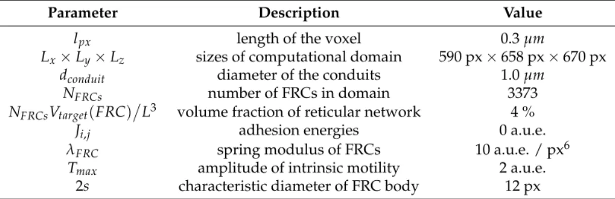
Figure1b illustrates the reticular network, reached it’s target volume (4% of the whole volume of lattice [4]). It contains 3373 FRCs in a 177.0µm×197.4µm×201.0µmcomputational domain withlpx=
0.3µmlength of the voxel resolution. Parameters used in the simulation are listed in Table 1. We set adhesion energies to zero because they are not relevant for the result as there are no other cells in our model. The choice of FRC-FRC adhesion energy doesn’t affect the simulation because FRC junctional complexes are modeled by freezing the ends of protrusions. A high value for lamda is chosen (λ(σ)1) because of rigidity of the reticular networks. The deviation of volume from the target volume for the whole network is less than 1% after 20 Monte-Carlo steps (MCSs) burn-in period.
(a) (b)
Figure 1. (a) The initialized reticular network as the system of conduits of given topology. State of the simulation at MCS=0. (b) The reticular network reached its target volume. State of the simulation at MCS=20.
Table 1. Parameters of Cellular Potts Model used to generate the reticular network (a.u.e. stands for arbitrary units of energy).
Parameter Description Value
lpx length of the voxel 0.3µm
Lx×Ly×Lz sizes of computational domain 590 px×658 px×670 px
dconduit diameter of the conduits 1.0µm
NFRCs number of FRCs in domain 3373
NFRCsVtarget(FRC)L3 volume fraction of reticular network 4 %
Ji,j adhesion energies 0 a.u.e.
λFRC spring modulus of FRCs 10 a.u.e. / px6
Tmax amplitude of intrinsic motility 2 a.u.e.
The implementation of the model is based on the open-source CompuCell3D application (available at http://compucell3d.org/). We modified the source code of its core C++ library to accomplish voxel-based motility and developed Python scripts to configure the simulation. The computation of the FRC network shown in Figure1requires about 10 min real time on Intel Xeon 4-core 3 GHz CPU with 4 Threads based parallelization.
3.2. Modelling Blood Vascular Network
The vascular network of a lymph node is a rather complex construct and is placed inside the internal space of the LN with various items, such as B-cell follicles, FRC network, medullar and trabecular zones. The vascular network provides the delivery of oxygen, nutrients and signal molecules. Lymphatic fluid can leave the LN through the blood vessels due to a pressure difference, hydrostatic and osmotic, between the interstitial pressure in the node and the pressure in the blood vessels [2,3]. The vessels of the blood microvascular network have lots of close intersections with the FRC network, pervading the whole space inside LN, so the vascular network influencesshma many processes in the lymph node. In this way, construction of a 3D model of vascular network provides an insight into the role of the vascular network in processes of tissue homeostasis and pathology.
While constructing the vascular network, we had to solve some problems with intersections of the FRC network, vascular network and internal items of the an LN. The main challenge there was to overcome the differences between the typical sizes of the networks. An FRC network consists of conduits with a diameter range from 0.2 to 2 µm, while the vascular network contains vessels with a diameter range from 5 to 30µm [21]. We modified the algorithm from [7] to meet these conditions.
3.2.1. Initial Data
We used data from [21] to set the length of the network vessels. The blood microvascular system
0 20 40 60 80 100 120 140 160 180 200
Vessels length, µm
0 200 400 600 800 1000 1200
Relative number
Figure 2.Blood vessels length distribution summarized from [21]
is characterized by the length of vessels and branch separation from the feeding vessel. The number of capillary vessels was taken from [21] as 40 vessels. It could be approximated as 3 vessels with 5 bifurcations (32 vessels) and 1 vessel with 6 bifurcations (64 vessels), the diameter of input and output vessels was taken as 8µm.
3.3. Algorithm of Network Graph Generation
Step 1. Graph topology organisation. In this step we generate the basis points and edges of connections. Step 2. Local edge length optimization. In this step we use the algorithm from [7] just for a local (i.e., for
neighbouring nodes) adjustment of the mismatch of the model and target graph edges lengths . In this and the next steps, the following parameter from Step 1 is used: blos(defined on line 4 in the pseudocode). It’s the canonical length of segments of the vessels graph.
Step 3. Global network structure optimization. In this step we use a modified algorithm from [7] for
(i) minimization of the edge length deviation from the real data for all neighbouring nodes, (ii)
pushing apart disconnected nodes from each other to prevent merger of the vessels, and (iii)
shifting the nodes away from the prohibited domains associated with other LN structures.
Pseudocode of Step 1 (graph topology organisation): // Initialise the data arrays
1set”length distribution”as real arrayld; 2set{5 5 5 6}as integer arraybf;
// Specify the segmentation accuracy, vessels radius and decreasing, processing zone size 3set”initial input/output vessels diameter”as realvd;
4set4.0as realblos; // length of segmentation of the vessels,µm 5set212 as realrf; // coefficient of vessels radius decreasing
6set”work sphere radius”asR; // simplify the constructing 7set graph structuret;
// Attach the input and output vessels
8insert line”input vessel”and line”output vessel”tot; // simple lines, splitted into 100 segments 9 f or(integerj=1to NC)begin
// In this loop, we create new vessels, growing frominputandoutputvessels 10 set realvdl = vd;
11 set realsl = random f romld; 12 sl = sl/blos;
13 set integersc = sl; 14 sl = sl − sc;
15 i fsl > 0.5thensc = sc + 1;
//scdefines the number of segments for current generating line 16 set pointpin = random point f rom input vessel;
17 set pointpout = random point f rom output vessel;
18 set pointpm11 = random point f rom sphere with radius R; 19 set pointpm12 = random point f rom sphere with radius R; 20 set pointpm21 = random point f rom sphere with radius R; 21 set pointpm22 = random point f rom sphere with radius R;
// we used pointspmXXto avoid helical structures while the second and // third parts of graph construction.
22 init linelx1that goes f rompintopm12throughpm11splitted intoscsegments; 23 assignvdlaslx1diameter;
24 insert linelx1tot;
25 init linelx2that goes f rompouttopm22throughpm21splitted intoscsegments; 26 assignvdlaslx2diameter;
27 insert linelx2tot;
30 f or(integeri=1tonbf)begin
// In this cycle in each loop we create two sub-vessels for each // couple [lx1,lx2], created while previous loop
31 set realvdl = vd rfi;
32 setpm12 f romlx1as pointpin; 33 setpm22 f romlx2as pointpout;
34 i f(i < nbf)then execute code lines f rom11to15, f rom18to26; 35 i f(i = nbf)then begin
// here we connect the inner and outer parts of vessel 36 execute code lines f rom11to15;
37 set pointpm1 = random point f rom sphere with radius R; 38 set pointpm2 = random point f rom sphere with radius R; 39 set pointpm3 = random point f rom sphere with radius R;
40 init linelx1that goes f rompintopoutthroughpm1, pm2, pm3splitted intoscsegments; 41 assignvdlaslx1diameter;
42 insert linelx1tot;
43 end
44 execute code lines f rom34to43;
//Note: inside cycle f or alli>1pm12, pm22should be used f rom previous loop o f cycle. 45 end
46end
To avoid the occurence of intersections with internal items of the LN , we attached a set of static points, created via the voxel approximation of the internal items of the LN. Unfortunately, it works only for convex structures, such as B-cell follicles.
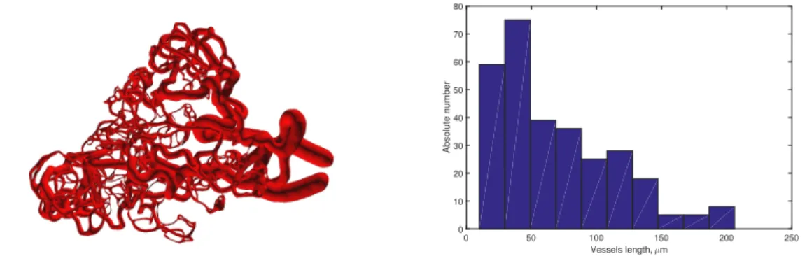
0 50 100 150 200 250
Vessels length, µm 0
10 20 30 40 50 60 70 80
Absolute number
Figure 3.Left: An artificially generated 3D blood vessel network (for a sphere with a diameter of about 200
µm). Right: Vessels length distribution of the computationally constructed blood microvascular model.
The blood microvascular network generated using the developed algorithm is shown in Figure3.
3.4. Integrative Geometric Model of Vascular Networks
Figure 4.FRC network 3D model (for sphere with a diameter of about 200µm)
Figure 5. FRC network. Left: Network graph. Center: Node degree distribution. Right: Edges lengths distribution.
The method developed in [7] was further utilized to place two or more network graphs in same domain. To this end, we placed both graph structures in one structure, unified the length of all edges (we converted them into sets of edges with length about 4 µm) and executed the minimisation of length inconsistencies using a modified version of the algorithm from [7]. Some remaining intersections were removed at the stage of voxel-based approximation of the graphs. The key characteristics of the constructed 3D blood microvascular model are listed in Table2:
Table 2.Constructed 3D models options
FRCn Vascular network Surface area 1131209µm2 61264µm2
Relative volume 7.98% 1.71%
Figure 6.Integrated model of vascular vessels and and FRC network (for a sphere of about 200µm)
additional operations (voxel approximation, smoothing of the 3D surface) requires about 2 hours CPU time.
4. Lymph Dynamics in Conduit Elements of FRC Network
In this section we examine generic conduit and the FRC network properties.
4.1. Transport Through a Single Conduit
FRC network conduits consist of reticular fibres arranged in bundles encased by FRCs [30]. These conduits have been observed with radii between 200nm and 3µm [35], consisting of 10-100 reticular fibres[36] with radii of 20-40nm [37]. Microscopy of FRC conduits appear to show that the fibres are densely packed [36]. Lagrange found the optimal packing of cylinders is hexagonal with a maximum fibre density ofφ = π
2√3. There is some justification for the assumption that FRC conduits consist of
FRC
Collagen
Flow Channel
2rf π
3
Flow Channel
Figure 7.Diagram showing the packaged bed model of an FRC conduit. Reticular fibres are hexagonally close packed and encased in FRCs.rfis the radius of the fibres.
The cross section of the path available for flow between three fibres is bound by threeπ
3 arcs together
forming the flow boundary,Γ. The area of the section bound by the fibres is the flow domain,Ω. The area of this domain,Ap, can be found by subtracting the area of the circular sections from the area of the
triangle shown in Fig7.
Ap=r2f
√
3−π
2
(5)
The Navier-Stokes equation for incompressible, steady-state, unidirectional flow of a Newtonian fluid reduces to a Poisson equation and can be written as below.
∇2u= pz
µ (6)
Whereuis the velocity,µthe viscosity andpzis thezaxis component of the pressure gradient. Using a
finite element solver with a no-slip boundary conditionu(Γ) =0. An area independent flow parameter, χ, is defined as follows,
χ= A2p
Q pz
µ (7)
A finite element solver was used the find χ for curvilinear triangular domains such as Ω. The area independence ofχwas verified and a convergence study performed, the results are tabulated below.
A rearrangement of eq.7gives the flow in one of theΩdomains for a given pressure gradient in the formQR=pzwithRdefined as ,
R= χµ
A2
p
(8)
Based on the values found for χ it is observed that the resistance value found for flow through a curvilinear triangular cross-section is twice that through a circular cross-section of the same area. The total resistance,Rtot, for a conduit containing multiple fibrils is the reciprocal of the sum of the reciprocal
Degree of Freedom χ
16 49.4300
64 50.1578
256 49.8887
1024 49.7000
4096 49.7130
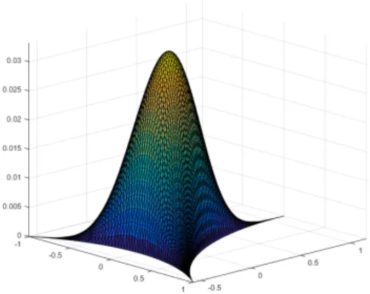
Figure 8.Left: Table of area independent parameterχagainst degrees of freedom in the FEA model. Right:
Numerically computed velocity profile of flow through a curvilinear triangle with areaAp.
4.2. Diffusive Transport in an FRC conduit
At scales such as these diffusive mass transport can be considerably more significant than fluid flow. The geometry of the channels seems that it will produce large viscous losses whilst still retaining a large cross-sectional area available for transport. Assuming ideal mixtures a relationship (Fick’s law) can be constructed for mass diffusion within the conduits in a similar manner,
− N l
DA =∆C (9)
where∆Cis the difference in molar concentration,Nis the molar flux andDis the diffusivity. Now if we assume a 300µmlong pipe spanning a lymph node with a pressure difference of 6cmH2Oand a viscosity
of 1.5cp [38] then the Péclet number in a conduit is 0.0388 - for diphtheria toxin, see below - suggesting its motion is diffusion dominated. Thus it is reasonable to assume the flow will have an insignificant effect on the concentration of diphtheria toxin allowing these two transport phenomena to be decoupled.
Instead of a 3D fluid solver operating on a void space of the network, a 0D solver can operate on the connectivity and associated properties of the network with a considerable reduction in computational expense. Such a solver was implemented in MATLABR and a cuboid block of a generated FRC network
consisting of 6927 edges and 3374 nodes was subjected to analysis. Contiguous nodes were made co-planar to give a domain of known dimensions, 151×193×187µm. Pressure or concentration gradients were placed across the block, a linear system formed and solved for the fluid permeability or diffusive flux using a direct solver. One species often considered in lymphatics is diphtheria toxin with a diffusivity D = 6.2∗10−7 cm/s[39] and a molecular weight of 58kDa[40]. For the network under consideration a
5. Modelling Lymph Flow in Conduit System of FRC Network in Idealized LN
5.1. Normal FRC network
In order to simulate a steady-state lymph flow in a conduit system of the FRC network model in an idealized LN designed in [7], we applied Poiseuille law as well as mass conservation law. Let’s consider the graph of conduit network shown in Figure4and denote set of vertices and edgesG= (V,E). For each edgeeij ∈Ewe apply the Poiseuille equation and for each vertexvi∈Vwe apply the mass conservation
law (i,j=1, 3694).
Qij=
1 Rij
Pi−Pj
∑
ki:iki∈E
Qiki =0 (10)
The variables are the lymph flowQij[(µm)3/s], the hydraulic pressurePi[Pa] and hydraulic resistance,Rij.
According the Poiseuille equation, hydraulic resistance for non-elastic tubes is the following:R= 8µl πr4 The
parameterµ=0.0015 Pa·s is the lymph dynamic viscosity [32]. The radiirijof all channels are assumed
to have a constant value of 1µm. Channel lengthslijcan be calculated from graph data shown in Figure
4. If we take into consideration reticular fibres densely packed in conduits and use hydraulic resistance defined in equation8, the flow through the system will be about 7 orders lower.
Qf ibres
Qtube =
Rtube
Rf ibres =
8µ/πr4c µχ/(
√
3−π
2)2r4f
'1.33·10−7 (11)
The system10needs to be closed by setting boundary conditions. The conduit network is connected
Gradient Constant
Pmax
Pmin
x
Af
Ef
.
Figure 9.Schematic view of the SCS pressure distribution for two types of pressure boundary conditions ((1) gradient and (2) constant. Branches emanating from the inner SCS circle represent the input and output edges of the network
pressure values. The first variant of pressure distribution is called «Gradient» with a linear decline from Pmax = 500 Pa to Pmin = 0 Pa depending on x-coordinate. The pressure estimates are based on values
reported in [3,6,33]. The second variant is referred by term «Constant». If we set a plane normal to the x-axis dividing the LN into two halves of equal length, points in the upper half will have a value ofPmax
and points in the lower half will havePmin.
Having specified the boundary conditions, we build a linear system, excluding the flow variables from equation 10, and solve it for pressure. The system matrix is sparse but nonsingular so we use UMFPACK solver[34] which provides a direct method for linear sparse systems. The following results have been calculated using the UMFPACK direct method. The inflow and outflow were tested to be equal, the conservation of mass condition is satisfied. A network consisted of 3694 vertices and 7253 edges with the number of input and output vertices 169 to 151 in the «gradient» case, and 164 to 156 in the «constant» case.
0.0 0.2 0.4 0.6 0.8 1.0
Relative coordinate
0 100 200 300 400 500
Pr
essu
re
, P
a
a: 0%
0.0 0.2 0.4 0.6 0.8 1.0
Relative coordinate
0 100 200 300 400 500
Pr
essu
re
, P
a
a: 0%
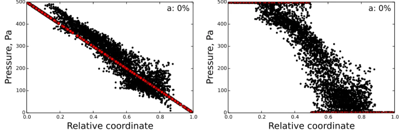
Figure 10.Pressure values depending on coordinate (a) for gradient boundary conditions. (b) for constant boundary conditions. Boundary points are highlighted in red.
Figure10demonstrates the change of pressure with growth of distance from the afferent lymphatic vessel for all vertices with different boundary conditions. In case of the gradient boundary condition (10a) there is an evident linear gradient with a line of boundary points from which others deviate slightly. In case of the constant boundary condition the pressure gradient is obviously higher, but still the pattern is close to linear.
5.2. Disrupted FRC network
Viral infections suffered by the immune system can destroy parts of the FRC network and lead to its disruption [8,14]. We applied the model of lymph flow in the conduit system to parameterize the destruction process and study its effect on lymphatic system function. To simulate a disrupted conduit system we delete edges from E randomly. If all edges connected to a node are deleted it becomes isolated, with zero pressure. Deletion of edges also leads to broken chains and pendant (or leaf) vertices. Mass conservation law implies that there is no flow into pendant vertex and no flow through broken chains. Some edges which are not removed may have no flow and so disfunction, we call these edges non-functional («n-f edges»). For example, in Figure 11illustrating the disruption elements vertices 2 and 3 are pendant, edges (1-2) and (3-8) are non-functional, vertex 6 – isolated.
1
2 3
4 5
6 7
8 1
2 3
4 5
6 7
8
nf nf
rm
rm rm
Figure 11.Scheme of edges deletion from graph
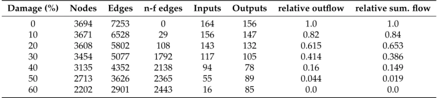
inputs and outputs with nonzero inflow and outflow (inputs and outputs are boundary nodes through which lymph flows in and out of the LN). In the tables only non-isolated nodes are counted, that’s why the number of vertices, inputs and outputs decreases. We also calculated the summary flow out of the LN (equal to the flow into the LN) and total flow through all system channels. In the tables we show a fraction of flow through the damaged system to the flow through initial undamaged system.
Table 3.System degradation for constant boundary conditions
Damage (%) Nodes Edges n-f edges Inputs Outputs relative outflow relative sum. flow
0 3694 7253 0 164 156 1.0 1.0
10 3671 6528 29 156 147 0.82 0.84
20 3608 5802 108 143 132 0.615 0.653
30 3454 5077 1792 117 105 0.414 0.386
40 3135 4352 2138 94 78 0.16 0.149
50 2713 3626 2365 55 89 0.044 0.019
60 2202 2901 2443 16 85 0.0 0.0
Table 4.System degradation for gradient boundary conditions
Damage (%) Nodes Edges n-f edges Inputs Outputs relative outflow relative sum. flow
0 3694 7253 0 169 151 1.0 1.0
10 3671 6528 27 157 146 0.854 0.845
20 3608 5802 110 140 135 0.678 0.66
30 3454 5077 226 109 113 0.49 0.398
40 3135 4352 346 85 87 0.33 0.23
50 2713 3626 454 68 76 0.26 0.149
60 2202 2901 599 46 55 0.185 0.095
70 1623 2176 512 34 41 0.135 0.074
80 1062 1451 254 13 25 0.072 0.039
90 513 725 76 5 13 0.028 0.013
connected components remain. That’s why there are less non-functional edges and more inputs and outputs in the «gradient» case than in «constant» case.
0.0 0.2 0.4 0.6 0.8 1.0 Relative coordinate 0 100 200 300 400 500 Pr essu re , P a a: 0%
0.0 0.2 0.4 0.6 0.8 1.0 Relative coordinate 0 100 200 300 400 500 Pr essu re , P a b: 10%
0.0 0.2 0.4 0.6 0.8 1.0 Relative coordinate 0 100 200 300 400 500 Pr essu re , P a c: 20%
0.0 0.2 0.4 0.6 0.8 1.0 Relative coordinate 0 100 200 300 400 500 Pr essu re , P a d: 30%
0.0 0.2 0.4 0.6 0.8 1.0 Relative coordinate 0 100 200 300 400 500 600 Pr essu re , P a e: 40%
0.0 0.2 0.4 0.6 0.8 1.0 Relative coordinate 0 100 200 300 400 500 600 Pr essu re , P a f: 50%
Figure 12. Pressure gradient for (a)–(f) 0% – 50% edges removed (constant boundary conditions). Boundary points are highlighted in red.
0.0 0.2 0.4 0.6 0.8 1.0 Relative coordinate 0 100 200 300 400 500 Pr essu re , P a a: 0%
0.0 0.2 0.4 0.6 0.8 1.0 Relative coordinate 0 100 200 300 400 500 Pr essu re , P a b: 10%
0.0 0.2 0.4 0.6 0.8 1.0 Relative coordinate 0 100 200 300 400 500 Pr essu re , P a c: 20%
0.0 0.2 0.4 0.6 0.8 1.0 Relative coordinate 0 100 200 300 400 500 Pr essu re , P a d: 30%
0.0 0.2 0.4 0.6 0.8 1.0 Relative coordinate 0 100 200 300 400 500 Pr essu re , P a e: 40%
0.0 0.2 0.4 0.6 0.8 1.0 Relative coordinate 0 100 200 300 400 500 Pr essu re , P a f: 50%
0.0 0.2 0.4 0.6 0.8 1.0 Relative coordinate 0 100 200 300 400 500 Pr essu re , P a g: 60%
0.0 0.2 0.4 0.6 0.8 1.0 Relative coordinate 0 100 200 300 400 500 Pr essu re , P a h: 70%
0.0 0.2 0.4 0.6 0.8 1.0 Relative coordinate 0 100 200 300 400 500 Pr essu re , P a i: 80%
Figures 12,13 demonstrate the difference of pressure-coordinate dependance for graphs with consequently removed edges (pressure in isolated nodes is zero).
6. Percolation Robustness of the FRC Network
6.1. Graph Measures
From graph theory there are several observations and quantitative metrics that can be made of an FRC network that imply aspects of its function. Firstly, hierarchy, which can be defined as the imbalance between the number of nodes of a low degree and the number of nodes of a high degree. A network can have more lower degree nodes than higher degree nodes by adopting “hub and spoke” features where some higher degree “hub” nodes connect to many lower degree nodes. This is indicative of a scale-free network where the degree distribution is approximately that of a power law[41]. Currently, studies of FRC networks have found a Gaussian degree distribution indicating an absence of “hubs". A more formal definition can be used to explore this through two numbers; the mean local clustering coefficient,C, as defined by Watts-Strogatz and the mean shortest path lengthL.Cican be defined for each node,i, by the
number of neighbours ofi,N(i), which are also neighbours of each other,|N(i)∩N(N(i))|and the total number of neighbours,k(i)[42].
Ci=
|N(i)∩N(N(i))|
k(i)(k(i)−1) (12)
We can now defineC as the average ofCfor all i, i.e. the average occupancy of connections between neighbours. IfL(i,j)can be defined as the shortest possible path between two nodesi,j. ThenLcan be defined as,
L= 1
n(n−1)
n
∑
i n
∑
j6=i
L(i,j) (13)
Wherenis the number of nodes in the network. In lattice type networks the mean shortest path length is relatively long compared to random networks as is the clustering coefficient. Small-world networks are defined by their small mean shortest path length whilst still maintaining the high clustering coefficient of a lattice. In order to compare networks dimensionless forms of these numbers are defined.
ˆ C= C
CER
and Lˆ = L
LER
(14)
Where the LER and CER forms of L and C are the quantities calculated on an equivalent Erdös-Rényi
random networks. Erdös-Rényi equivalent random networks have the same number of edges on the same vertices, as the network, but with edges having an equal probability of existance between all vertices. From this the small-worldness quantity,σcan be defined as the ratio of the two[42].
σ= ˆ C ˆ
L (15)
by spatially homogenising at "hubs" which will connect to a large number of "spokes". Maintenance of gradients between these spokes will be impeded by the "hub" compared to a lattice type network were in the absence of "hubs", a regular structure would exist between the "spokes". More complex gradients can exist across this regular structure than across a "hub", anode with a singular value. A greater understanding of the FRC network and the spatial variance of these quantities could allow more representative FRC networks to be generated.
6.2. Percolation Threshold
If each bond within a network has a probability,p, that it exists then the percolation threshold,pc,
is the value for p below which a spanning tree cannot exist. That is the point at which the networks connectivity is sufficiently damaged that it is not possible to move across the network. At this point the largest spanning tree remaining is a fractal object which scales with the total size of the network according to a power law[43].
The percolation threshold for this network was found to be 0.32 with a standard deviation of 0.0825 which is close to thepcof a face centred cubic, 0.119. The network under consideration was subjected to
a flow solver as described in Section4.2in order to study how fluxes change as p → pc. For each case
the flux across the network was calculated, after which an edge was removed. This process was repeated until the flux was zero. 100 cases were run and the range and standard deviation for relative change in flux are shown below in Fig.14.
Figure 14.The change in flux asp→pc.
As both viscous and diffusive effects have the same dependance on length the relationship shown in Fig.14 is true of both diffusion and fluid flux. The high pc suggests a high degree of topological
are of considerable importance to flow. Verifying the existence of these properties in nature and correctly replicating them in artificial networks will be challenging.
7. Discussion
In this study we developed computational algorithms for modelling the geometry of two transport systems of the LN, i.e., the FRC network and the microvascular network. The first one provides the structure for lymph flow through the internal parts of the LN as well as cell migration. The blood vascular networks provide access for lymphocytes from the circulation to the LN parenchyma. As the remodelling of the networks takes place during infections, it is important to map the dynamic structure of the networks to their function in terms of cellular and information molecules (cytokines, antigens, etc.,) transport and distribution within the LN. The application of experimental imaging of internal LN structures is limited in humans. Therefore, computational modeling provides the tools for predicting the relationships between geometric and topological properties of the networks as well as on their performance under homeostatic and pathological conditions.
Capturing the 3-dimensional organization of LNs presents a challenge for existing imaging and analysis systems [21]. Recent studies provide basic information about geometrical and topological properties of the LN vascular systems. We used the data on organ-wide 3D-imaging of the microvascular network in murine LNs [21] to develop a voxel-based algorithm for 3D geometric modelling of the LN blood vascular network consistently with the data on blood vessels length distribution. A Cellular Potts Modelling framework was used to develop the FRC network model meeting the constraints on the volume and properties of FRCs. The blood microvascular- and the FRC network models were embedded into the SCS of the LN modeled as a sphere with the diameter about 200µm. Taking together these two transport modules can be used to build up structurally complete computational models of the LNs as compared to those presented in [3,5,6]
To our knowledge, this is the first study in which the lymph flow through the conduit network was studied under a range of physiological conditions. The FRC network can be severely destroyed during viral infection leading to immune deficiency [8]. It has been shown recently that an FRC network can tolerate a loss of approximately 50% of their FRCs without substantial impairment of immune cell recruitment, intranodal T cell migration, and dendritic cell-mediated activation of antiviralCD8+T cells [14]. To evaluate the robustness of the conduit system in terms of the lymph percolation parameter, we have examined the lymph flow through the conduit network for an idealized geometry and under specified boundary conditions. The model based on a steady state Poiseuille equation predicts that the elimination of up to 60−90 % of edges is required to stop the lymph flux. This result suggests a high degree of the functional robustness of the network. We consider an idealised lymph node.
the model network graph embedded into metric space, i.e. having realistic edge lengths distribution according to the real FRC network data. To this end we evaluated the shortest path length to be a real physical path length. Earlier, in [44] it was shown that the small-world parameter scales linearly with network size, for both model and real-world networks. The estimate of small-worldness parameter σ=6.128 for murine FRC network data is based on the observed FRC network in T cell zone with about 170 nodes. In the model network for the entire lymph node the number of nodes is 3374, i.e., about 20-fold larger. The increase in the network size (the number of nodes) results in a proportional increase in the value small-world parameter, i.e. up to 83.1, consistently with the demonstration of the above cited study. These differences and their implications for flow and transport require further investigation. Finally, in an earlier study [45] it has been shown that fluid flow in turn regulates the reticular cell network, suggesting that models of the LN fluid homeostasis should consider elaborate feedbacks. LNs are characterized by complex multi-scale structures which represent critical issues in computational modelling of the LN physiology. Here we presented a consistent approach to integrating the blood microvascular- and the conduit network models within a confined space of the LN that will be used to study how the lymph-borne information is distributed to various parts of the lymph node under normal conditions and during an immune response. Further analysis should focus on studying the fluid-structure interactions for the vascular systems in conjunction with the cellular and chemical reactions taking place in live LNs. Finally, as it was stressed by W.E. Paul [46] "...It is to the quantitative prediction of the outcome of given perturbations in the immune system that we envisage our mathematical/modeling colleagues will apply themselves".
Acknowledgments: The research was funded by the Russian Science Foundation (Grants 14-31-00024 and 15-11-00029 (Sect. 3.1)).
Author Contributions:
• Conceived and designed the study: R.vL., I.S., G.B.;
• Performed the wet experiments and analyzed the data: M.N., L.O.;
• Developed the models and performed the computations: D.G. (Sect. 3.1), R.S. (Sect. 3.2), R.T. (Sect. 5), R.vL., I.S., D.W. (Sect. 4,6);
• Wrote the paper D.G., R.vL., M.N., R.S., I.S., R.T., D.W., G.B.
Conflicts of Interest:The authors declare no conflict of interest.
References
1. Junt, T.; Scandella, E.; Ludewig, B. Form follows function: lymphoid tissue microarchitecture in antimicrobial immune defence.Nat Rev Immunol2008, 8(10), 764-775.
2. Margaris, K.N.; Black, R.A. Modelling the lymphatic system: challenges and opportunities. J R Soc Interface 2014,9(69), 601-612.
3. Jafarnejad, M.; Woodruff, M. C.; Zawieja, D. C.; Carroll, M. C.; Moore Jr, J. E. Modeling lymph flow and fluid exchange with blood vessels in lymph nodes.Lymphatic research and biology2015,13(4), 234-247.
4. Kislitsyn, A.; Savinkov, R.;Novkovic, M.; Onder, L.; Bocharov, G. Computational Approach to 3D Modeling of the Lymph Node Geometry.Computation2015,3, 222-234.
5. Bocharov, G.; Danilov, A;.; Vassilevski, Y.; Marchuk, G.I.; Chereshnev, V.A., Ludewig, B. Reaction-diffusion modelling of interferon distribution in secondary lymphoid organs. Math Model Natural Phenomena2011, 6, 13–26.
6. Cooper, L.J.; Heppell, J.P.; Clough, G.F.; Ganapathisubramani, B.; Roose, T. An Image-Based Model of Fluid Flow Through Lymph Nodes.Bull Math Biol2016,78(1), 52-71.
8. Kumar, V.; Scandella, E. ; Danuser, R. ; Onder, L. ; Nitschke, M.; Fukui, Y.; Halin, C.; Ludewig, B.; Stein, J.V. Global lymphoid tissue remodelling during a viral infection is orchestrated by a B cell-lymphotoxin-dependent pathway.Blood2010, 115(23), 4725-4733.
9. Malhotra, D.; Fletcher, A.L.; Turley, S.J. Stromal and hematopoietic cells in secondary lymphoid organs: partners in immunity.Immunol Rev2013, 251(1), 160-176.
10. Cremasco, V.; Woodruff, M.C.; Onder, L.; Cupovic, J.; Nieves-Bonilla, J.M.; Schildberg, F.A.; Chang, J.; Cremasco, F.; Harvey, C.J.; Wucherpfennig, K.; Ludewig, B.; Carroll, M.C.; Turley, S.J. B cell homeostasis and follicle confines are governed by fibroblastic reticular cells.Nat Immunol2014, 15(10), 973-981.
11. Chang, J.E.; Turley, S.J. Stromal infrastructure of the lymph node and coordination of immunity.Trends Immunol 2015, 36(1), 30-39.
12. Chai, Q.; Onder, L.; Scandella, E.; Gil-Cruz, C.; Perez-Shibayama, C.; Cupovic, J.; Danuser, R.; Sparwasser, T.; Luther, S.A.; Thiel, V.; Rülicke, T.; Stein, J.V.; Hehlgans, T.; Ludewig, B. Maturation of lymph node fibroblastic reticular cells from myofibroblastic precursors is critical for antiviral immunity.Immunity2013, 38(5), 1013-1024. 13. Fletcher, A.L.; Acton, S.E.; Knoblich, K. Lymph node fibroblastic reticular cells in health and disease. Nat Rev
Immunol2015, 15(6), 350-361.
14. Novkovic, M.; Onder, L.; Cupovic, J.; Abe, J.; Bomze, D.; Cremasco, V.; Scandella, E.; Stein, J.V.; Bocharov, G.; Turley, S.J.; Ludewig, B. Topological Small-World Organization of the Fibroblastic Reticular Cell Network Determines Lymph Node Functionality.PLoS Biol2016, 14(7), e1002515.
15. Luther, S.A.; Tang, H.L.; Hyman, P.L.; Farr, A.G.; Cyster, J.G. Coexpression of the chemokines ELC and SLC by T zone stromal cells and deletion of the ELC gene in the plt/plt mouse. Proc Natl Acad Sci U S A2000, 97(23), 12694-12699.
16. Link, A.; Vogt, T.K.; Favre, S.; Britschgi, M.R.; Acha-Orbea, H.; Hinz, B.; Cyster, J.G.; Luther, S.A. Fibroblastic reticular cells in lymph nodes regulate the homeostasis of naive T cells.Nat Immunol2007, 8(11), 1255-1265. 17. Mueller, S.N.; Germain, R.N. Stromal cell contributions to the homeostasis and functionality of the immune
system.Nat Rev Immunol2009, 9(9), 618-629.
18. Sixt, M.; Kanazawa, N.; Selg, M.; Samson, T.; Roos, G.; Reinhardt, D.P.; Pabst, R.; Lutz, M.B.; Sorokin, L. The conduit system transports soluble antigens from the afferent lymph to resident dendritic cells in the T cell area of the lymph node.Immunity2005, 22(1), 19-29.
19. Onder, L.; Danuser, R.; Scandella, E.; Firner, S.; Chai, Q.; Hehlgans, T.; Stein, J.V.; Ludewig, B. Endothelial cell-specific lymphotoxin-βreceptor signaling is critical for lymph node and high endothelial venule formation.
J Exp Med2013, 210(3), 465-473.
20. Girard, J.P.; Moussion, C.; Förster, R. HEVs, lymphatics and homeostatic immune cell trafficking in lymph nodes.Nat Rev Immunol2012, 12(11), 762-773.
21. Kelch, I.D.; Bogle, G.; Sands, G.B.; Phillips, A.R.; LeGrice, I.J.; Dunbar, P.R. Organ-wide 3D-imaging and topological analysis of the continuous microvascular network in a murine lymph node.Sci Rep2015, 5:16534. 22. Subramanian, N.; Torabi-Parizi, P.; Gottschalk, R.A.; Germain, R.N.; Dutta, B. Network representations of
immune system complexity.Wiley Interdiscip Rev Syst Biol Med2015, 7(1), 13-38.
23. Heng, T.S.; Painter, M.W.; Immunological Genome Project Consortium. The Immunological Genome Project: networks of gene expression in immune cells.Nat Immunol2008, 9(10), 1091-1094.
24. Kitano, H. Systems Biology: a brief overview.Science2002, 295, 1662-1664.
25. Ludewig, B.; Stein, J.V.; Sharpe, J.; Cervantes-Barragan, L.; Thiel, V.; Bocharov, G. A global “imaging” view on systems approaches in immunology. EurJ Immunol2012, 42(12), 3116-3125.
26. Glazier, J.A.; Balter, A.; Poplawski, N.J. Magnetization to morphogenesis: a brief history of the Glazier-Graner-Hogeweg model. In Single-Cell-Based Models in Biology and Medicine; Anderson, A.R.A.; Chaplain, M.A.J.; Rejniak, K.A.; Mathematics and Biosciences in Interactions, Birkaüser: 2007; pp. 79-106. 27. Balter, A.; Merks, R.M.H.; Poplawski, N.J.; Swat, M.; Glazier, J.A. The Glazier-Graner-Hogeweg model:
28. Marée, A.F.M.; Grieneisen, V.A.; Hogeweg, P. The Cellular Potts Model and biophysical properties of cells, tissues and morphogenesis. InSingle-Cell-Based Models in Biology and Medicine; Anderson, A.R.A.; Chaplain, M.A.J.; Rejniak, K.A.; Mathematics and Biosciences in Interactions, Birkaüser: 2007; pp. 107-136.
29. Scianna, M.S.; Preziosi, L.P. Multiscale Developments of the Cellular Potts Model. SIAM Journal on Multiscale Modeling and Simulation2012,10(2), 1-43.
30. Roozendaal, R.; Mebius, R.E.; Kraal, G. The conduit system of the lymph node. Int Immunol2008, 20(12), 1483-1487.
31. Merks, R.M.; Brodsky, S.V.; Goligorksy, M.S.; Newman, S.A.; Glazier, J.A. Cell elongation is key to in silico replication of in vitro vasculogenesis and subsequent remodeling.Dev. Biol.2006,289(1), 44-54.
32. Swartz, M.A.; Fleury, M.E. Interstitial flow and its effects in soft tissues. Ann Rev Biomed Engineer 2007, 9,229–256.
33. Bouta, E.M., Wood, R.W., Brown, E.B., Rahimi, H., Ritchlin, C.T., Schwarz, E.M. In vivo quantification of lymph viscosity and pressure in lymphatic vessels and draining lymph nodes of arthritic joints in mice.J Physiol2014, 92(6), 1213-23.
34. UMFPACK: http://faculty.cse.tamu.edu/davis/suitesparse.html
35. Delves, P., Martin, S., Burton, D., Roitt, I., Roitt’s Essential Immunology. Somerset: Wiley. 2011; 239.
36. Gertz, J. E., Anderson, A. O., Shaw, S., Cords, channels, corridors, conduits: critical architectural elements facilitating cell interaction in the lymph node cortex.Immunol Rev1997, 156, 11-24.
37. Ushiki, T. Collagen Fibers, Reticular Fibers and Elastic Fibers. A Comprehensive Understanding from a Morphological Viewpoint.Arch Histol Cytol2002, 65(2), 109-206.
38. Swartz, M.A., Fleury, M.E., Interstitial flow and its effects on soft tissue.Annu Rev Biomed Eng2007, 9, 229-256. 39. Pappenheimer Jr., A.M., Lundgren, H.P., Williams, J.W., Studies on the Molecular Weight of Diphtheria Toxin,
Antitoxin and their Reaction Products.J Exp Med1939, 71(2), 247-62.
40. Wolffa, C., Wattiezb, R., Jean-Marie Ruysschaerta, J., Cabiauxa, V., Characterization of diphtheria toxin?s catalytic domain interaction with lipid membranes.Biochimica et Biophysica Acta2004, 1611, 166-177.
41. Rodrigue, J.P., Comtis, C., Slack, B., The Geography of Transport Systems. Hofstra University Press. 2013; 60-70. 42. Humphries, M.D., Gurney, K., Network ’Small-World-Ness’: A Quantitative Method for Determining
Canonical Network Equivalence.PLOS One2008, 3(4), e0002051.
43. Stauffer, D., Aharony, A., Introduction to percolation theory. CRC press. 1994.
44. Humphries, M.D.; Gurney, K. Network ’small-world-ness’: a quantitative method for determining canonical network equivalence.PLoS One2008, 3(4), e0002051.
45. Tomei, A.A.; Siegert, S.; Britschgi, M.R.; Luther, S.A.; Swartz, M.A. Fluid flow regulates stromal cell organization and CCL21 expression in a tissue-engineered lymph node microenvironment.J Immunol2009, 183(7), 4273-83. 46. Paul, W.E., The immune system—complexity exemplified. Mathematical Modelling of Natural Phenomena2012,
7(5), 4–6.
Abbreviations
The following abbreviations are used in this manuscript: FRC: Fibroblastic reticular cell
SCS: Subcapsular sinus LN: lymph node
c
![Figure 2. Blood vessels length distribution summarized from [ 21 ]](https://thumb-us.123doks.com/thumbv2/123dok_us/8011936.1331949/6.918.289.620.654.882/figure-blood-vessels-length-distribution-summarized.webp)