Application of a Convolutional Neural Network for image
classification for the analysis of collisions in High Energy
Physics
CeliaFernández Madrazo1,IgnacioHeredia1,∗,LaraLloret1, andJesúsMarco de Lucas1 1Instituto de Física de Cantabria, IFCA (CSIC-UC)
Abstract.The application of deep learning techniques using convolutional neu-ral networks for the classification of particle collisions in High Energy Physics is explored. An intuitive approach to transform physical variables, like mo-menta of particles and jets, into a single image that captures the relevant in-formation, is proposed. The idea is tested using a well-known deep learning framework on a simulation dataset, including leptonic ttbar events and the cor-responding background at 7 TeV from the CMS experiment at LHC, available as Open Data. This initial test shows competitive results when compared to more classical approaches, like those using feedforward neural networks.
1 Introduction
Deep learning with convolutional neural networks (CNNs) has revolutionized the world of computer vision and speech recognition over the last few years, yielding unprecedented per-formance in many machine learning tasks and opening a wide range of possibilities [1].
In this paper, we explore a particular application of CNNs, image classification, in the context of analysis in experimental High Energy Physics (HEP). Recent work has already successfully applied many ideas of the deep learning community to the HEP field [2]. Many studies in this field, including the search for new particles, require solving difficult signal-versus-background classification problems, hence machine learning approaches are often adopted. For example, Boosted Decision Trees [3] and Feedforward Neural Networks [4] are much used in this context, but the latest state-of-the-art methods have not yet been fully explored and can bring a new light on the torrent of data being generated by experiments like those at the Large Hadron Collider (LHC) at CERN.
In a first approach, we have tested the use of convolutional networks for the classification of collisions at LHC using Open Data Monte Carlo samples. The Compact Muon Solenoid (CMS) experiment [5] has pioneered, in the context of the LHC, in publicizing the collision data collected by the detector to the international community in order to carry out new analy-ses or to use them for training activities. CMS Open Data is available from the CERN Open Data portal1and we also have a dedicated portal developed in our center2.
In order to apply deep learning techniques developed for image classification for the anal-ysis of these collisions, we propose an innovative visual representation of the different physics
∗e-mail: [email protected]
observables. We train a convolutional neural network on these visual representations, repre-senting simulated proton-proton collisions, to try to distinguish a particular physics process of interest. In our example, we try to distinguish the production of a pair of quarks top anti-top (ttbar) from other processes (background).
2 Methods
2.1 Deep Learning Architecture
The technique of image classification using CNNs is included in the scope of deep learning. Deep learning is part of a broader family of machine learning methods based on learning data representations, as opposed to task-specific algorithms. The performance of these processes depends heavily on the representation of the data and the algorithm used [6].
Following previous successful work in other fields within our group (i.e. identifying plants [7]), we have selected as CNN architecture the Residual Network model [8] (ResNet) which won the ImageNet Large Scale Visual Recognition Challenge in 2015 [9].
The architecture of the ResNet model used consists of a stack of similar (so-called resid-ual) blocks, each block being in turn a stack of convolutional layers. The innovation of this architecture is that the output of a block is also connected with its own input through an iden-tity mapping path. This alleviates the vanishing gradient problem, improving the gradient backward flow in the network and allowing to train much deeper networks. We choose our model to have 50 convolutional layers (aka. ResNet50).
As deep learning framework, we use the Lasagne [10] module built on top of Theano [11][12]. We initialize the weights of the model with the pretrained weights on the ImageNet dataset provided in the Lasagne Model Zoo. We train the model for 40 epochs on different top-performing GPUs using the Adam [13] optimizer. During training, we apply standard data augmentation (as sheer, translation, mirror, etc), and after we apply the transformations, we downscale the image to the ResNet standard input size (224×224 pixels)3. The training took around one day on a single NVIDIA GTX 1080 Ti.
2.2 Dataset
The overall pipeline in CNNs is similar to standard NNs except for the fact that in this case we feed an image represented by a 3 dimensional tensor of shapeH×W×C, whereHstands for image height (here equal to 224),W stands for image width (here equal to 224) andC stands for the number of channels (here equal to 3, the RGB values). As in most machine learning algorithms, in this workflow we divide the image data in three splits (train|val|test) with roughly (70|15|15) % of the images as shown in Table 1.
We will use events corresponding to Monte Carlo simulated collisions at 7 TeV at LHC recorded by the CMS detector [14], that have been released as Open Data by the CMS col-laboration.
The preprocessing of the samples and the image generation has been done in Python4and took around one day. The images have been generated extracting the simulated collisions data from a dedicated JSON file containing the main information on the physics observables at play. The JSON has been produced using a C++framework5based on a template provided by the Open Data group to which the JSON generation part has been added. An example of
observables. We train a convolutional neural network on these visual representations, repre-senting simulated proton-proton collisions, to try to distinguish a particular physics process of interest. In our example, we try to distinguish the production of a pair of quarks top anti-top (ttbar) from other processes (background).
2 Methods
2.1 Deep Learning Architecture
The technique of image classification using CNNs is included in the scope of deep learning. Deep learning is part of a broader family of machine learning methods based on learning data representations, as opposed to task-specific algorithms. The performance of these processes depends heavily on the representation of the data and the algorithm used [6].
Following previous successful work in other fields within our group (i.e. identifying plants [7]), we have selected as CNN architecture the Residual Network model [8] (ResNet) which won the ImageNet Large Scale Visual Recognition Challenge in 2015 [9].
The architecture of the ResNet model used consists of a stack of similar (so-called resid-ual) blocks, each block being in turn a stack of convolutional layers. The innovation of this architecture is that the output of a block is also connected with its own input through an iden-tity mapping path. This alleviates the vanishing gradient problem, improving the gradient backward flow in the network and allowing to train much deeper networks. We choose our model to have 50 convolutional layers (aka. ResNet50).
As deep learning framework, we use the Lasagne [10] module built on top of Theano [11][12]. We initialize the weights of the model with the pretrained weights on the ImageNet dataset provided in the Lasagne Model Zoo. We train the model for 40 epochs on different top-performing GPUs using the Adam [13] optimizer. During training, we apply standard data augmentation (as sheer, translation, mirror, etc), and after we apply the transformations, we downscale the image to the ResNet standard input size (224×224 pixels)3. The training took around one day on a single NVIDIA GTX 1080 Ti.
2.2 Dataset
The overall pipeline in CNNs is similar to standard NNs except for the fact that in this case we feed an image represented by a 3 dimensional tensor of shapeH×W×C, whereHstands for image height (here equal to 224), W stands for image width (here equal to 224) andC stands for the number of channels (here equal to 3, the RGB values). As in most machine learning algorithms, in this workflow we divide the image data in three splits (train|val|test) with roughly (70|15|15) % of the images as shown in Table 1.
We will use events corresponding to Monte Carlo simulated collisions at 7 TeV at LHC recorded by the CMS detector [14], that have been released as Open Data by the CMS col-laboration.
The preprocessing of the samples and the image generation has been done in Python4and took around one day. The images have been generated extracting the simulated collisions data from a dedicated JSON file containing the main information on the physics observables at play. The JSON has been produced using a C++framework5based on a template provided by the Open Data group to which the JSON generation part has been added. An example of
3Code available at https://github.com/IgnacioHeredia/plant_classification 4Code available at https://github.com/CeliaFernandez/Image-Creation 5Code available at https://github.com/laramaktub/json-collisions
Table 1.Distribution of the number of images among the three classes we intend to classify for the train,validationandtestsets.
Class train set val set test set
tt¯+jets 30809 41,94% 5000 33,33% 5000 33,33% Drell-Yan 21709 29,54% 5000 33,33% 5000 33,33%
W+jets 20950 28,52% 5000 33,33% 5000 33,33%
Total 73468 15000 15000
the JSON file format used (short.json) together with the instructions to run the code can also be found in the repository.
We have chosen as physics channel the production of top quark pair events, where each top quark decays into a W boson and a bottom quark. We want to select collisions where one of the W bosons decays leptonically into a charged lepton, electron or muon, with an associated neutrino. Although complex, these events provide a clear experimental signature, with an isolated lepton with high-transverse momentum, hadronic jets and a large missing transverse energy. We have considered as background processes the production of events where a W boson is produced in association with additional jets (W+jetsevents) and events corresponding to the so calledDrell-Yanprocesses. The CMS publication webpage6on top physics results at 7 TeV provides a description of the interest of this physics analysis channel and detailed presentations of the involved processes, methods and results. All three samples [15][16][17] are obtained from the CMS Open Data portal.
We will focus on events having one lepton with a transverse momentum greater than 20 GeV fulfilling all the standard quality criteria for isolation and identification. We select jets with a transverse momentum,pT, greater than 30 GeV and within the angular range defined by|η|<2.4. We apply a b quark tagging discriminant (b-tagging), allowing us to identify (or "tag") jets originating from bottom quarks, by using the Combined Secondary Vertex (CSV) which is based on several topological and kinematical secondary vertex related variables as well as information from track impact parameters. We also use and represent in the event images the Missing Transverse Energy (MET).
2.3 Representing Particle Collisions as Images
The main innovation of this work is the way in which the collisions are represented as images. Collisions, also known as events, recorded in a HEP experiment by a detector like CMS [14], are described by a set of variables measured corresponding to the particles detected: the momentum of muons, electrons, photons and hadrons produced in the collision of the two accelerated protons, that are determined by the different subdetectors (tracking system, calorimeters, muon system, etc.). Along the global reconstruction of the event, new variables like the definition and momentum of jets are also introduced. The analysis of events uses this set of variables to discriminate between the events corresponding to the physics process of interest and the events corresponding to the background. The most relevant observables in a collision correspond to the momenta (energy and direction) of the reconstructed particles or jets and other global variables like the missing energy.
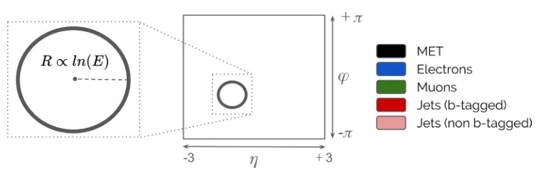
As we already mentioned, the design of the event representation is crucial when gener-ating the images for classification. All the observables are to be represented using a canvas of dimension 224×224 pixels. In our approach each particle or physics object is represented
as a circle with a radius proportional to its energy, and centered in the canvas at a position corresponding to its momentum direction. The momentum direction can be defined using two variables: the pseudorapidityη, related to the polar angle, and the azimuthal angleϕ, both of which are standard choices in experiments with cylindrical symmetry. Additionally, we associate the color of the circumference to the type of particle or physics object represented. Several considerations were taken into account when proposing this representation, namely:
• Resolution
Each physics object will be represented by a circumference with a radius defined as a function of its energy. As it is drawn using a discrete number of pixels, the scale must be chosen to accommodate the different ranges of energies while preserving as much as possible the resolution in energy.
• Out of range representation
When increasing the scale, the low energy objects can be better differentiated but circum-ferences corresponding to high energy objects could exceed the canvas size causing a mis-interpretation. This is the main reason to discard a lineal dependency with the energy.
• Overlapping
If the particles have relatively closeηandϕvalues for their momenta directions, the cor-responding representations may overlap. This is the main reason to choose circumferences instead of full circles for their representation. One future direction could be looking at full circles with some transparency and see how it compares with the current approach.
The use of a logarithmic scale to transform the energy of the physics object into a radius for the circumference representing it, allows us to reach a trade-off between the previous factors:
R=C·ln (E) (1)
where the valueCis an effective scale factor (here we choose it to be 10.5) that allows us to conciliate the previous points for the collisions being studied, providing the conversion into pixel units. The center of the circumference, also in pixels units, is obtained using conversion factors 6/224 along the η axis and 2π/224 along the ϕone, corresponding to the ranges [−3,3] forηand [−π, π] forϕ.
Figure 1 presents a diagram of this representation for a single particle. Each type of par-ticle and jet is drawn with a different color: blue for the electrons, green for the muons, light red for non-btagged jets and dark red for btagged jets. Additionally, the missing transverse energy is drawn as a black circumference in each collision, moving vertically (according to ϕMET), and horizontally centered atη =0. As before its radius scales logarithmically with the absolute value of the MET.
Figures 2(a)-2(c) show sample images from the dataset corresponding to the different classes of events under study.
3 Results
as a circle with a radius proportional to its energy, and centered in the canvas at a position corresponding to its momentum direction. The momentum direction can be defined using two variables: the pseudorapidityη, related to the polar angle, and the azimuthal angleϕ, both of which are standard choices in experiments with cylindrical symmetry. Additionally, we associate the color of the circumference to the type of particle or physics object represented. Several considerations were taken into account when proposing this representation, namely:
• Resolution
Each physics object will be represented by a circumference with a radius defined as a function of its energy. As it is drawn using a discrete number of pixels, the scale must be chosen to accommodate the different ranges of energies while preserving as much as possible the resolution in energy.
• Out of range representation
When increasing the scale, the low energy objects can be better differentiated but circum-ferences corresponding to high energy objects could exceed the canvas size causing a mis-interpretation. This is the main reason to discard a lineal dependency with the energy.
• Overlapping
If the particles have relatively closeηandϕvalues for their momenta directions, the cor-responding representations may overlap. This is the main reason to choose circumferences instead of full circles for their representation. One future direction could be looking at full circles with some transparency and see how it compares with the current approach.
The use of a logarithmic scale to transform the energy of the physics object into a radius for the circumference representing it, allows us to reach a trade-off between the previous factors:
R=C·ln (E) (1)
where the valueCis an effective scale factor (here we choose it to be 10.5) that allows us to conciliate the previous points for the collisions being studied, providing the conversion into pixel units. The center of the circumference, also in pixels units, is obtained using conversion factors 6/224 along the η axis and 2π/224 along the ϕ one, corresponding to the ranges [−3,3] forηand [−π, π] forϕ.
Figure 1 presents a diagram of this representation for a single particle. Each type of par-ticle and jet is drawn with a different color: blue for the electrons, green for the muons, light red for non-btagged jets and dark red for btagged jets. Additionally, the missing transverse energy is drawn as a black circumference in each collision, moving vertically (according to ϕMET), and horizontally centered atη =0. As before its radius scales logarithmically with the absolute value of the MET.
Figures 2(a)-2(c) show sample images from the dataset corresponding to the different classes of events under study.
3 Results
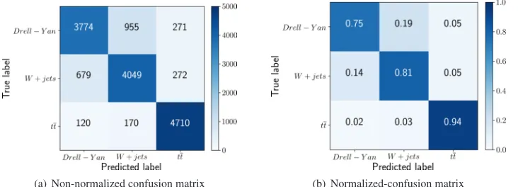
The objective is to be able to differentiate betweentt¯+jetsevents, and those corresponding toDrell-YanandW+jetsprocesses. The confusion matrix for the test set is shown in Figure 3. Approximately 94% of the pre-selected ttbar events are correctly classified, while around 5% of the W+jets and 4% of the Drell-Yan events are incorrectly tagged as ttbar. In a signal
Figure 1.Particle collisions represented as an image. Particles are represented as circumferences with radius proportional to the logarithm of their energy. The horizontal position of the particles corresponds to the pseudorapidityηwithin the range [−3, 3]. The vertical position shows the azimuthal angleϕ
within the range [−π, π].
(a)Drell-Yan (b)W+jets (c)tt¯+jets
Figure 2.Examples of images corresponding to the three different classes of collisions being classified. The x-axis depicts the pseudorapidityηwhile the y-axis depicts the azimuthal angleϕ.
(tt¯+ jets) and background (Drell-YanandW+jets) context, with 50/50 splits, the signal vs background discrimination efficiency would be 95,4%.
We have also tried training the network defining only those two categories, signal (tt¯+jets) and background (Drell-YanandW+ jets). However it results in a slightly worse classification performance with a signal vs background efficiency of 93,6%.
These results have been compared with those obtained by using a simpler, more direct, approach like deep feedforwardneural networks (FNNs). Here we use a net of 5 hidden layers with 500 units per layers and standard 50% dropout [18] between layers. The confusion matrix is shown in Figure 4. As we can see comparing it to Figure 3, FFNs are better at classifyingtt¯+jetsandW+jets(but notDrell-Yan). However, more importantly, we can see that CNNs would outperform FFNs in the signal vs background metric, with a 94,6% efficiency for FFNs.
(a) Non-normalized confusion matrix (b) Normalized confusion matrix
Figure 3.Confusion matrices for the test set using convolutional neural networks.
(a) Non-normalized confusion matrix (b) Normalized-confusion matrix
Figure 4.Confusion matrices for the test set case using feedforward neural networks.
The downside of FNNs is their vector representation of variables, which makes handling heterogeneous (non fixed-size) data not very intuitive. In this case we handled the various length events by filling the empty parameters with default values. In contrast, in the CNN case, adding one more particle to the event is as simple as drawing one more circle in the image.
An extensive comparison of the performance of our idea compared to other methods can be found in subsequent work [19].
4 Conclusions
The preliminary results presented in this study show that the use of Convolutional Neural Networks could be a promising tool to classify collisions in particle physics analysis. An intuitive visual representation of the events, that enables the inclusion of the main observables used in high energy physics analysis into an image, has been proposed.
This has been applied to the classification of complex events, using Open Data describing simulated collisions at LHC at 7 TeV in the CMS detector, corresponding to three different physics processes: Drell-Yan,W+ jetsandtt¯+ jets. The test has returned promising initial
results, correctly tagging signal and background events with an efficiency around 95%, and comparing slightly favourably with other more direct methods, like standard feedforward NNs. We plan to extend this work in the future to analyze, among other possibilities, its applicability to the classification of real data.
5 Acknowledgements
We would like to show our gratitude to the Open Data group in CMS for all the valuable support and for providing insight and expertise that greatly assisted the realization of this work.
References
[1] Y. LeCun, Y. Bengio, G. Hinton, Nature521, 436 (2015)
[2] P. Baldi, P. Sadowski, D. Whiteson, Nature Communications5(2014)
[3] B.P. Roe, H.J. Yang, J. Zhu, Y. Liu, I. Stancu, G. McGregor, Nuclear Instruments and Methods in Physics Research Section A: Accelerators, Spectrometers, Detectors and Associated Equipment543, 577 (2005)
[4] H. Kolanoski,Application of Artificial Neural Networks in Particle Physics(Springer Berlin Heidelberg, Berlin, Heidelberg, 1996), pp. 1–14, ISBN 978-3-540-68684-2, https://doi.org/10.1007/3-540-61510-5_1
[5] C. collaboration, Journal of Physics G: Nuclear and Particle Physics34(2007)
[6] Y. Bengio, A. Courville, P. Vincent,Representation learning: A review and new
per-spectives(2012),arXiv:1206.5538
[7] I. Heredia,Large-Scale Plant Classification with Deep Neural Networks, inProceedings
of the Computing Frontiers Conference (ACM, New York, NY, USA, 2017), CF’17,
pp. 259–262, ISBN 978-1-4503-4487-6,http://doi.acm.org/10.1145/3075564. 3075590
[8] K. He, X. Zhang, S. Ren, J. Sun,Deep residual learning for image recognition(2015), arXiv:1512.03385
[9] O. Russakovsky et al., International Journal of Computer Vision (IJCV)115, 211 (2015) [10] S. Dieleman et al.,Lasagne: First release. (2015),http://dx.doi.org/10.5281/
zenodo.27878
[11] J. Bergstra et al.,Theano: a CPU and GPU Math Expression Compiler, inProceedings of the Python for Scientific Computing Conference (SciPy)(2010), oral Presentation [12] F. Bastien et al., Theano: new features and speed improvements, Deep Learning and
Unsupervised Feature Learning NIPS 2012 Workshop (2012)
[13] D. Kingma, J. Ba, Adam: A method for stochastic optimization (2014), arXiv:1412.6980
[14] CMS Collaboration, Journal of Instrumentation3, S08004 (2008)
[15] CMS Collaboration,Simulated dataset dyjetstoll_tunez2_m-50_7tev-madgraph-tauola in aodsim format for 2011 collision data (sm inclusive)(2016),
DOI:10.7483/opendata.cms.txt4.4rrp,http://opendata.cern.ch/record/
1395
[16] CMS Collaboration, Simulated dataset wjetstolnu_tunez2_7tev-madgraph-tauola in aodsim format for 2011 collision data (sm inclusive)(2016),
DOI:10.7483/opendata.cms.u7p6.ckvb,http://opendata.cern.ch/record/
[17] CMS Collaboration,Simulated dataset ttjets_tunez2_7tev-madgraph-tauola in aodsim format for 2011 collision data (sm inclusive)(2016),
DOI:10.7483/opendata.cms.zbgf.h543,http://opendata.cern.ch/record/ 1544
[18] N. Srivastava, G. Hinton, A. Krizhevsky, I. Sutskever, R. Salakhutdinov, Journal of Machine Learning Research15, 1929 (2014)