2004 5th Asian Control Conference
Set Point Response
and
Disturbance
Rejection
Tradeoff
for Second-Order
Plus
Dead Time
Processes
Juan Shi and
Wee
Sit
Lee
School
of
Electrical Engineering
Faculty
of Science, Engineering and
Technology
Victoria University
of Technology
P.O.Box 14428,
MCMC
Melbourne
8001, Victoria, Australia
Email:
[email protected],
weesit
.leeQvu.edu.au
Abstract
'In this paper, we shall present simple and effective tun- ing formulas €or IMC controllers when they are applied to second-order plus dead-time processes (SOPDT). We have discovered that for controllers designed by applying IMC method, the proportional gain, the integml gain,
the derivative gain of the
PID
part of the controllerand un associate filter should all be modified accord- ing to the given.formulas for
the
purpose of achieving set-point response and disturbance rejection tradeoff.The study has also shown that the tradeoff between set- point response and disturbance rejection is limited by
normalised dead time of the SOPDT processes for the simple pole cases.
1
Introduction
According to [lo], a survey carried out in Japan in 1989
revealed that proportional plus integral plus derivative (PID) controlIers were employed in more than 90%
of
the control loops. This is because PID controlIers are low order, have simple structures that are intuitively appeal- ing, and tunning methods are widely available [13].For many industrial and chemical pIants that do not have integral and resonant characteristics, the dominant process dynamics can be represented by a first-order plus dead-time (FOPDT) transfer function [5]; that is, in Fig-
ure 1.
(1)
where K is the static process gain, r
>
0 is the dominant time-constant in-seconds, and L>
0 is the apparent dead time in seconds.Many tuning formulas for PID controllers have been obtained for FOPDT processes [5, 71 by optimising some
time-domain performance criteria. It was shown in [l]
that, for FOPDT processes with a n o r m a h e d deud time
(definded as L/T) between 0.1 and
I,
many of the known tuning methods often do not produce robust closed- loop systems, with a phase margin falling short of 30" and a gain margin of less than 4dB. Since stability robustness and performance robustness are important requirements, extensive research efforts have been di- rected towards discovering robust tuning formulas for PID controllers. For example, by considering gain and phase margin requirements with the minimum integralof squared error criterion, Ho and his co-workers [2] have
successfully obtained empirical tuning formuIas through curve fitting for optimal disturbance rejection when the process input is subjected t o a step disturbance. Al- ternatively, by applying Ieast-squares reduction to con- trollers designed with the Internal Model Control (IMC)
method [4], Wang and his co-workers [SI have obtained PID controllers with good phase margin'and step set- point response. However, [2] and [B] did not provide any
guidelines on how set-point response and disturbance rejection tradeoff could be accomplished.
In [6], a first-order all-pass transfer €unction was em- ployed to interpolate the values of
cLS
at s=
0 and s = jug, where us is the specified gain crossover fre-quency. The IMC method is then applied to the ratio- nal function model of the plant to obtain analytically
a set of PID tuning formulas for the FOPDT process.
As a result, the actaal gain crossover frequency (which
8s exactly w g ) have been predicted accurately and ex- plicit formuIas for the phase margin
(to
be denoted by#m), the ratio of closed-loop bandwidth (to be denoted
by
w,)
to gain-crossover frequency, and the controller parameters in terms of w,L have been obtained. More- over, it was dso shown that, over the range of frequen- cies where the new approximation remained valid (i.e.when w,L
<
7 ~ / 3 ) , the closed-loop system will have aguaranteed phase margin of at least 60", and wc is lim- ited d e l y by L (as opposed to the commonly quoted
LIT when proportional controllers were employed ElZ]).
A
procedure for tuning theIMC-PID
controllers such that tradeoff is achieved between set-point response and disturbance rejection for FOPDT processes was also re- ported.In [3]; a generalised PID controller was presented.
This controller not only allows set-point response and disturbance rejection tradeoff to be achieved, but also possesses a guaranteed closed-loop nominal stability property. It was also illustrated by examples how gener- alised PID controllers and their associated tuning pro- cedure can be applied to control FOPDT processes.
In this paper, we shall extend some of the work re- ported in
[SI
and [3] to second-order plus dead time (SOPDT) processes. The set-point response and dis- turbance rejection tradeoff €or SOPDT processes will be discussed. A tuning procedure for the IMC-PID con- troller will be given and simulation examples will bepresented.
2
IMC Controllers
far SOPDT
Processes
2.1
IMC-PID
Controller
for
Second-
'
Order
Plant without Dead
Time
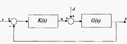
In
order to understand the constant disturbance rejec- tion property of an IMC controller for the system shown in Figure 1,
we first consider a second-order plant with- out dead time:By applying the
IMC
method [4] with a second-orderIMC
filter(3)
we obtain a controller in the form of a PID controller; that is,
where
1
2wc
Td
= - and Kd =K ~ T ~ T ~
-
K,Td
.
(6)It is well known from the theory of
IMC
design that w, will be the -6dB designed closed-loop bandwidth.2.2
Set-point Response
and
Disturbance
Rejection Tradeoff for
Second-Order
Plant
without
Dead
Time
From the designed sensitivity function relating the dis- turbance at the plant inpub to the system output (as shown in Figure l),
is the designed closed-loop transfer function, it can be seen easily that, generally, all the poles
of
G(s) that are cancelled by the zeros of K ( s ) will become the poles ofS(s). As a result the disturbance rejection response is
slow if 71 or r2 is large.
By writing the IMC-PID controller in t h e polezero
form,
we
can see
that the IMC-PID controller achieved good nominal set-point response by cancelling the poles of G ( s ) at -11.1 and - 1 / ~ 2 by the corresponding zeros in K ( s ) . Therefore, it is clear that theIMC-PID
contrder will produce slow settling disturbance rejection if the disturbance enters thesystem
viathe
plant input and ifTI or TZ is not small. This also implies that, in order to
have a fast settling disturbance rejection, we should not cancel the slow plant poIes at - l / q and - 1 / ~ 2 by the corresponding controller zeros. Hence, instead of K ( s ) , we should employ a modified IMC-PID controlIer K ' ( s )
to prevent the problematic pole-zero cancellations:
with
where
and
(Note that K ( s ) can be recovered from K ' ( s ) by set- ting z1 = 1 / ~ 1 and z2 = 1 / or ~71= yz = 1.)
To prevent -zl and -22 from becoming the domi-
nant poles of S ( s ) , we would like to set z1
>
1 / ~ 1 and z2>
1 / 7 2 in equation (10) (or 71>
1 and ~ y z>
1 in equation (10)) €or fast disturbance rejection.Also note that the integral gain Ki should be in- creased by a factor y1~yz and the proportional gain K; and derivative gain KL should be adjusted according to equations (12) and (14) to achieve set-point response and disturbance rejection tradeoff. This can be seen in the following simulation example.
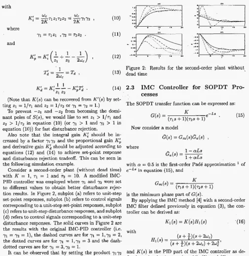
Consider a second-order plant (without dead time) with K = 1, 7 1 = 1 and 72 = 10.
A
modified IMC-P I D controller was employed where 71 and 7 2 were set
to different values to obtain better disturbance rejec- tion results. In Figure 2, subplot {a) refers to unit-step set-point responses, subpIot (b) refers to control signals corresponding to a unit-step set-point responses, subplot (c) refers to unit-step disturbance responses, and subplot (d) refers t o control signals corresponding to a unit-step disturbance responses. The solid curves in Figure
2
arethe results with t h e original IMC-PID controller (i.e. y1 = 72 = l), the dashed curves are for 71= 1,yz = 2, the dotted curves are for y1 = l,y2 = 3 and the dash- dotted curves are for y1 = 3,72 = I.
It can be observed that by setting the product 7172
to be greater than 1, we sacrifice the set-point perfor- mance to secure a faster settling in disturbance rejec- tion. The tradeoff could be achieved over a wide range
of 7 1 ~ 2 , Note that it is more effective to adjust the 7 value that is related to the slow time constant (i.e., 72 in
the above example) to prevent the slow plant pole to be cancelled by the corresponding controller zero. As can be seen in Figure 2, the unit-step set-point response and its corresponding control signal may have been sacrificed
Figure 2: Results for the second-order plant without dead time
2.3
IMC Controller
for
SOPDT
Pro-
cesses
The SOPDT transfer function can be expressed as:
NQW
consider a model( 3 s ) = G - T " a ( s ) I
where
1
-
( Y L Sa 4
=with a = 0.5 is the first-order Pad6 approximation
e - L s in equation (15), and
of .
is the minimum phase part of G ( s ) .
By applying the IMC inethod [4] with a second-order IMC filter defined previously in equation (31, the con- troller can be derived as:
with
(s
+
$)(s -E 2 4and K ( s ) is the PID part of the IMC controIler as de- fined previously via equations (4), (5), and (6).
2.4
Set-point Response
andDisturbance
Rejection Tradeoff for
SOPDT
pro-
cesses
Following the same procedure described in Section 2.2,
disturbance rejection tradeoff for SOPDT processes is found to be:
and.D(s) = (s
+
s ) ( s+
2w,)(s+
$)(s +.$)+
2wz(s+
z1)(s+
22). K'(s] is the modified IMC-PID controllergiven previously via equation (8) with K,l, KA,
Ti,
andKh defined in equations (10),(12),(13), and (14) respec- tively.
Observe that the modified IMC controller for achive- ing set-point response and disturbance rejection tradeoff for SOPDT processes consists of the mudzfied IMC-PID controller for second-order plant without dead time (i.e. K'Is)) cascaded with a fourth order filter H i ( s ) .
3
Tuning
Procedure and Simula-
tions
Before describing a tuning procedure of the IMC con- troller for SOPDT processes, we would make the fol- lowing important observations. Recall that the modi- fied IMC-PID controller for achieving set-point response and disturbance rejection tradeoff €or second-order plant without dead time is defined by three tuning parame- ters [namely, w c , 71 and 7 2 ) . By setting y1 = 7 2 = 1
(corresponding to setting z1 = l / r ~ and 22 = l / r z )
,
we recover the originaI IMC-PID controIler K ( s ) shown in equation (4) from the modified IMC-PID controller
K ' ( s ) shown in equation (9). As shown in equation (16), the original IMC controller for SOPDT process con- sists of the original IMC-PID controller for second-order process without dead time cascaded with a second or- der filter H , ( s ) while, as shown in equation (17), the
mod$ed
IMC
controllerfor achieving
set-point response and disturbance rejection tradeoff for SOPDT processes consists of the modified IMC-PID controller for second- order processes without dead time K ' ( s ) cascaded with a fourth order .filter H i ( s ) . Once we have observedthese
relationships between K'(sj and K ( s ) , K { ( s ) andK1 (s), the tuning procedure of the modified IMC-PID controllers for SOPDT processes can be described as fol- lows:
1. Specify the desired cIosed-loop performance in terms of the designed closed-loop bandwidth w, as if we are going to control the plant by the original IMC controller
K 1
(s).Figure 3: Results for Example 1
2. Set 71 = 7 2 = 1 and apply the value of w, ob- tained from the previous step to the modified
IMC
controller K i ( s ) . That is, initialise the modzfied
IMC
controllerK i ( s )
to give good set-point step response (and possibly slow settling disturbance re- jection).3. If the disturbance rejection is not sufficiently fast, increase the value of the appropriate 7 from 1 to
speed up the disturbance rejection. For processes with real and distinct poles, increase the value of 7 related to the slower time constant. For processes with equal real poles or complex conjugate poles, increase the values of 71 and 'yz equally.
4. Fine tune
K{(s)
by making incremental changes to the values of the appropriate y (and w, if necessary)until the desired results are obtained.
We shall now present some simulation examples. In each of the following figures, subplot (a) refers to unit- step set-point responses, subplot (b) refers to control signals corresponding to a unit-step set-point responses, subplot (c) refers to unit-step disturbance responses, and subpiot (d) refers t o control signaIs corresponding to a unit-step disturbance responses.
Example 1
In this example, a SOPDT plant with T~ t= 1 sec, r2 =
10 sec,
K
= 1, andL
= 1 sec is used. The dominant time constant is 10 sec and the normalised dead time isL / r = 0.1 in this case. We used w c = 0.5 r a d / s . The. results are shown in Figure 3.
The solid curves in Figure 3 are the results with the original IMC controller (corresponding to y1 = 7 2 = 1),
the dashed curves are for y1 = 1, yz = 2 and the dotted curves are for 71' = l,y2 = 3. Observe how we sacri- fice the set-point performance to secure a faster settling disturbance rejection.
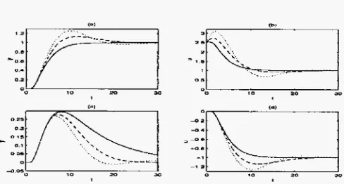
Example 2
In this example, a SOPDT plant with q = 1 sec, ~2 = lOsec, K = 1, and L = 5sec is used. The dominant
Figure 4: Results
Figure 5: Results
for Example 2
<"I
I I
for Example 3
time constant is 10 sec and the normalised dead time is
LIT = 0.5 in this case. We again used we = Q.5 radls. The results are shown in Figure 4.
The solid curves in Figure 4 are the results with the
original IMC controller, the dashed curves are for y1 =
X,y2 = 2 and the dotted curves are for 71 = 1,yz = 3. Observe again that we sacrifice the set-point perfor- mance to secure a faster settling disturbance rejection. Note that the tradeoff achieved with the same values of 71and 72 is more limited in this example than that of
Example 1 due to the higher value of the normalised dead time LIT.
Example 3
In this example, a SOPDT plant with 7 1 = 1 sec, q
=
lOsec, K = 1, and L
=
lOsec is used. The dominant time constant is 10 sec and the normalised dead time isL / r = 1 in this case. We have kept w, at 0.5 radls.' The results are shown in Figure 5.
The solid curves in Figure 5 are the results with the original IMC controller, the dashed curves are for y1 =
l,yz = 2 and the dotted curves are for 71 = 1,yZ = 3. Note that the tradeoff achieved with the same values of
yl and 7 2 is even more limited in this example than that
Figure 6: Results for Example 4
Figure 7: Results €or Example 5
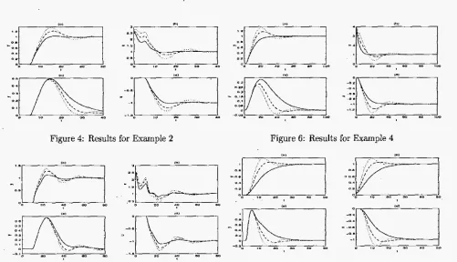
Example
4
In this example, a SOPDT plant with equal time con- s t a n t s is used (i.e., TI = 10sec, TZ = 10sec,
K
= 1,and L = 1 sec). The normalised dead time is L / T = 0.1 in this case. We used U,
=
0.2 r a d / s . The results are shown in Figure 6.The solid curves in Figure 6 are the results with the original IMC controller, the dashed curves are for y1 =
7 2 =
fi
and the dotted curves axe for 71 = ~2 =&.
Note that the tradeoff is achieved with the equal valuesof y1 and TL (since TI = ~ 2 2 ) .
The following examples deal with SOPDT plant with
complex conjugate poles. The SOPDT plant transfer function is in the form of
4
e-L8G(s) = K
$2
+
2Cwns 4- w:where w,, is the undamped natural frequency and
C
is the damping factor of the SOPDT plant.Example 5
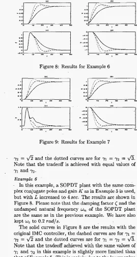
Figure 8: Results for Example 6
Figure 9: Results for Example 7
7 2 =
fi
and the dotted curves are for y1 = 72 =a.
Note that the tradeoff is achieved with equal values of71and 7 2 -
Example 6
. In this example, a SOPDT plant with the same com- plex conjugate poles and gain K as in Example 5 is used, but with
L
increased to 4sec. The results are shown inFigure 8. Please note that the damping factor
C
and the undamped natural frequency un oE the SOPDT plantare the same as in the previous example. We have also kept wc to 0.2 T ~ / . s .
The solid curves in Figure & are the results with the original IMC controller, the dashed curves are for 71 =
yz =
fi
and the dotted curves are for y1 = 7 2 = 6.Note that the tradeoff achieved with
the
same values of 71and 7 2 in this example is slightly more limited than that of Example 5. This is mainly due to the larger value of L in the SOPDT plant.' Example 7
In this example, a SOPDT plant with complex con- jugate poles p l = -0.25
+
0.9682j and pz = -0.25-
0.96823' is used, while K = 1, and L=
2sec. This again corresponding to w, = I r a d / s e c and<
= 0.25. We again used w, = 0.2 r a d l s . The results are shown in Figure 9. Please note that the damping factor of the SOPDT plant in this example is much lower than the one in Example 5.The solid curves in Figure 9 are the results with the original IMC controller, the dashed curves are for 71= .
72 =
&
and the dotted curves are €or y1 = 7 2 =a.
Note that the tradeoff is achieved with equal values of
y1 and 7 2 .
Note that in Examples 1, 2, 3 and 4 only real poles in the
SOPDT
plant have been considered. However, the tuning procedure can be easily extended to SOPDT plant with complex conjugate poles as illustrated in Ex- amples 5 , 6, and 7.From the results of the Examples 1, 2, 3, and 4 we can make the following important observation. The achie- veable tradeoff between set-point response and disturbance rejection for SOPDT processes un- der IMC control is limited by L / T of the pro-
cesses for the simple pole cases, where T is the
dominant time constant of the SOPDT processes. For SOPDT plant with complex conjugate poles, the factor which limits the achieveable tradeoff between set-point response and disturbance rejection under IMC control needs to be examined further in future work.
4
Conclusions
In this paper, we have presented some derivation of IMC controllers and tuning procedures when they are applied to SOPDT processes for achieving set-point re-
sponse and disturbance rejection tradeoff. We have dis- covered that for controllers designed by following the
IMC approach, the integral gain, the proportional gain, the derivative giin plus a fourth-order filter of the con- troller shouId all be adjusted according t o the given for- mulas and tuning procedure presented for the purpose of achieving set-point response and disturbance rejection tradeoff. The study has also shown that the tradeoff Between set-point response and disturbance rejection is again limited by the normalised dead time for the simple pole cases. For SOPDT plant with complex conjugate poles, the factor which limits the achieveable tradeoff b e
tween set-point response and disturbance rejection un- der IMC control needs t o be examined further in future work.
References
[I] W.K. Ho, O.P. Gan, E.B. Tay and E.L. Ang, Per-
formance and Gain and Phase Margin of Well-
Known PILI Tuning formulas, IEEE Trans. Control System Technology, 4 (1996), pp. 473-477.
[2] W.K. Ho, K.W. Lim and W. Xu, Optimum Gain
and Phase Margin Tuning for PID Controllers, Au-
tomatica, 34 (1998), pp. 1009-1014.
[3] W.S. Lee and J. Shi, Modified IMC-PID Con-
trollers and Generalised PID Controllers for First Order Plus Dead Time Processes, Proc. 7th Int. Conf. on Control, Automation, Robotics and Vi-
sion, ICARCV, Singapore, (2002), pp. 898-903.
[4]
M.
Morari and E. Zafiriou, Robust Process Control[5] B.A. Ogunnaike and W.H. Ray, Process Dynamics, Modding, and Control (Oxford University Press, New York, 1994).
(Prentice-Hall, New' Jersey, 1989).
161 J.Shi and W.S.Lee, IMC-PID Controllers for First
Order Plus Dead Time Processes:
A
Sample Design,with Guaranteed Phase Margin, R o c . IEEE Region 10 Tech. Conf. on Computers, Communications, Control and Power Engineering, TENCUN'02, Bei- .. jing,' C l h a , (2002); pp. 1397-1400.
[7] F.G. Shinskey, Process Control Systems: Applica- tion, Design, and Tuning, 3Td edn. (McGraw-Hill, New York, 1988).
[SI Q.G. W m g , C.C. Hang, and X.P. Yang, Single-Loop Contp.oilers Design via IMC Principles, Automat- ica, 37 (20011, pp. 2041-2048.
[9] W.A. Wolovich,~Autom~utac 'Control Systems: 'Basic
Analysis and Design (Saunders, Orlando, 1994).
[la]
S.
Yamamoto and I. Hashimoto, Present Status andFuture Needs: The View from Japanese Industry,
in: Y . Arkun and W.H. Fay, eds., Proc. 4th Ink. Conf. on Chemical Process Control, (AICHE, New York, 1991).
[11]
M.
Zhuang and D.P. Atherton, Automatic Thing of Optimum PID Cont~.olEers, IEE Proceedings-D, 140, (1993), pp. 21&224.11.21 K.J. Astrom, C.C. Hang, P. Persson, and W.K. Ho, Towards Intelligent
PID
Control, Automatica, 28[13] K.J. Astrdm and T. Hagglund,
PID
Controllers: Theory, Design, and Tuning (Instrument Societyof America, New Carolina, 1995).