Natural Continuous Extension Implicit Runge-Kutta Method for Solving Nonlinear DDE in Blood Cell Production

(1)

402

Natural Continuous Extension Implicit Runge-Kutta

Method for Solving Nonlinear DDE in Blood Cell

Production

K.Ponnammal1, R.Sayeelakshmi2,

Department of Mathematics1, Periyar E.V.R. College, Tiruchirappalli-6200231

Department of Mathematics2, Mookambigai College of Engineering, Keeranur, Pudukkottai-6225022 Email: [email protected], [email protected]2

Abstract- Numerous amazing physical phenomena are much of time demonstrated by non-linear Delay Differential Equations (DDE) in the field of Science and Technology. The Mackey–Glass equation illustrates non-linear phenomena in physiological control systems in which the dynamics of the density of blood cells is considered. The Mackey- Glass equation is the representative example of delay induced chaotic behavior. The dynamics of Mackey- Glass equation examined utilizing Natural Continuous Extension (NCE) of Implicit Runge-Kutta method of fourth order with Cubic Spline interpolation used to approximate the delay term. The commitment in this paper focuses with the derivation of coefficients for continuous Implicit Runge-Kutta method for fourth order. This method considers the minimum number of stages than Runge-Kutta Fourth order method. Numerical solution of Mackey -Glass equation simulated for a different delay yielding the periodic and chaotic dynamics.

Keywords- DDE, Runge-Kutta method, Natural Continuous Extension, Cubic interpolation, Mackey-Glass. 1. INTRODUCTION

The Mackey and Glass introduced a first non linear delay differential equation in 1977 to model physiological system as.





m m m

dy k y(t )

y(t)

dx y t

  

  

    (1)

where parameter α , k > γ > 0, m



R+, y(t) signifies the current density of white blood cells, γ represents decay rate.



is the time delay between the production of immature cells in the bone marrow and their maturation for blood stream and the history function y(t)= 0.5 for t<0.

The exact solution of physiological model becomes a difficult task if the equation is highly nonlinear. Such equations are difficult to solve analytically. Researchers utilize the numerical strategies to find out approximate solution to non linear delay differential equation. Motivation behind the Mackey-Glass equation is from a physiological point of view; however the equation has been applied to other disciplines in science and engineering. In this way, the mathematical properties and implementation of the equation are investigated for varying parameters. Mackey-Glass equation affords a objectives for the application of new techniques for non-linear delay differential equations while it can generate varied dynamics, from convergence to oscillations with different characteristics and even chaotic behaviour. Despite intensive research over the decades with the analytical, numerical and even

experimental studies of chaotic behaviour emergence is not satisfied yet.

2. RELATED WORK

Researchers have shown growing interest towards chaos control, and numerous techniques have been proposed. The Mackey-Glass equation was basically created to model blood production and destruction in the study of oscillation and chaos in physiological control systems [12]. It is used to determine the rate of blood production in a person. The equation computes Periodic and chaotic dynamics J.C.Sprott [13] described the simplest chaotic delay differential equation with a sinusoidal non-linearity, including the route to chaos, Iyapunov exponent spectrum, and chaotic diffusion which is prototypical of numerous other high-dimensional chaotic system. Mackey and Foley[10] expressed that the equation display a range of periodic and chaotic dynamics on the value of parameter and its mathematical properties are explored in the biological perspective.

(2)

403 Gopalsamy et al. [11] investigated the global

attractivity for the model Eq. (1), though Ambrosio and Jackiewicz [2] constructed continuous extensions to Runge–Kutta (RK) methods for ordinary differential equations. Baker and Paul [3] discussed about the practical determination of stability regions when various fixed step-size RK methods, joined with continuous extensions, are applied to the linear delay differential equation with fixed delay. The solution for Eq. (1), is approximated by applying reliable, efficient, and more convenient techniques. The paper is structured as follows: Related Work is described in Section 2. Section 3 discusses the ordinary differential equations (ODE) continuous RK method. Section 4 derives NCE for Implicit RK coefficients for DDE. In Section 5, the Cubic Interpolation method used to find a delay term is given. Section 6 represents the solution of Mackey-Glass equation which is followed by the conclusion.

3. CONTINUOUS RK METHOD FOR ODE

Given a mesh





f N n ,t,....t,....t t

t

Δ ₀₁  a v-stage R-K method for the numerical solution of the ODE

 



 



 

0 f

0 0

y t g t, y t , t t t

y t y

    

 

 

(2)

has the form





v

i j j

n 1 n n 1 ij n 1 n 1 j 1

Y y h  a g t , Y , i 1,....v



 





(3)



t Y



, g

b h y

y i_n_1, _ni₁

nu 1 i

i 1 n n 1

n  

 

  



(4)

Where

v

i ij

j 1

c a ,





i= 1,.... v ,

h

_{n 1}_



t

_{n 1}_



t

_n and v

is referred as the number of stages. The bi ’

s are called weights of the quadrature formula and ci

’

s[0,1] are called abscissa. The one - step interpolants of the RK method given in Eq. (3), and Eq.(4) are formed step by step by making use of information from the underlying mesh interval [tn,tn+1] only, possibly by

including some additional stages, that is, by some extra evaluations of the right-hand-side function g(t,y) in Eq. (2). Interpolants derived using no extra stages are called interpolants of the first class. The value obtained from continuous extension 

 

t is defined in each sub interval of the mesh



,

by a one-step continuous quadrature rule of the form





v

 





i i n n 1 n n 1 i n 1 n 1

i 1

η t θh  y h b θ g t ,y  0 θ 1



  



  (5)

(or) in the K- Notation





v

 

i

n n 1 n n 1 i n 1 i 1

η t θh  y h  b θ K  0 θ 1



  



  (6)

where theb_i

 

θs are polynomials of suitable degree



 satisfying

bi (0) = 0 and bi(1) = bi, i = 1,...v (7)

So as to satisfy the continuity conditions 

 

tn ynand

 

tn 1 yn 1

 

(8)

4. CONTINUOUS EXTENSION OF RK

METHODS FOR DDE

The first order delay differential equation has the form

 



 



 



   

0 f

0

y t f t, y t , y t t, y t , t t t

y t t , t t

      

 

  

 (9)

The standard method for solving the DDE, consists in solving step by step the local problems

 



 



 



 

n 1 n 1 n 1 n n 1

n 1 n n

t f t, t , x t t, t , t t t

t y

   



        

 

 



(10)

where

 

0

0 n

n 1 n n 1

s for s t

x(s) s for t s t

s for t s t

 

 



   

  



(11)

and 

 

s is the continuous approximate solution computed up to tn.

The overall method for DDE is presented as













v i

n 1 n n 1 ij

i 1

j j j j j

n 1, n 1 n 1 n 1 n 1

Y y h a

f t Y ,η t τ t ,Y , i 1,...s

 



    

 

 



(12)

   













v

n n 1 n n 1 i

i 1

j j i i i

n 1, n 1 n 1 n 1 n 1

η t θh y h b θ

f t Y ,η t τ t ,Y , 0 θ 1

 



    

  

  



(13)

The Eq. (12) and Eq. (13) are called the RK method for DDE. The coefficients (A, b) are the underlying discrete RK method, whereas (A, b (θ)) are the interpolants. The pair formed by the underlying discrete RK method and interpolants is called the underlying continuous RK method.

In the mesh interval [tn, tn+1], the Eq. (12) and Eq. (13)

takes the form





 





v

n n 1 n n 1 i

i 1

i i i

n 1, n 1 n 1

η t θh y h b θ

f t Y ,:Y , 0 θ 1

 



  

  

 



(14)





v

i j j j

n 1 n n 1 ij n 1, n 1 n 1

i 1

Y y h a f t Y ,Y ,

i 1,...v

    



 





(15)

where the spurious stages yni1are given by

  



v

i i j j j

n 1 n n 1 j n 1 n 1, n 1 n 1 i 1

Y_ y h_ b θ_ f t Y ,Y_ _ _ ,



 



(3)

404 If

t

i_n_₁



τ



t

_ni_₁

,Y

_ni_₁



,



t

_n and by







i



1 n i 1 n i 1 n i 1

n ηt τt ,Y

Y      (17)

Otherwise, the system Eq. (14), Eq. (15) and Eq. (17) has to be solved only for the stage values, j

n y 1, j =

1…v, the system enlarged by Eq. (16) for some it has to be solved also for the relevant spurious stage value

i

n 1

y  .

5. NCE FOR IMPLICIT RK METHOD

Zennaro [14] developed the NCE of first class interpolants of RK method. The interpolant 

 

t in (4) of order p is a NCE of the RK method (3) of degree q if the polynomials, b_i

 

 i=1, 2...v are such that

 

t

 satisfies the additional asymptotic orthogonality condition as

     

 

1

1     



 p

t t h O dt t η t y t G n n (18)

For every sufficient smooth matrix valued function G and with the statements 

 

t₀ y ,₀ 



t₀h



y₁

hold.

The RK method is accurate of order p (1) satisfies





 

1

0      p h O y h t y .

The approximate solution find iteratively on a mesh ∆={t0,t1,t2…tn….tN=tf} of the interval (t0,tf), such that

 

0 0 h

q

t t t

y t t O h

max



     

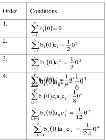
[image:3.595.304.510.515.770.2]

(19) Table 1. Order condition for Continuous RK

method.

Order Conditions

1.

 

θ θ b v 1 i i 





2. _{ } 2

i v 1 i i θ 2 1 c θ b 





3.

 

2 2

i v 1 i i θ 3 1 c θ b 





 

3

j ij v 1 i i

θ

6

1

c

a

θ

b







4. v

 

3 4

i i

i 1

1

b θ c θ

4  



 

v 4 i i ij j i,j 1

1

b c a c θ

8



 



 

2 2

j ij v 1 j i, i θ 12 1 c a θ b 





 

4

k ij v 1 k j, i, i θ 24 1 c a θ b 





It is to be noticed that the collocation polynomial for

any one-step collocation method is as NCE of degree q = v. The theorems 4.1 to 4.3 are given by Zennaro [14].

Theorem: 5.1

Every RK process Eq.(4) and Eq.(6) of order p has a NCE 

 

t of minimal degree

      2 1 p q . Theorem: 5.2

If the interpolant Eq. (5) of order (and degree) q is an NCE of the RK method Eq.(4) and Eq. (5) of order p, then       2 1 p q . Theorem: 5.3

Every Runge-Kutta method of Eq. (2) of order p1 has a continuous extensionη

 

t of order q=1 ...

     2 1 p . The polynomial b_i

 

 satisfies the condition

 

i

b 0 0 and

 

r

i c b dθ θ b

θ i i

1 0

r  _



r = 0,...q . (20) The NCE of RK method is not unique and Eq.(20) provides a rule for obtaining one of them. The Table.1 and Table.2 are given by Butcher [6],[7]. The order condition stated in Table.1 is used to obtain the NCE of RK method. Table.2 represents the coefficient tableau for NCE four stage IRK of order p=4, c1= 0, [image:3.595.97.269.516.743.2]

c2 ≠ c3, c4 = 1 and distinct,34



c₂c₃



6c₂c₃0

Table 2. RK Coefficient Tableau. 0

c2 c2

c3







2



2 2 2 3 2 3 2 1 2 4 3 c c c c c c   









1 3 2

2 2

c c c 2c 1 2c

 

1 a41 a42 a43

b1 b2 b3 b4

where



 









2 3 2 3



3 2 2 2 2 2 2 2 3 2 2 2 2 3 41 c 6c c c 4 3 c 2c 2 6c 4c 5 15c 12c c 4 12c 12c c             a











3 2







2 3



2 3



2 2 2 3 2 3 42 c 6c c c 4 3 c c 2c c 1 2 c 5c 4c a          









3 2







2 3



2 3



3 2 3 2 43 c 6c c c 4 3 c c c c 1 c 1 2c 1 a        





3 2 3 2 3 2 1 c 12c c 6c c c 2 1

b    



3 2



2



(4)

405





2



2 3 2 3

b₃ 1 2c

12c c c 1 c

 

 







2 2



3 32 3



b₄ 3 4 c c 6c c 12 1 c 1 c

  



 

From theorem 4.1 it follows that NCE of minimal degree       2 1 p

q = 2 for p=4,

The second degree polynomial stated as

 

θ ξθ ηθ

b i

2 i

i   where ηibiξi, i = 1,2,3,4 (21) satisfies the order condition from Table 1 up to order 2, Then the equations used are given as,

 

θ θ

b v 1 i i 





and (22)

 

2

i v 1 i i θ 2 1 c θ b 



 (23)

Putting i = 1,2,3,4 in equation (20) we get

 

2





1 1 1 1 θ

b θ ξ θ  b ξ (24)

 

θ ξθ



b ξ



θ

b 2 2

2 2

2    (25)

 

θ ξ θ



b ξ



θ

b 2 ₃ ₃

3

3    (26)

 

2





4 4 4 4

b θ ξ θ  b ξ θ ₍₂₇₎ From Eq. (22) and Eq. (23), we arrive at

 

1 2 3 4

b θ b θ b θ b θ 

 

1 2

b θ c b θ c b θ c b θ c θ

1 1 2 2 3 3 4 4₂

To find b4

 

θ :

 

2

 

4 4 2 2 3 3

1

b c b c b c

2

      

(28)

Substituting Eq. (25) and Eq. (26) in Eq. (28) we get,

2 2 2

2 2 2 2 2 2 3 3 3 3 3 3

1 θ ξ c θ b c θ ξ c θ ξ c θ b c θ ξ c θ 2

      

ξ c

ξ c b c ξ c

1 ₂ _{2 2} ₂ _{2 2} _{2 2} _{3 3} ₂

θ θ θ θ θ

2c c c c c

4 4 4 4 4

b c ξ c

3 3_θ 3 3_θ

c c 4 4        2 3 3

2 2 2 2 2 2

4 4 4 4 4

3 3 3 3

4 4

ξ c

ξ c b c ξ c

1

θ θ θ

2c c c c c

b c ξ c

- θ θ

c c

 

_   _  

 



Substitute 2 4

c



  3

4

c



  in the above equation

2

4 3 3 3

4 2 2 2 4 2

4 4 4 4 4 4

4 3

4

c μc b c

c λc b c c λc

1 _θ _θ _θ- _θ+

2c c c c c c

c μc θ c          

2 2 2 3 3

2 3 2 3

4 4 4

b c b c

1

λc μc θ θ λc θ θ+μc θ

2c c c

 

_   _   

 





2

2 3 2 2 3 3 2 3

4 4

1 θ

λc μc θ b c b c λc θ c θ

2c c   _   _       





2

2 3 2 2 3 3 2 3

4 4

1 θ

λc μc θ b c b c λc θ μc θ

2c c

 

_   _    

 

2

2 3 4 4 2 3

4 4

1 θ 1

λc μc θ b c λc θ μc θ

2c c 2

   

_   _  _  _ 

 

2 4 4

2 3 2 3

4 4 4

b c θ

1 θ

λc μc θ λc θ μc θ

2c 2c c

 

_   _    

 

2

2 3 4 2 3

4 4

1 θ

λc μc θ b θ λc θ μc θ

2c 2c

 

_   _    

 

Hence,

 

2

4 2 3 4 2 3

4 4

1 1

b λc μc θ b θ θ λc μc

2c 2c

   

 _   _   _   _

    (29)

To find b₃

 

θ :

 

2

 

2 4

 

4

2 3

3 θ b θ c b θ c

2 1 c θ

b    (30)

Substituting Eq. (25) and Eq. (29) in Eq. (30) we get,

 

b

 

θ

c

θ

b

c

θ

2c

1

θ

b

₄ 3 4 2 3 2 2 3

3









2 2 3

2 2 2 4 4

2 2 2

3 3 3

4 2 3

4

1

λc μc θ

c c

1 2c

θ ξ θ b ξ θ

1

2c c c

b θ θ λc μc

2c                 _   _       _   _      





2 2 3 4

2 2 2 4

4 2 4

3 3 3

4 2 3

4 1 c c 2c c c 1

c b c

2c c c ₁

b c c

2c                   _      _ _ _   _{  }_ _{  } _  _ _   

2 2 2 2

2 2 4 2 2 2 4 4 2 4

3 3 3 3 3 4 3

2

3 4 4 4 4 2 4 3 4

3 3 3 4 3 3

c c λθ c b θ c c λθ c θ c c λθ 1 θ

2c c c c 2c c c

c c μθ b c c θ c c λθ c c μθ

c c 2c c c c





    

    

2

2 2 4 4

4 4

3 3 3

c b θ b c θ θ

c μθ c μθ

c c 2c

     





2

2 2 4 4 4 4

3 3

θ θ

c b b c c μθ c μ

c 2c

      

2

4 4 3 3

3 3

θ θ 1

c μθ c μθ b c

2c c 2

 

    _  _

 

2 3 3

4 4

3 3 3

b c θ

θ θ

c μθ c μθ

2c 2c c

(5)

406 Hence,

 

2

3 4 4 3

b       c c b (31) To findb₂

 

 :

 

2

 

2 2 3 3 4 4

1

b c b c b c

2

      

(32) Substituting Eq. (31) and Eq. (29) in Eq. (30) we get

2 2 3

2 2 4

3 4 4 3 4

4 2 3

4

1

λc μc θ

1 2c

θ c c μθ c μθ b θ c

1 2

b θ θ λc μc

2c

  

 

  

 

 

 

  _   _

 

 

  _   _

 

 

 

2 3 2

4 4 3

2 2

2 4

2 3 4 2 3

2 4 4

c

1 θ c μθ c μθ b θ

2c c

c 1 1

λc μc θ b θ θ λc μc

c 2c 2c

 

  _   _

 _ _  _ _  _ _ 

   

   

 

2 2 2

2 3 4 4 3 3 3 4 2 4

2 2 2 2 4 2 2

2

3 4 4 4 4 2 4 3 4

2 2 4 2 2 2

c c μθ c μθc b θc c θ λc c θ

1 θ

2c c c c 2c c c

μc c θ b θc θc λc θc μc θc

c c 2c c c c

     

    

2

3 3 4 4

4 4

2 2 2

b θc b θc θ

λc θ λθc

c c 2c

     





2

3 3 4 4 4 4

2 2

θ θ

b c b c λc θ λθc

c 2c

     

2

2 2 4 4

2 2

θ 1 θ

b c λc θ λθc

c 2 2c

 

  _  _  

 

2

2 2

4 4

2 2 2

b c θ

θ θ

λc θ λθc

2c c 2c

     

Therefore,

 

2

2 2 4 4

b  b      c c (33) To findb₁

 

 :

 

1 2 3 4

b    b  b  b 

(

34

)

Substituting

b

2

   



, b

3



& b

4

 



in Eq. (34) we

get

2

2 4 4

2

2 3

2 4

4 4 3

4 2 3

4

θ b θ λc θ λθc 1

λc μc θ 2c

c μθ c μθ b θ

1

b θ θ λc μc

2c

 

 _   _

  

 

  

 

 

   

  _ _ __

  _   _

 

 

 

2 2

4 2 4 4 4

2

2 2

3 2 3 4 2 3

4 4

θ λc θ b θ λc θ c μθ μc θ

θ θ

b θ λc θ μc θ b θ λc θ μc θ

2c 2c

     

       





2

2 3 4 4 4 2 3

4

4 4 2 3

4

1

θ 1 b b b θ λc c μ λc μc

2c 1

θ λc μc λc μc

2c

 

     _     _

 

 

 _     _

 

 

















2

1 1 4 2 4 3

4

4 2 4 3

4

1

b θ b θ θ λ c c μ c c

2c 1

θ λ c c μ c c

2c

  

  _     _

 

  

 _     _

 

For the finding the NCEs of order q=2, put r = 1 in

 

i i

1 0

i θdθ b c b

θ  







i i i

ξ 3b 2c 1

We know that

 

 2







i

i i

b   b  





2





i i i i i

3b 2c 1 θ b 3b 2c 1 θ

    





2





i i i i i i

3b 2c 1 θ b 6b c 3b θ

    

 

θ 3b



2c 1



θ



4b 6bc



θ

b i i i

2 i i

i    

and therefore,

 





2





i i i i i

b θ =3b 2c -1 θ +2b 2-3c θ

(35)

where





3 4 2

b c

1 2c 3

λ 

,





3 4 3

b c

1 2c 3

μ  

Table 3 gives the coefficient of Implicit RK fourth order method [8].

Table 3. Implicit RK fourth order method coefficients.

0 0

1/3 1/3 2/3 -1/3 1

1 1 -1 1

1/6 3/8 3/8 1/8 From Table 3, Eq. (31) becomes

 

θ

2 1 θ 8

3 θ

b₁   2

  θ

4 3 θ 8

3 θ

b 2

2 

 

 

2

3 θ

8 3 θ

b 

 

θ

4 1 θ 8

3 θ

b₄   2

6. Cubic Spline Interpolation Method

Definition : Suppose that





x

k

,

y

k





n_k0 are n+1 points, where

a



x

₀



x

₁







x

_n



b

.

The function S (x) is called a cubic spline [9] if there exists n cubic polynomials Sk (x) with coefficients Sk,0, Sk,1,

Sk,2 and Sk,3 that satisfy the properties:

 ( ) ( ) ( )2 ( )3

,0 , ,2

)

,3 (

1

S x S S x x S x x S x x

k k k k

x S

k

    

    

(6)

407

 S x( _k)y_k for k=0,1,...,n-1. The spline passes through each data point.

 S_k_₁(x_k_₁)S_k_₁(x_k_₁)for k = 0,1, .... , n-2. The spline forms a continuous function over [a,b].

 ' '

1 1 1

( ) ( )

K k k k

S x _ S _ x_ for k = 0,1, ... , n-2. The spline forms a smooth function.

 '' ''

1 1 1

( ) ( )

K k k k

S x _ S_ x _ for k = 0,1, ... , n-2. The second derivative is continuous.

7. Numerical Results:

Numerical investigation of Eq.1 on [0,200] with history y(t)=0.5 for t0 is done. The proposed method has been implemented by adapting this problem to the NCE of implicit RK method of fourth order. The delay term is unknown and has to be determined from the cubic spline interpolation. A numerical solution is arrived for this proposed work using Matlab. Depending on the values of the parameters, this equation displays a range of periodic and chaotic dynamics. The dynamics of the density of blood cells is increasingly complex as the delay grows. When there is no delay,



= 0, there is a stable equilibrium point which becomes unstable with increasing delay and different periodic solutions appear. The behavior of the solution y(t) for the case b=2,α=1,γ=1and m=20 for different delay =0,1,2,5,6 and 8 is depicted in Figure.1 to Figure 4. The equation exhibits periodic characteristics of the delay differential equation. For certain values of parameters, this model gives chaotic solution. In practice, chaotic solutions represent Leukemia disease. Mackey –Glass equation was used to model the rate of change of density of white blood cell. The numerical simulation of Eq.(1) indicate that if the delay is Zero then there is a oscillation(Fig.1). When the delay is increased the numerical simulations gives rise to periodic solution. When the delay is further increased, it is observed that



lies between 2 and 5 the dynamics of equation depicted in Fig.2-4. There is a aperiodic chaotic pattern observed for



5.

Fig.1. The dynamics of Mackey Glass Model with k=2,



=1, 1,tau=0,m=10.



=1,  1, tau=1,m=10



=1,  1

,

tau=2, m=10

Fig.4. The dynamics of Mackey Glass Model with k=2



=1, 1

,

tau=5,m=10



=1,  1

,

tau=6,m=10



=1,  1

,

tau=8,m=10

Conclusion

This paper develops the theory of Natural Continuous Extensions (NCEs) for the discrete approximate solution of an ODE given by a Runge-Kutta process. These NCEs are defined in such a way that the

0 20 40 60 80 100 120 140 160 180 200 0.5

0.6 0.7 0.8 0.9 1

t

x

(t

)

0 20 40 60 80 100 120 140 160 180 200

0 0.5 1 1.5

t

x

(t

)

0 20 40 60 80 100 120 140 160 180 200 0

0.5 1 1.5 2

t

x

(

t

)

0 20 40 60 80 100 120 140 160 180 200 0

0.5 1 1.5

t

x(

t

)

0 20 40 60 80 100 120 140 160 180 200 0

0.5 1 1.5

t

x(

t

)

0 20 40 60 80 100 120 140 160 180 200 0

0.5 1 1.5

t

x(

t)

1.6

(7)

408 continuous solutions furnished by the one-step

collocation methods are included.

The dynamic behavior of a first order delay Mackey-Glass equation is investigated after applying a NCE implicit RK method of fourth order with 2 stages along with cubic spline interpolation to approximate the delay term. Figures1-6 gives the solution for various parameters. It can be concluded that the mathematical model with the NCE of RK approach is considered appropriate in accommodating the inadequacy of solving the numerical solution to the Mackey Glass equation model.

REFERENCES

[1] O.S Adesina, O.K Famurewa, and R. J Dara, O.O Agbool,a, and O.A Odetunmibi, “The Mackey– Glass type Delay differential equation with uniformly Generated constants”. International journal of mechanical Engineering and Technology Volume 9 , Pages 467-477, 2018. [2] R.D Ambrosio, and, Z Jackiewicz “Continuous

two-step Runge-kutta methods for ordinary differential equations”, Springer Numerical Algorithms Volume 54, Pages 169-193, 2010. [3] C.T.H Baker, and C.A.H Paul, “Computing

Stability regions Runge –Kutta methods for delay differential equation” IMA Journal of Numerical Analysis,Volume14, Pages.347-362, July 1994. [4] A.Bellen, and M.Zennaro, “Numerical Methods

For Delay Differential Equations Clarendon Press”, Oxford, ISBN13: 9780198506546, 2003 [5] A. Bellen, and M. Zennaro, “Numerical solution

of delay equations by uniform corrections to an Implicit Runge- Kutta method”. Numerische Mathematik, Volume 47, Pages.301-316, 1985. [6] J.C Butcher, “Numerical Method for Ordinary

Differential Equations”. Wiley, London, ISBN:978-1-119-12150-3. 2008.

[7] J.C Butcher, “Coefficients for the study of Runge-Kutta integration processes”. Journal of the Australian Mathematical Society, Volume 3, Page 185- 201, 1963.

[8] J.C Butcher, “Implicit Runge-Kutta processes”. Mathematics of Computation, Volume 18, Page 50-64,1964.

[9] M.K.Jain, and S.R.K. Iyengar, “Numerical Methods for Scientific and Engineering Computation”, New Age International Publishers, New Delhi, 2007.

[10] C.Foley, and M.C Mackey, “Dynamic hematological disease a review”, Journal of Mathematical Biology, Volume 58, Page 285-322, 2009.

[11] K. Gopalsamy, S.I Trofimchuk, N.k Bantsur, “A note on global attractivity in model of

hematopoiesis”, Ukraninian Mathematical Journal, Volume 50, Pages 3-12, 1998.

[12] M.C. Mackey, L. Glass, “Oscillation an Chaos in physiological control System”, Science, New Series, Volume 197, Pages 287-289, 1977. [13] J.C Sprott, “A Simple chaotic delay differential

equation”. Physics Letters A , Volume 366 , Pages 397-402. 2007.