Turbulent Boundary Layer
Thesis by
Jonathan P. Morgan
In Partial Fulfillment of the Requirements for the Degree of
Doctorate Of Philosophy in Aeronautics
CALIFORNIA INSTITUTE OF TECHNOLOGY Pasadena, California
2019
c
2019
Jonathan P. Morgan ORCID: 0000-0003-2898-4868
ACKNOWLEDGEMENTS
Many, many people have helped and encouraged me on this very long journey to-wards completing my PhD, none more so than my advisor, Beverley McKeon. She has my eternal gratitude for the guidance and support she provided me through the years, which have been invaluable to my development as a researcher. I would also like to thank Dale Pullin, Tim Colonius, and Dan Meiron for agreeing to serve on my committee.
My research group at Caltech has been the best working environment of my life, thanks to the many wonderful people who have shared it with me. Reeve Dunne, Subrahmanyam Duvvuri, Esteban Hufstedler, Kevin Rosenberg, Tess Saxton-Fox, David Huynh, Sean Symon, Simon Toedtli, Ryan McMullen, Maysam Shamai, Morgan Hooper, Ben Barthel, Mitul Luhar, Rashad Moarref, Scott Dawson, An-geliki Laskari, Arslan Ahmed, and Jane Bae have all helped me with research, helped me laugh, and helped me stay sane, and I am so thankful to each of them. The group’s administrative assistants, Jamie Meighen-Sei and Denise Ruiz, have also been a tremendous resource in supporting both my research and good spirits. I could not have completed this thesis without all of these group members.
I would also like to thank Petros Arakelian, who performed the 3D printing of the roughness surfaces shown in this thesis. His advice and support was essential for designing my experiments.
My first year at Caltech was supported by the Ikawa Fellowship in Aeronautics, gen-erously funded by GALCIT alumnus Hideo Ikawa, to whom I am eternally grateful.
ABSTRACT
PUBLISHED CONTENT AND CONTRIBUTIONS
J Morgan and B McKeon. Relation between a singly-periodic roughness geometry and spatio-temporal turbulence characteristics.Int. J. of Heat and Fluid Flow, 71:322-333, 2018. DOI: 10.1016/j.ijheatfluidflow.2018.04.005.
LIST OF ILLUSTRATIONS
Number Page
2.1 Representation of nonlinear interactions between triadically consis-tent velocity modes, (a) for the canonical case, wherek1,k2,m1,m2, ω1, ω2 ,
0, (b) for the case of periodic roughness, where direct interactions give rise to a stationary response, for example the interactions of the velocity response at roughness wavenumbers (kr,0,0) and (0,mr,0)
giving rise to a response at (kr,mr,0), and (c) again for periodic
roughness, for the case of a static mode and a spatio-temporally vary-ing one givvary-ing rise to a response at a spatio-temporally varyvary-ingK. . . 17 2.2 R1M roughness geometry and measurement locations. . . 31 2.3 R2M roughness geometry and measurement locations . . . 32 2.4 R1M traverse hot-wire probe setup. The pressure probe “A” is used
for hot-wire calibration in the freestream. The hot-wire probe holder “B” holds a hot-wire probe (not shown). Linear stages “C” and “D” allow for streamwise and spanwise adjustment of the hot-wire probe. The post “E” extends below the roughness surface and is mounted to a powered traverse that allows wall-normal adjustment during the experiment. . . 33 2.5 R2M traverse hot-wire probe setup. The pressure probe “A” is used
for hot-wire calibration in the freestream. The hot-wire probe holder “B” holds a hot-wire probe (not shown). The collar “C” holds the probe holder in place with a set screw, allowing streamwise adjust-ment. It is mounted on rod “D” with another set screw, allowing for spanwise adjustment of the hot-wire probe. The post “E” extends below the roughness surface and is mounted to a powered traverse that allows wall-normal adjustment during the experiment. . . 33 3.1 Spatio-temporally averaged (a) velocity profile and (b) velocity deficit
profile for smooth and rough wall geometries, as defined in Section 2.3. . . 38 3.2 Spatio-temporally averaged velocity variance of rough and smooth
3.3 Spatial representations for the R1M case of (a) the mean velocity field ¯u+(x,y,z) on thez=0 plane, (b)the spatial variation in the mean velocity field ˜¯u+(x,y,z) on thez = 0 plane. Red contours indicate a region in which the flow is faster than at other points at the same
y-location. Measurement locations atx/λx=0,0.125,0.25,0.5,0.625,0.75,0.875
are marked with a dashed line. . . 41 3.4 Spatial representations for the R2M case of (a) the mean velocity
field ¯u+(x,y,z) on thez=0 plane, (b)the spatial variation in the mean velocity field ˜¯u+(x,y,z) on thez = 0 plane. Red contours indicate a region in which the flow is faster than at other points at the same y-location. Measurement locations atx/λx=0.25,0.5,0.75,1 are marked
with a dashed line. . . 42 3.5 Spatial representations for the R1M case of (a) the stationary
veloc-ity Fourier mode ˆu+(y;kr,mr,0), (b) the stationary velocity Fourier
mode ˆu+(y,2kr,2mr,0), (c) the stationary velocity Fourier mode ˆu+(y,2kr,0,0),
and (d) the stationary velocity Fourier mode ˆu+(y,0,2mr,0). Red
contours indicate a region in which the flow is faster than at other points at the same y-location. . . 45 3.6 Spatial representations for the R2M case of (a) the mean velocity
spatial Fourier mode ˆu+(y;kx,0,0), (b) the mean velocity spatial Fourier
mode ˆu+(y,0,kz,0), and (c) the mean velocity spatial Fourier mode
ˆ
u+(y,kx,kz,0). Red contours indicate a region in which the flow is
faster than at other points at the same y-location. . . 48 3.7 Comparison of spatially-averaged premultiplied angular frequency
power spectrahωΦ(y, ω)ifor (a) the smooth-wall case, (b) the R1M case and (c) the R2M case . . . 50 3.8 Magnitude of the R1M scale modulation|ωbΦ+(y, ω;k,m)|for (k,m)=
(a)(kr,mr) (b)(2kr,2mr) (c)(2kr,0),(d)(0,2mr). . . 52
3.9 Magnitude of the R2M scale modulation|ωbΦ+(y, ω;k,m)|for (k,m)=
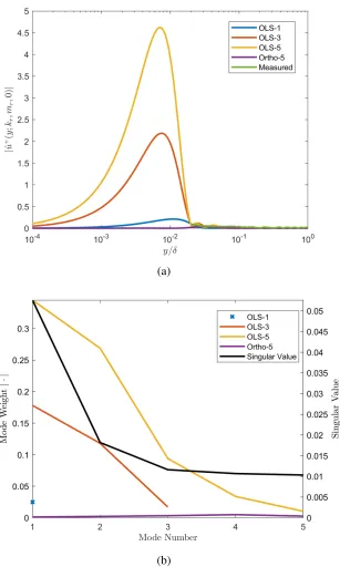
4.1 R1M roughness, (k,m) =(kr,mr) a) Amplitude of measured
station-ary velocity Fourier mode ˆu(green), least-squares fit of the measured velocity to the most-amplified 1 (blue), 3 (red), or 5 (yellow) resol-vent response modes. b)Amplitude of weighting vector entries, same colors as above, plotted on the left y-axis, as well as the singular values for the corresponding resolvent modes, plotted on the right y-axis. . . 59 4.2 R1M roughness, (k,m) = (2kr,2mr) a) Amplitude of measured
sta-tionary velocity Fourier mode ˆu(green), least-squares fit of the mea-sured velocity to the most-amplified 1 (blue), 3 (red), or 5 (yellow) resolvent response modes. b)Amplitude of weighting vector entries, same colors as above, plotted on the left y-axis, as well as the singu-lar values for the corresponding resolvent modes, plotted on the right y-axis. . . 61 4.3 R1M roughness, (k,m)= (2kr,0) a) Amplitude of measured
station-ary velocity Fourier mode ˆu(green), least-squares fit of the measured velocity to the most-amplified 1 (blue), 3 (red), or 5 (yellow) resol-vent response modes. b)Amplitude of weighting vector entries, same colors as above, plotted on the left y-axis, as well as the singular values for the corresponding resolvent modes, plotted on the right y-axis. . . 62 4.4 R2M roughness, (k,m) = (0,2mr) a) Amplitude of measured
sta-tionary velocity Fourier mode ˆu(green), least-squares fit of the mea-sured velocity to the most-amplified 1 (blue), 3 (red), or 5 (yellow) resolvent response modes. b)Amplitude of weighting vector entries, same colors as above, plotted on the left y-axis, as well as the singu-lar values for the corresponding resolvent modes, plotted on the right y-axis. . . 63 4.5 R2M roughness, (k,m)=(kr,0) a) Amplitude of measured stationary
dif-5.7 a)Magnitude of the R2M scale modulation|ωdΦ +
(y, ω;kr,0)|b)Predicted
Scale Modulationζ(y, ω;kr,0). . . 99
5.8 a)Magnitude of the R2M scale modulation|ωdΦ +
(y, ω; 0,mr)|b)Predicted
Scale Modulationζ(y, ω; 0,mr). . . 101
5.9 a)Magnitude of the R2M scale modulation|ωdΦ +
(y, ω;kr,mr)|b)Predicted
LIST OF TABLES
Number Page
C h a p t e r 1
INTRODUCTION
Turbulent boundary layers are a pervasive phenomenon in the fields of climate, in-dustry, and aviation. In many cases of practical interest, the surfaces over which the boundary layers develop are not smooth, and this roughness can alter the important characteristics of the boundary layer, including drag. The study of rough-wall-bounded turbulence must encompass not only the enormous phase space brought on by the expanse of scales in turbulence, but also an incredibly broad parameter space, which includes any surface formed by nature or devised by the human brain. Due to the infinite possible geometric variety of rough surfaces, it is impossible for simulations and experiments to fully explore and document the entire phase space of roughness. This poses a problem for design engineers and analysts who would like to know the effects of a particular arbitrary roughness without perform-ing a potentially costly experiment or simulation, but it also presents an opportunity for scientists. A rough wall can be a slight perturbation to an otherwise-canonical flow. Subjecting the “black box” of canonical wall-bounded turbulence to a slight change and observing the outcome can help expose its inner workings. As outlined in the final section of this chapter, this thesis will connect the study of rough- and smooth-wall flows by creating a simple roughness, documenting its direct linear and indirect non-linear effects on a boundary layer, and creating a simple, cheap, low-order model to explain the observed results.
1.1 The Turbulent Boundary Layer
part of the dominant balance in the equation. Prandtl’s theory divides the flow into two regions: a freestream away from the wall without significant viscous stresses, and a “boundary layer” just above the wall, where viscosity cannot be ignored.
For sufficiently low Reynolds number, a canonical ZPGBL will be steady and lami-nar [9]. For this case, Blasius [8] found a self-similar solution of the Navier-Stokes equations, in which the velocity field is a function only of the freestream velocity and the similarity coordinate χ = y√U∞/νx. A laminar ZPGBL which is
impul-sively perturbed will eventually return to a Blasius profile, with a spatial evolution that has been shifted in x. For this reason, from here, we will take the length scale of a boundary layer to be the 99% boundary layer thicknessδ, the distance from the wall at which the mean velocity recovers to 99% of its freestream value. We will also use a different velocity scale in the friction velocityuτ= pτw/ρ, derived from
the shear stress at the wall τw, for ease of comparison to rough wall flows. The
resulting Reynolds number Reτ = uτδ/ν is called the Karman number or friction Reynolds number. For the ZPGBL, it is bijective and monotonic with other defi-nitions of the Reynolds number, uniquely identifying a flow condition. Quantities normalized byuτare denoted with a superscript plus.
1.2 Similarity and Modeling of Rough-Wall Turbulent Boundary Layers
In addition to the Reynolds number, the characteristics of a rough-wall boundary layer depend on the infinite number of geometrical parameters which describe the surface roughness. Although each individual pattern of roughness presents a unique physical and mathematical case, some patterns emerge across a wide variety of ge-ometries. As in the smooth-wall case, many rough-wall flow quantities scale with the friction velocity uτ and kinematic viscosity ν, and quantities which are non-dimensionalized by these inner variables are denoted with a superscript plus. Flows without sufficient scale separation between the roughness heightkand the boundary layer thickness δ are characterized as “obstacle flows” and have significant quali-tative differences in measured flow quantities throughout the boundary layer when compared to smooth wall flows, including the elimination of the logarithmic layer [32]. Jimenez gives a criterion ofδ/k <40 to separate obstacle flows from
rough-wall flows, which do exhibit some similarity to canonical smooth-rough-wall flows.
inner-normalized streamwise mean velocity u+ scales logarithmically with wall-normal distancey+. Compared to smooth walls, however, the virtual origin of the velocity profile is displaced from the wall and the velocity profile in the logarithmic region is shifted toward slower velocities. The magnitude of this shift is named the “Hama roughness function” and is labeled ∆U+. Subsequent research [48], including by Colebrook [14] with industrial roughness, found that the mean profile of a wide variety of roughnesses can be parameterized in the “fully rough” regime (k+ → ∞) with an “equivalent sand roughness”ks∞. The equivalent sand roughness
of a rough wall is the magnitude of the roughness in Nikuradse’s experiments which would match the∆U+ of that rough wall at highk+. Therefore, the behavior of a rough wall in the fully rough regime is described by a single parameter, though at present no work has provided a general relation between an arbitrary roughness geometry and its equivalent sand roughness [32]. Outside the fully rough regime, with intermediatek+s∞, bothks∞and the roughness geometry figure into the observed
variables, even at very high Reynolds numbers [1]. Between the surface and the logarithmic layer is a roughness sublayer which is believed to extend to several times the sand grain roughness [60].
Wall flows with three-dimensional roughness and sufficient scale separationδ/k ex-hibit similarity with smooth-wall flows beyond just the logarithmic mean profile. Townsend’s hypothesis [69] posits that the boundary layer physics outside of the roughness sublayer are affected by the roughness only through the length and ve-locity boundary conditions which the sublayer imposes on the rest of the flow. In this description, the roughness elements serve only to perturb the turbulent cascade in the roughness sublayer, altering the velocity profile near the wall and therefore the wall shear stress. The resulting values ofuτandδthen provide the scales for the flow statistics in the outer layer, so that rough-wall quantities of the form Q+(y/δ)
are identical to smooth-wall quantities at the same Reynolds number. Schultz and Flack [65] find such a similarity for the velocity defect U∞+ − U+ and for
single-point velocity correlations up to third order. Flores et al. [21] provides evidence for this view, observing roughness-like similarity in simulated flows with prescribed velocities and Reynolds stresses at the wall.
rough-ness. Using experimental data up to high Reynolds number (Reτ ≈2800−17400), Morrill-Winter et al., [49] find a dependence of normalized wall-normal velocity variance on roughness conditions in the wake region of a sandpaper-roughness boundary layer, well outside the roughness layer. Mejia-Alvarez and Christensen [45] discovered large,δ-scale variations in ensemble-averaged flow velocity within the roughness sublayer even in a disordered, real world roughness derived from a damaged turbine blade. Further studies by Barros and Christensen [6] and Ander-son et al. [3] correlated areas of recessed roughness to low-momentum pathways (LMP) and elevated roughness to high-momentum pathways (HMP). They further found associated secondary flows which persisted well into the outer layer of the boundary layer. Similar to Hinze’s [25] work on flows in the corners of rectan-gular ducts, these flows were found to be Prandtl’s secondary flow of the second kind, generated by spanwise gradients in Reynolds stress. Studies of streamwise-aligned heterogeneous roughness by Vanderwel and Ganapathisubramani [71] and Willingham et al. [74] found that these secondary flows can extend through the boundary layer with a scale on the order ofδwhen the spanwise spacing is appro-priately large. Spanwise-aligned roughnesses, including both two-dimensional bars and staggered cubes, were found by Volino et al. [72] to effect the flow well into the outer region via blockage effects. As Pedras et al. note, any spatial variation in mean velocity creates a dispersive stress which appears in the equation for the spatio-temporally averaged velocity [55]. These studies on heterogeneous rough-ness indicate a number of circumstances under which a roughrough-ness will not obey Townsend’s hypothesis, particularly when the roughness is coherent in the stream-wise and spanstream-wise directions with large length scales.
Flows with small amounts of transpiration have also been shown to obey Townsend’s hypothesis, similarly to low-amplitude roughness. Gomez et al. [24] used a time-and azimuthal-averaged streamwise momentum equation to isolate the effect of pe-riodic transpiration on the mean profile of pipe flow. At large amplitudes, such transpiration is capable of increasing or decreasing flow rates, depending on the transpiration wavenumber. The change in mean flow due to transpiration can be broken down into three component mechanisms: a change in the Reynolds stress throughout the pipe radius, an interaction between the transpiration and the down-stream flow, and a component associated with down-streamwise inhomogeneity. All three terms are significant to the observed change in mean velocity profile.
rough-wall-bounded flow physics, there is a relative paucity of quantitative predictive spectral models. Chakraborty and Gioia [23] provide a quantitative description of the mechanism by which roughness elements affect uτ by taking the elements to physically limit the size of a quasi-streamwise vortex of the near-wall cycle, truncating the cascade at roughness scales. Their model accurately reproduces the qualitative behavior of the skin friction coefficient with varying Reynolds number, but falls short of quantitatively predicting skin friction for arbitrary roughnesses.
1.3 Measurement Challenges in Rough-Wall Flows
Ideally, efforts to connect roughness geometry to flow physics would start with full-field measurements of rough-wall flows. Unfortunately, several features of experi-mental rough-wall turbulence make measurements difficult. While the boundedness of channel and pipe flows allow simple measurement of wall shear stress from pres-sure drop, rough-wall boundary layers have no such relation. Wall drag force on the flow includes both viscous stress and form drag from local acceleration of the flow, and separation may occur over individual roughness elements. Skin friction and a virtual origin for rough-wall boundary layers is therefore usually estimated from the logarithmic region of the mean velocity profile, using a modified Clauser fit [56] [37]. An uneven wall can also block optical access and prevent the close approach of physical probes of finite size. Optical access through a rough wall requires re-fractive index-matching, as in Hong et al. [26], who used PIV to measure fields of velocity and Reynolds stress in the roughness sublayer and between close-packed pyramidal roughness elements. The present work circumvents some of these is-sues with a long-wavelength roughness that creates a disturbance throughout the boundary-layer, even away from the wall.
1.4 Experiments and Simulations on Idealized Roughnesses
the physics of the roughness sublayer have a size on the order of the roughness wavelength. Flack and Schultz [20] have found correlations between the roughness function and the statistical moments of the roughness topology. Jelly and Busse found that a roughness with only pits resulted in a much weaker roughness function than one with only peaks. They attribute this to a dependence of the relative behav-ior of Reynolds and dispersive stress on the skewness of the surface [31]. Mejia-Alvarez and Christensen [44] explored the effects of individual roughness scales by using proper orthogonal decomposition to extract a low-order representation of a real-world roughness. A 3D-printed low-order roughness constructed from the fif-teen most amplified proper orthogonal decomposition (POD) modes was found to accurately reproduce the drag characteristics of the full roughness in channel flow, indicating that a key subset of geometric scales are responsible for the flow physics of real-world rough-wall flows. The present work proceeds in the opposite direc-tion, by creating a simple, singly-periodic roughness to observe the effect on the flow of a single large roughness scale.
1.5 Spatio-Temporal Representation of Turbulence
produces modes which are identical to DMD modes or resolvent modes.
Resolvent analysis [43], in contrast to data-driven approaches, requires only a Reynolds number and a mean velocity field as input. For the one-dimensional resolvent used in this thesis, only a one-dimensional mean velocity profile in the wall-normal di-rection is needed. The Fourier-transformed Navier-Stokes equations for a boundary layer are recast such that a Fourier mode of velocity and pressure in the flow is the result of a linear operator (the resolvent) acting on a forcing mode (the Fourier-transformed non-linear term). By retaining the non-linearity explicitly, resolvent analysis gives an exact representation of the Navier-Stokes equations that is self-consistent. For a given flow, the resolvent operator is a function of wavenumber and frequency. Performing a singular value decomposition on a resolvent operator gives orthonormal bases in the wall-normal direction for both the velocity modes and the forcing modes, ranked by the degree of amplification (or singular value) caused by the operation of the resolvent. In general, full representation of a veloc-ity field would require the full set of velocveloc-ity basis vectors for each wavenumber-frequency combination. However, when the highest singular value is much larger than the other singular values, one may expect the output of the operator (the veloc-ity Fourier modes) to be dominated by the most amplified basis vector. This sug-gests that this basis vector may be an optimal representation of a velocity Fourier mode for modeling purposes. Resolvent analysis has been used to successfully model numerous aspects of turbulence including streamwise energy-density scal-ing [46], opposition control [39], and as a basis for assimilatscal-ing experimental data in 2D flows [66].
The resolvent method for shear flows has been extended to non-spatially uniform boundary conditions, including roughness, in a number of ways. Luhar et al. [40] use asymptotic expansions similar to Gaster et al. [22] to construct a resolvent boundary condition for a compliant surface. Chavarin and Luhar [12] use a volume-penalization method similar to immersed boundary methods in CFD to impose a zero velocity field within streamwise-constant roughness. Gomez et al. [24] calcu-late a resolvent operator that is not Fourier-transformed in the streamwise direction in order to accommodate spatially-dependent transpiration at the wall.
1.6 Coherent Structures in Turbulent Flows
are coherent in space and time [10]. These coherent structures may be identified in a statistical sense, from local extrema in two-point correlations or power spectra, or directly from observed velocity fields, using instantaneous snapshots, flow visu-alization, or conditional averaging. These methods reveal patterns in the velocity field which preferentially recur and persist in time as they convect through the flow. Two classes of coherent structures will be discussed here: the near-wall cycle and superstructures.
The near-wall cycle was first observed by Kline et al. [36] as a series of streamwise-aligned regions of alternating high and low velocity (“streaks”), with a spanwise wavelength of roughly 100ν/uτ. These streaks were observed to slowly move away from the wall before becoming unstable and breaking up. Work by Jimenez and Pinelli [33] and Schoppa and Hussain [64] explained the cycle as the result of linear amplification of the streaks and interaction with quasi-streamwise vortices. Hutchins and Marusic [28] associate the near-wall cycle with a local maximum of the premultiplied power spectrum of the streamwise velocity. This local maximum was found at a height of 15ν/uτand a streamwise wavelength of 1000ν/uτfor values ofReτfrom 1010 to 7300.
Superstructures were first observed by Hutchins and Marusic [28] using both spec-tral data and instantaneous velocity fields. They are long, meandering regions of high or low velocity in the log region of boundary layers. Superstructures scale in outer units, with a local maximum in the premultiplied power spectrum occurring at a wall-normal height of 0.06δ and a streamwise wavelength of 6δ for turbulent boundary layers, but instantaneous velocity fields show that the structures extend down to the wall. Monty et al. [47] found that superstructures are qualitatively sim-ilar but distinct from the very large scale motions (VLSM) first observed in channel and pipe flows by Kim and Adrian [35].
1.7 Amplitude Modulation of Small-Scale Turbulence by Large-Scale
Struc-tures
correlation coefficient R. Under this approach, the large scale velocity fluctuations
uL and small scale fluctuations uS are separated from the full velocity time series
by a filter and considered as independent signals. The envelope of the small scale fluctuationsE is calculated as a function of time using the Hilbert transform. The envelope is then filtered to isolate large-scale modulation of the envelope, resulting in the time seriesEL. This quantity is compared to the large scale fluctuations using
the temporal correlation coefficient to yield the amplitude-modulation correlation coefficient, R in Equation 1.5, with an bar indicating a time average.
R=uLEL/
q u2L
q EL2
!
. (1.5)
In smooth-wall flows,Rattains a maximum in the viscous region, approaches and then passes through zero in the log region, and attains a minimum in the wake region before increasing in the intermittent turbulent/non-turbulent region at the edge of the boundary layer.
Jacobi and McKeon [30] demonstrated thatRis dominated by the signature of one scale, associated with the very large-scale motions in the flow. For periodic sig-nals, such a correlation coefficient can be cleanly interpreted as the relative phase between signals via the dot product [13]. Duvvuri and McKeon [18] showedRto be a measure of average phase for pairs of turbulent scales which are triadically consistent with the large scales. As an example, a singly-periodic large scale signal
uL,
uL= aLcos(kLx−ωLt+θL), (1.6)
with amplitudeaL, wavenumberkL, frequencyωL, and phaseθL, combined with a
small scale signaluS,
uS =aS cos(kpx−ωpt+θp)+aS cos(kqx−ωqt+θq), (1.7)
with amplitudes ap and aq, wavenumbers kp and kq, frequencies ωp and ωq, and
phases θp and θq, will exhibit amplitude modulation when the three sinusoids are
mode organizes the phases of triadically-consistent scales in a quasi-deterministic manner.
Experiments and simulations of rough wall flows have found amplitude modula-tion of turbulence in the roughness sublayer by superstructures that is qualitatively similar to amplitude modulation in canonical flows. Anderson [2] found that LES of a boundary layer over staggered cubes produced amplitude modulation profiles that are comparable to smooth walls, albeit with large spatial variation below the roughness element height. Pathikonda and Christensen [54] and Awasthi and An-derson [4] both studied amplitude modulation in flow over roughnesses with promi-nent spanwise heterogeneity which produce low- and high-momentum pathways. Pathikonda and Christensen found a greater amplitude modulation in the rough wall flow compared to a smooth wall, with the strongest correlation occurring within an LMP. Awasthi and Anderson found amplitude modulation within a LMP to be sim-ilar to a rough wall without spanwise heterogeneity, while amplitude modulation within an HMP was strongly affected by a change in the local spectral density.
1.8 Approach
The approach taken in the present work will tie together two areas of turbulent shear flow with the goal of shedding light on the challenges of each field by exploiting the strengths of the other. A boundary layer with a simply periodic rough wall presents a perturbation of a canonical flow which is uniquely amenable to experiment. A probe placed at a single point within the boundary layer simultaneously records the signature of the perturbation (as the mean velocity) as well as its organizing effect on the turbulent motions which convect past (as revealed in the instantaneous velocity and its spectrum). Tools primarily used in the study of canonical flows such as amplitude modulation and resolvent analysis can be applied to the “barely rough” wall, even contributing to a computationally cheap low-order model that qualitatively predicts the qualitative features results of non-linear interactions.
Chapter 2 of this thesis will describe the novel design of the rough-wall boundary layer experiments, as well as flow conditions and measurement parameters. In ad-dition, the chapter will introduce notation and methods for decomposing the flow field into Fourier series in the streamwise and spanwise directions and in time. The resolvent operator, its significance, and its numerical calculation are detailed as well.
rough wall boundary layer. Spatially-averaged profiles of time-averaged velocity and velocity statistics reveal the bulk effect of roughness on the boundary layer. The spatially-varying parts of these fields are correlated to the periodic roughness, revealing the direct effect of the roughness on boundary layer physics. In a novel contribution to the field, the spatial variation of the streamwise power spectrum is also correlated to the roughness, showing the modulation of individual scales in the flow by the roughness.
Chapter 4 will relate the spatially-varying mean velocity field of Chapter 3 to the velocity response modes of the resolvent operator with zero frequency. Further-more, the chapter will contribute a novel exploration of the scaling characteristics of low-order representations of the resolvent operator at zero frequency. Parameters such as the leading singular value of that operator are related to the Navier-Stokes equations to predict asymptotic behavior at extreme wavenumbers and Reynolds numbers.
Chapter 5 will introduce a novel, efficient, low-order model to qualitatively predict the power spectrum modulation measured in Chapter 3. The model limits compu-tational cost by considering only a single pair of convecting wavenumbers and their interactions with a static velocity Fourier mode which has zero frequency and is identical in wavenumber to the roughness. The three wavenumbers are triadically compatible, and each Fourier mode is represented by the most-amplified response mode of the corresponding resolvent operator.
˜
u(x,y,z,t)=u(x,y,z,t)− hui(y,t). (2.7)
The two decompositions can be combined to give a description of the full stream-wise velocity field in terms of a spatio-temporal average,hu¯i(y), the time-independent spatial variation from that average, ˜¯u(x,y,z), a fluctuation that is a function of dis-tance from the wall and time, but common to the whole roughness unit, hu0i(y,t), and a spatially and temporally varying fluctuation, ˜u0(x,y,z,t), i.e., Equation 2.8.
u(x,y,z,t)=hu¯i(y)+u˜¯(x,y,z)+hu0i(y,t)+u˜0(x,y,z,t). (2.8)
The full time- and spatial-decomposition of Equation 2.8 was introduced by Pedras et al. [55] for use in porous flow and is also commonly used in studies of spatially heterogeneous flows such as riverbed roughness [57]. It differs from the phase-average decomposition of Hussain and Reynolds [27] in that the spatial fluctuation terms with a tilde are defined and calculated as the difference between the spatial average and the whole field over a single period. Assuming a non-developing flow (no streamwise change in spanwise- and temporally-averaged flow quantities) and a sufficient number of observed periods, this term should be identical to a spatial phase average. Because measurements were taken with only a single hot-wire, i.e., with separate spatial and temporal resolution, the two time-varying termshu0iand ˜u0
cannot be distinguished and are gathered together asu0 in Equation 2.9, consistent
with the definition in Equation 2.5.
u(x,y,z,t)= hu¯i(y)+u˜¯(x,y,z)+u0(x,y,z,t). (2.9)
Expanding the momentum equation (Equation 2.1) for a zero pressure gradient flow using the triple decomposition of Equation 2.9 and performing spatial (streamwise and spanwise) and temporal averaging gives the expression for the spatio-temporal average velocity,hui, Equation 2.10.
<u+> ·∇<u+ >+< u˜+· ∇u˜+ >+ <u0+· ∇u0+>= 1
Reτ
∇2 <u+> . (2.10)
Subtracting this space- and time- averaged Equation 2.10 from the time-averaged equation gives the relation for the spatially-varying mean field, Equation 2.11:
˜
u+· ∇< u+>+<u+ >·∇u˜++u˜^+· ∇u˜++u0^+· ∇u0+ =−∇
ep +
+ 1
Reτ
subtract-ˆ
u(k1+k2,m1+m2, ω1+ω2)
ˆ
u(k1,m1, ω1) uˆ(k2,m2, ω2)
(a)
ˆ
u(kr,mr,0)
ˆ
u(kr,0,0) uˆ(0,mr,0)
ˆ
u(kr+k2,m2, ω2)
ˆ
u(kr,0,0) uˆ(k2,m2, ω2)
(b) (c)
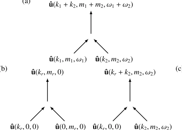
Figure 2.1: Representation of nonlinear interactions between triadically consistent velocity modes, (a) for the canonical case, where k1,k2,m1,m2, ω1, ω2 , 0, (b)
for the case of periodic roughness, where direct interactions give rise to a station-ary response, for example the interactions of the velocity response at roughness wavenumbers (kr,0,0) and (0,mr,0) giving rise to a response at (kr,mr,0), and (c)
again for periodic roughness, for the case of a static mode and a spatio-temporally varying one giving rise to a response at a spatio-temporally varyingK.
Triadic Interactions
The expression ˆu(y;K) can be interpreted as the wall-normal (complex) variation of wave-like spatio-temporally varying velocity modes with streamwise, spanwise and temporal wavenumbers given byK. The last term in Equation 2.17 accounts for nonlinear interactions coupling between such modes to give a response atK. These interactions can be effectively described in terms of triads; for a pair of modes with wavevectors K1 and K2 to interact with a mode with wavevector K, they must be triadically-consistent, i.e. K1+ K2 = K. This triadic relation is illustrated for the canonical case in Figure 2.1(a), wherek1,k2,m1,m2, ω1, ω2 , 0, i.e. all deviations
from the mean have non-zero spatial and temporal variations. The full nonlinear term at Kcorresponds to the integral over all triadically consistent pairs.
am-w+(x,h(x,z),z)= w0(x,0,z)+a(cos(krx) cos(mrz)∂yw0(x,0,z)+w1(x,0,z))+· · ·= 0,
(2.53)
w0,
w0(x,0,z)=0, (2.54)
andw1,
w1(x,0,z)=−cos(krx) cos(mrz)∂yw0(x,0,z). (2.55)
The expansion of the wall-normal velocity,
v+(x,h(x,z),z)= v0(x,0,z)+a(cos(krx) cos(mrz)∂yv0(x,0,z)+v1(x,0,z))+· · · =0,
(2.56)
gives a boundary condition for orderO(1) ,
v0(x,0,z)=0, (2.57)
as well as orderO(a),
v1(x,0,z)=−cos(krx) cos(mrz)∂yv0(x,0,z). (2.58)
Applying Equations 2.50, 2.53, and 2.56 to the continuity equation for incompress-ible flow yields the following expression at orderO(1):
0= ∂xu0(x,0,z)+∂yv0(x,0,z)+∂zw0(x,0,z). (2.59)
Substituting Equation 2.58 and solving forv1 gives
v1(x,0,z)= cos(krx) cos(mrz) (∂xu0(x,0,z)−∂zw0(x,0,z)). (2.60)
0=∂x
acos(krx) cos(mrz)∂yu0(x,0,z)+u1(x,0,z)
+acos(krx) cos(mrz)∂2yv0(x,0,z)+a∂yv1(x,0,z)
+∂z
acos(krx) cos(mrz)∂yw0(x,0,z)+aw1(x,0,z)
.
(2.61)
Taking the terms with subscript zero to be the spatio-temporally averaged veloc-ity hu+i which is constant in x and z and which obeys symmetry in z, boundary conditions for the velocity components at orderO(a) reduce to
u1(x,0,z)= −cos(krx) cos(mrz)∂yhu+i, (2.62)
w1(x,0,z)=0, (2.63)
v1(x,0,z)=0, (2.64)
and
∂yv1(x,0,z)=−acos(krx) cos(mrz)∂2yhv
+i=0. (2.65)
Applying the definition for vorticityηyields
η1(x,0,z)= mrcos(krx) sin(mrz)∂yhu+i. (2.66)
After performing spatial Fourier transforms in thexandzdirections, the orderO(a) boundary conditions give the boundary conditions for the (k,m, ω) = (±kr,±mr,0)
resolvent modes, which have zero frequency and are coherent with the roughness. Higher-order terms in the expansion will give boundary conditions for (k,m, ω) =
(±2kr,±2mr,0),(±2kr,0,0), etc. The boundary conditions differ from the
Volume penalization within the resolvent method
Another method of incorporating the rough wall boundary condition into the re-solvent was introduced by Luhar and Chavarin [12], using a volume penalization approach that is similar to the immersed boundary method for fluid simulations. The technique sets the zero point of the wall-normal coordinateyat the very lowest point of the roughness. A scalar permeability K is assigned to each point in the volumey> 0, which is<<1 within the solid surface of the wall and infinite above the wall. An additional Darcy-type linear body force is added to the momentum equation,
∂u+
∂t+ +u
+· ∇u+= −∇p++ 1 Reτ
∇2u+−K−1u+, (2.67)
which is linearly proportional to local velocity and the inverse of permeability. While the technique is applicable to general roughness, Luhar and Chavarin con-sider only streamwise-constant roughness, and this section will reproduce their derivation without extending it to three-dimensional roughness. The inverse per-meability K−1 will then be a function of y and z, and representable as a sum of
Fourier modes inz:
K−1(y,z)=
∞
X
n=−∞
an(y) exp(inmrz). (2.68)
The time-average streamwise velocity can be represented in the same way,
u+(y,z)=
∞
X
n=−∞
un(y) exp(inmrz), (2.69)
with the other components of mean velocity taken to be zero. Luhar and Chavarin calculate the mean velocity field using an eddy viscosity.
computationally expensive, as the resolvent matrix for a domain withN discretiza-tion points in they-direction andNpoints in another spatial direction will be of size
N2×N2, compared toN×N for the conventional resolvent. This work will employ only the conventional, one-dimensional resolvent operator.
2.3 Experimental Methods
Run Conditions
Experimental rough- and smooth-wall boundary layer experiments were performed in the Merrill wind tunnel at Caltech. The test section of the wind tunnel measures 2440mm in the streamwise direction, with a square cross-section that measures 610mm on each edge. The boundary layers were developed over an acrylic plate which spans the width of the wind tunnel. The boundary layers are tripped 19mm
downstream of the parabolic leading edge by a 0.76mmdiameter piano wire glued to the plate surface, as described by Duvvuri [17]. Hot-wire measurements were taken 1250mmdownstream of the trip. The pressure gradient is controlled by a de-formable ceiling, which is adjustable at ten points along the test section. Freestream velocityU∞ and velocity profiles were measured with hot-wire anemometry.
Mo-mentum thicknessθand 99% thicknessδwere calculated directly from the velocity profiles (or spatially-averaged velocity profiles in the case of the rough-wall mea-surements). The friction velocityuτwas determined in the smooth case by empirical relations to the momentum thickness. In the rough cases, uτ was determined by a single iteration of the modified Clauser method [56] as described algorithmically by LeHew [37]. Physically, there is likely spatial variation in the shear stress at the wall, but the result of this calculation is an estimate of spatially-averaged shear stress at the wall, consistent with its definition in the roughness literature. Smooth-and rough-wall run conditions are summarized in Table 2.1. Run conditions were selected to roughly match the friction Reynolds numberReτ in order to fulfill the conditions for wall similarity given by Raupach et al. [60]. The acceleration param-eterK = 4Uν3∞ρ
d p
dx, as defined by DeGraaf and Eaton [15], was of the order 1×10
−8
Table 2.1: Run Conditions
Set U∞ δ ν θ uτ Reδ Reτ Reθ
(m/s) (mm) (m2/s) (mm) (m/s)
Smooth 18.0 24.4 1.53E-05 3.03 0.71 29000 1100 3600 R1M 20.3 23.4 1.56E-05 2.82 0.84 30000 1300 3700 R2M 16.3 24.8 1.56E-05 3.08 0.74 26000 1200 3200
Geometry
Two roughness surfaces were 3D-printed for wind-tunnel testing. The first sur-face, labeled R1M in Tables 2.1-2.3, was printed with a spatially-varying height
hR1M(x,z) consisting of a single Fourier mode of amplitude a which varies in x
and zwith a single wavelength λx and λz in each direction, respectively, as given
in Equation 2.75. A second roughness surface, labeled R2M, was designed with heighthR2M(x,z) consisting of a single streamwise-varying Fourier mode with
am-plitudeaand wavelengthλx added to a single spanwise-varying Fourier mode with
identical amplitudea and wavelengthλz, as given in Equation 2.76. In each case,
they= 0 plane is located at the mean roughness height.
hR1M(x,z)=acos(2πx/λx)·cos(2πz/λz). (2.75)
hR2M(x,z)= acos(2πx/λx)+acos(2πz/λz). (2.76)
(a) An illustration of the R1M roughness geometry, with exaggerated y-dimension.
(b) Hot-wire measurement locations within a single streamwise and span-wise wavelength of the roughness. Lighter colors denote
higher-than-average roughness elevation, with peaks aty=182µm, while darker colors
denote lower-than-average roughness elevation, with troughs at y=-182
µm. Green circles show the locations of hot-wire traverses in y, while red circles show locations for which the velocity statistics can be imputed from the hot-wire data using symmetries of the roughness geometry.
Table 2.2: Roughness Geometry Parameters
Set λx λz a λ+x λz+ a+ λx/δ λz/δ a/δ δ/a
(mm) (mm) (mm)
R1M 20 10 0.182 1080 540 10 0.86 0.43 0.008 128 R2M 20 10 0.182 950 475 9 0.81 0.40 0.008 136
(a) An illustration of the R2M roughness geometry, with exaggerated y-dimension.
(b) Hot-wire measurement locations within a single streamwise and span-wise wavelength of the roughness. Lighter colors denote
higher-than-average roughness elevation, with peaks aty=364µm, while darker colors
denote lower-than-average roughness elevation, with troughs at y=-364
µm. Green circles show the locations of hot-wire traverses in y.
Figure 2.4: R1M traverse hot-wire probe setup. The pressure probe “A” is used for hot-wire calibration in the freestream. The hot-wire probe holder “B” holds a hot-wire probe (not shown). Linear stages “C” and “D” allow for streamwise and spanwise adjustment of the hot-wire probe. The post “E” extends below the roughness surface and is mounted to a powered traverse that allows wall-normal adjustment during the experiment.
Figure 2.5: R2M traverse hot-wire probe setup. The pressure probe “A” is used for hot-wire calibration in the freestream. The hot-wire probe holder “B” holds a hot-wire probe (not shown). The collar “C” holds the probe holder in place with a set screw, allowing streamwise adjustment. It is mounted on rod “D” with another set screw, allowing for spanwise adjustment of the hot-wire probe. The post “E” extends below the roughness surface and is mounted to a powered traverse that allows wall-normal adjustment during the experiment.
Hot-wire Parameters
fixed below the test surface and extended through a port cut into the roughness and test section. A traverse allowed measurements at multiple wall-normal distances during a single test run, and the hot wire probe was adjusted between experiments in the streamwise and spanwise directions to alter the position of the measurement volume. For each station and y-location, 100s of streamwise velocity data were recorded using a 55P05 boundary-layer type hot-wire probe and Dantec Streamline Pro anemometer, equal to 74,000 eddy turnover times (δ/U∞). Hot-wire
measure-ment parameters including sampling rate fs, active length L, active diameter D, and
hot-wire low-pass filter cutofffrequency fc are detailed in Table 2.3 below along
with their associated non-dimensional values.
Single-Mode Roughness
For the R1M case, two micrometer-equipped linear stages labeled “C” and “D” were used to adjust the streamwise and spanwise position of the hot-wire probe holder “B” between runs, as shown in Figure 2.4. Twelve wall-normal traverses were performed within a single period of roughness, denoted by green circles in Figure 2.2b. The velocity statistics for twenty additional locations, shown in red circles, can be imputed from the hot-wire data using symmetries of the rough-ness geometry and the assumption of a non-developing periodic flow. For exam-ple, under these assumptions, the red circle located at (x,z) = (0mm,5mm) is ex-pected to have velocity statistics which are identical to those at the measured lo-cation (x,z) = (10mm,5mm), exploiting the symmetry in this geometry of a 10mm
streamwise translation combined with a reflection in z. This set of 32 points al-lows for spatial phase averaging to decompose the field into components directly correlated with the wavenumber content of the roughness. Specifically, performing a Fourier transform of mean velocity ¯u(x,y,z) in x and a cosine transform in z(to ensure spanwise symmetry) yields a set of spatial Fourier modes ˆ¯u(y,k,m), where k is the streamwise wavenumber and m the spanwise wavenumber. Following the Nyquist criterion, one can determine from the eight-by-four grid of data modes with
k= 0,kr,2krandm= 0,mz,2mr, wherekr andmrare the streamwise and spanwise
roughness wavenumbers, respectively. A series of time-averaged velocity profile measurements were taken at 10mmincrements across the span of the tunnel to ver-ify streamwise homogeneity in run conditions around the measurement volume.
above the local roughness height. Spatial averages and spatial Fourier transforms are performed in this paper only for values of y for which data from all measurement stations exist. As a result, the lower bound onyfor these quantities is 150µmabove the crest of the roughness, y= 334µm= 0.01δ. Estimated error fory-positioning of the hot-wire probe is±9µm. The estimated errors for the (x,z) positioning of the hot-wire are 0.3mmin each dimension.
Two-Mode Roughness
For the R2M case, the hotwire probe was adjusted between runs in the streamwise direction by sliding the hot-wire probe holder “B” within its collar “C”, while ad-justment in the spanwise directions was accomplished by moving the collar along a spanwise rod “D”, as shown in Figure 2.5. Eight wall-normal traverses were per-formed over a single period of roughness, in a grid that spanned four stations in the streamwise direction and two stations in the spanwise direction, as shown in Figure 2.3b. This set of points allows for spatial phase averaging to decompose the field into components directly correlated with the wavenumber content of the roughness. Specifically, performing a Fourier transform of mean velocity ¯u(x,y,z) in x and a cosine transform in z (to ensure spanwise symmetry) yields a set of spa-tial Fourier modes ˆ¯u(y,k,m), where k is the streamwise wavenumber and m the spanwise wavenumber. Following the Nyquist criterion, one can determine from the four-by-two grid of data modes withk=0,kx andm=0,kz, wherekxandkzare
the streamwise and spanwise roughness wavenumbers, respectively.
The origin of the y-axis is taken to be the spatial average of the roughness height, i.e. h=0 in Equation 2.76. Hot-wire measurements were taken starting at 150µm
above the local roughness height. Spatial averages and spatial Fourier transforms are performed in this paper only for values of y for which data from all measurement stations exist. As a result, the lower bound onyfor these quantities is 150µmabove the crest of the roughness,y=514µm=0.02δ. Estimated error for y-positioning of
Table 2.3: Hot-wire acquisition parameters
Set fs fs+ L D L/D L+ fc fc+
(kHz) (mm) (µm) (kHz) Smooth 60 1.8 1.25 5 250 56 30 0.9
R1M 60 1.3 1.25 5 250 67 30 0.9
C h a p t e r 3
EXPERIMENTAL MEASUREMENT OF PERIODIC ROUGH
WALL TURBULENT BOUNDARY LAYERS
This chapter will present the measured flow characteristics of the simply periodic rough wall boundary layer. Spatially-averaged profiles of time-averaged velocity and velocity statistics reveal the bulk effect of roughness on the boundary layer. The spatially-varying parts of these fields are correlated to the periodic roughness, revealing the direct effect of the roughness on boundary layer physics. In a novel contribution to the field, the spatial variation of the streamwise power spectrum is also correlated to the roughness, showing the modulation of individual scales in the flow by the roughness.
3.1 Spatio-temporal average flow statistics
The velocity, velocity deficit, and variance profiles for the spatio-temporal averages, i.e. hu¯+i(y), U∞+ − hu¯+i(y), andhu0u0
+
i(y), are shown for the smooth and the rough wall cases in Figures 3.1 and 3.2. For the smooth wall which is homogeneous in x
andz, hQ¯i(y)= Q¯(y) for all quantities Q. There are significant differences between the spatio-temporal average profiles over the rough and the smooth wall case for both velocity deficit and variance. As would be expected, there is a significant de-viation between the profiles close to the wall, but there is also a marked divergence between the two cases well outside the traditional roughness sublayer. For the R1M case, the lack of collapse extends to approximatelyy/δ=0.4 for the velocity deficit
andy/δ = 0.05 for the variance. The lack of collapse extends through most of the
boundary layer until approximatelyy/δ= 0.6 for the R2M case.
Contrary to the majority of results associated with three-dimensional, multi-scale roughnesses, the influence of the wall is felt far beyond the usual estimate of a roughness sublayer, 5 times the roughness height k [32], which is equal to ap-proximately y/δ = 0.08 for both rough cases. This appears inconsistent with the
het-(a)
(b)
Figure 3.2: Spatio-temporally averaged velocity variance of rough and smooth walls
erogeneous roughnesses with coherence in the streamwise and spanwise directions, this roughness has large length-scales corresponding to the roughness wavelengths. These large length scales are not separated in scale from the boundary layer thick-ness, so the Townsend hypothesis does not hold. Consistent with Volino et al. [72], the R2M roughness with a spanwise-aligned mode creates the most persistent devi-ation from Townsend’s hypothesis.
3.2 Spatial variation of the time-averaged velocity field
The spatially-averaged quantities shown in Figures 3.1 and Figure 3.2 obscure the secondary flow associated with the roughness, which takes the form of substantial spatial variation in the mean velocity outside the roughness sublayer. By performing a number of traverses at stations separated in x and z within a single period of roughness, at the locations shown in Figures 2.2b and 2.3b, it is possible to map (by spatial interpolation) the streamwise and spanwise variation in the time-averaged velocity, ˜¯u+(x,y,z).
both rough geometries, as defined in Figures 2.2b and 2.3b. Color scales are not kept consistent between the two plots because no similarity is expected between two different roughnesses for raw mean velocity (as opposed to the velocity deficit form shown in Figure 3.1b). For the R1M case, this streamwise-aligned plane is one with maximum variation in the roughness height, hitting both absolute maxima and minima. For the R2M case, this is a streamwise-aligned plane that sits over a crest in the spanwise roughness (Figure 2.3). In both geometries, the position
x/λx = 0 corresponds to a peak in the streamwise direction while x/λx = 0.5
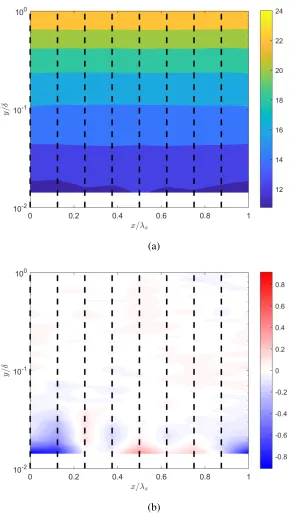
corresponds to a trough in the streamwise direction. There is clear variation in mean velocity close to the wall, which is made clear by plotting the same data with the spatial average subtracted, ˜¯u+(x,y,z), in Figures 3.3b and 3.4b. The pattern in each case is very close to singly-periodic with a wavelength matching the roughness wavelength. Note that thex-averages of the data plotted in Figures 3.3b and 3.4b are not necessarily identically zero, as there are other planes of data which contribute to the spatial average.
In the R1M case, the streamwise and spanwise variation in the time-averaged ve-locity, ˜¯u+(x,y,z), is faster over a trough in the roughness located at x/λx = 0.5 and
slower over a peak in roughness located at x/λx = 0. This is consistent with a
“profile displacement” model of velocity variation, in which an elevated roughness element displaces a velocity profile upwards, causing lower mean velocities at a giveny.
For the R2M case, close to the wall, there is a strong velocity deficit (negative ˜¯
u+(x,y,z)) located on the rising portion of the peak. Further from the wall, velocity deficits sit over troughs while pockets of excess velocity sit over peaks. The place-ment of positive ˜¯u+(x,y,z) over a roughness peak is consistent with a “streamtube deformation” model of velocity variation, in which an elevated roughness element accelerates the flow above it by locally compressing streamtubes. This effect may be more pronounced in the R2M case compared to the R1M case due to its streamwise-constant mode: the streamtubes cannot curve around the spanwise-streamwise-constant peaks.
3.3 Signature of the roughness geometry in the spatial variation of the
time-averaged velocity field
(a)
(b)
Figure 3.3: Spatial representations for the R1M case of (a) the mean velocity field ¯
u+(x,y,z) on the z = 0 plane, (b)the spatial variation in the mean velocity field ˜¯
u+(x,y,z) on the z = 0 plane. Red contours indicate a region in which the flow is faster than at other points at the same y-location. Measurement locations at
(a)
(b)
Figure 3.4: Spatial representations for the R2M case of (a) the mean velocity field ¯
u+(x,y,z) on the z = 0 plane, (b)the spatial variation in the mean velocity field ˜¯
u+(x,y,z) on the z = 0 plane. Red contours indicate a region in which the flow is faster than at other points at the same y-location. Measurement locations at
¯
u+(x,y,z) in xand a cosine transform inz(to ensure spanwise symmetry) yields a set of stationary velocity Fourier modes ˆu+(y,k,m,0), where k is the streamwise wavenumber and m the spanwise wavenumber, and with zero frequency. Follow-ing the Nyquist criterion, one can determine from the eight-by-four grid of data for the R1M case modes with k = 0,kr,2kr andm = 0,mz,2mr, where kr and mr are
the streamwise and spanwise roughness wavenumbers, respectively. The R2M case permits calculation of modes withk = 0,kr andm = 0,mr. There is no indication
of such static velocity modes in smooth-wall data for the same wind tunnel.
Contributions to the R1M spatial variation in mean velocity ˜¯u+(x,y,z) from resolv-able spatial modes are plotted as spatial reconstructions in Figures 3.5a - 3.5d. Modes for which (k,m) = (kr,0),(0,mr) contribute identically zero to observed
˜¯
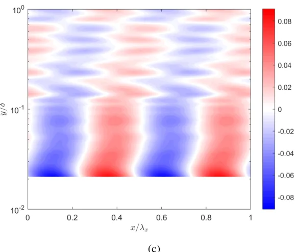
u+(x,y,z) due to symmetry. Stationary velocity mode ˆu+(y;kr,mr,0) is the
station-ary velocity mode with the highest amplitude, reaching 0.54 in inner units at the lower limit of the measurement volume and accounting for most of the spatial vari-ation in mean velocity. This is expected, as this is the only mode with the same frequency content as the roughness, allowing the roughness geometry and this ve-locity mode to be connected through linear mechanisms. The qualitative features of the full ˜¯u(x,y,z) field are evident in this mode, including the x- andy- locations of the velocity deficits and the change in phase withy. This mode also decays more quickly withythan the other wavenumbers.
Stationary velocity modes ˆu+(y; 2kr,2mr,0), ˆu+(y; 2kr,0,0),and ˆu+(y; 0,2mr,0) for
case R1M are plotted in Figures 3.5b-3.5d. They are substantially weaker than ˆ
u+(y;kr,mr,0), as they can only be formed by non-linear interactions within the
flow. Compared to ˆu+(y;kr,mr,0), they also decay more slowly inyand have less
phase variation. The spanwise-varying-only stationary velocity mode ˆu+(y; 0,2mr,0)
is constrained by symmetry from varying continuously in phase, but does notably invert in sign aroundy/δ =0.05.
The relative uncertainty in the amplitude of the R1M mode ˆu+(y;kr,mr,0) is 6% of
(a)
(b)
Contributions to the R2M spatial variation in mean velocity ˜¯u(x,y,z) from resolv-able spatial modes are plotted as spatial reconstructions in Figures 3.6a - 3.6c. For the R2M case, the streamwise-varying-only mode, ˆu+(y;kr,0,0), has the largest
(c)
(d)
Figure 3.5: Spatial representations for the R1M case of (a) the stationary ve-locity Fourier mode ˆu+(y;kr,mr,0), (b) the stationary velocity Fourier mode
ˆ
u+(y,2kr,2mr,0), (c) the stationary velocity Fourier mode ˆu+(y,2kr,0,0), and (d)
the stationary velocity Fourier mode ˆu+(y,0,2mr,0). Red contours indicate a region
amplitude peaking near the wall and the high-speed regions over roughness peaks. The mode ˆu+(y;kr,0,0) attains a maximum amplitude of 0.23 inner units at the
lower limit of the measurement volume and decays slowly in amplitude withy. The other stationary velocity mode ˆu+(y; 0,mr,0) with a linear connection to the
rough-ness geometry, shown in Figure 3.6b, also has a fairly large amplitude, peaking at 0.11 aty/δ=0.26. Spanwise symmetry constrains the phase of this mode such that
a maximum in velocity must lie directly over either a roughness crest or a roughness trough. In this case, regions of high velocity in this mode lie above the roughness crests in thez-direction and permeate the entire boundary layer. This is consistent with observations of high-momentum zones in streamwise-aligned roughnesses by Vandervel and Ganapathisubramani [71] and others. The mode ˆu+(y;kr,mr,0) is the
smallest measured stationary velocity mode, as it can be created only by non-linear interactions involving the other stationary modes. It attains a maximum amplitude of 0.09 at the lower limit of the measurement volume and changes only slightly in phase withy.
The relative uncertainty in the amplitude of the R2M mode ˆu+(y;kr,0,0) has a
max-imum of 28% of the local amplitude at the lower limit of the measurement volume, and the relative uncertainty is below 10% for all y/δ >0.073. The uncertainty is mostly due to errors in the y-positioning of the hot-wire probe. The other measur-able spatial Fourier modes ˆu+(y; 0,mr,0) and ˆu+(y,kr,mr) have relative uncertainties
of 91% and 83%, respectively, at the lower limit of the measurement volume. The relative uncertainty of ˆu+(y; 0,mr,0) is below 25% for ally/δ >0.048, while
uncer-tainty in ˆu+(y,kr,mr) persists throughout the boundary layer.
3.4 Spatially-averaged velocity power spectra
Due to the highly time-resolved instantaneous velocity data available at each mea-surement point, the spatial distribution of streamwise stressu0u0(x,y,z) can be
de-composed into contributions from each individual frequency measured in the flow. We consider first the spatial average over the roughness unit of the power spectrum Φ(y,x,z, ω) of the streamwise fluctuating velocity,u0(x,y,z,t).
fil-(a)
(c)
Figure 3.6: Spatial representations for the R2M case of (a) the mean velocity spatial Fourier mode ˆu+(y;kx,0,0), (b) the mean velocity spatial Fourier mode
ˆ
u+(y,0,kz,0), and (c) the mean velocity spatial Fourier mode ˆu+(y,kx,kz,0). Red
contours indicate a region in which the flow is faster than at other points at the same y-location.
ter was applied to the power spectra with a width equal to one tenth of a decade in wavenumber in order to smooth the data and simplify the comparison between cases. Consistent with the results for velocity variance, the R1M case is very simi-lar to the smooth-wall case while the R2M boundary layer contains less energy than the smooth case at all values of (y, ω). Consistent with the observations of Chan et
al. for sinusoidal roughness in pipe flow [11], the R2M roughness, with substantial secondary flow throughout the boundary layer, has a power spectrum that is shifted toward higher frequencies.
3.5 Signature of the roughness geometry in the velocity power spectra
Just as with mean velocities earlier in the chapter, the same spatial variation, i.e. the spatial dependence that is correlated to the roughness geometry and thus stationary in space, can be examined for the power spectrum of the stress by decomposition into spatial Fourier modes. We examine the contributions to this spatial dependence by wavenumber of the time-dependent signal by examining the spectral content of the variation, i.e.dωΦ
+
ap-(a)
(c)
Figure 3.7: Comparison of spatially-averaged premultiplied angular frequency power spectra hωΦ(y, ω)ifor (a) the smooth-wall case, (b) the R1M case and (c) the R2M case .
plying Welch’s method to experimental data. As with the spatially-averaged spec-tra, these plots were smoothed with a moving average filter with a width equal to one tenth of a decade in frequency. A larger filter width would result in additional smoothing, at the cost of reducing frequency precision. It must be stressed that the stationary velocity Fourier modes shown earlier do not contribute to the power spectra. The only velocity Fourier modes which contribute to the measured power spectrum are modes with non-zero frequency which convect past the hotwire. The finite frequency associated with these modes ensures that they have no linear in-teraction with the zero-frequency static roughness. With reference to the triadic interactions shown in Figure 2.1(a), note that contributions to the spatio-temporal average stress can only arise from interactions with (k2,m2, ω2) = −(k1,m1, ω1).
A temporally stationary but spatially varying stress at (k1 +k2,m1+m2,0) can be obtained from pairs of velocity Fourier modes with wavenumbers K1,K2such that (k1,m1, ω1)= (k2,m2,−ω1); this is the subject of this section.
The quantity |ωbΦ+(y, ω;k,m)|is identically zero for a smooth wall with non-zero
(a)
(b)
in ω). It is a measurement of the extent to which the kinetic energy present at a particular scale in the flow is modulated in space by interaction with the roughness-correlated stationary modes, so we will name it the “scale modulation” of the flow at a particular set of wavenumbers.
(c)
(d)
Figure 3.8: Magnitude of the R1M scale modulation|ωbΦ+(y, ω;k,m)|for (k,m) =
spatial variation in power spectra is most pronounced for (k,m)= (kr,mr), as shown
in Figure 3.8a. Notably, the scale modulation at this wavenumber is concentrated in a relatively small region in (ω,y) space, aroundω+ = 0.02 and lying against the lower boundary of the measurement volume. That the scale modulation is much more concentrated than the average power spectrum from Figure 3.7b implies that certain scales are preferentially modulated by the stationary velocity Fourier modes. The modulation is also focused at low y, like the corresponding velocity Fourier mode. The scale modulation for (k,m) = (0,2mr), from Figure 3.8d is similarly
concentrated, but at a higher wavenumber aroundω+ = 0.1. The scale modulation also reaches into fairly large y-values, like the velocity Fourier mode for (k,m) = (0,2mr). The other wavenumbers show very little scale modulation at all. This
implies that the strength of the scale modulation, as well as the region of preferential modulation, are strong functions of roughness wavenumber.
For the R2M case, the streamwise-varying-only mode with (k,m)= (kr,0) displays
the strongest scale modulation, as shown in Figure 3.9a. There are two lobes of high scale modulation, centered at ω = 0.01,0.08. The scale modulation for (k,m) = (0,mr), from Figure 3.9b, also shows two lobes, but separated inyas well. Here, the
scale modulation extends almost to the boundary layer edge, like the corresponding velocity Fourier mode (k,m)= (0,mr) in Figure 3.6b. The remaining wavenumber
(k,m)=(kr,mr) shows little scale modulation.
3.6 Discussion
pro-(a)
(c)
Figure 3.9: Magnitude of the R2M scale modulation|ωbΦ+(y, ω;k,m)|for (k,m) =
(a)(kr,0) (b)(0,mr) (c)(kr,mr).
duce the scale modulation recorded in this chapter. The general correspondence between the wall-normal extent of the stationary velocity Fourier modes and that of the scale modulation suggests that these stationary velocity modes are responsible, through the triadic interactions described in Chapter 2.
C h a p t e r 4
MODELING AND SCALING OF STATIC VELOCITY FOURIER
MODES
The chapter evaluates the suitability of most-amplified resolvent modes for the pur-pose of modeling the spatial variation in mean velocity induced by a periodic rough-ness. With a link established between the static resolvent modes and the observed spatial Fourier modes of mean velocity, the scaling of these modes with respect to roughness wavenumber and Reynolds number is explored. While the scaling of traveling-wave resolvent modes with Reynolds number has been characterized by Moarref et al. [46], modeling efforts here require static resolvent modes withω= 0, whose scaling have not been studied.
4.1 Resolvent Modes as Models for Velocity Fourier Modes in Wall-Bounded
Turbulence
Most-amplified resolvent modes, as measured by the associated singular value, have been successfully used to model convecting velocity Fourier modes associated with particular wavenumber-frequency vectors. Applications have included opposition control [39], energy density scaling [46], and response to time-periodic perturba-tions [17]. In this chapter, resolvent modes will be used to model non-linear (tri-adic) interactions within periodic rough-wall turbulent boundary layers. This will require, at minimum, a single stationary resolvent mode with non-zero wavenumber and zero frequency to model the stationary velocity mode induced by the roughness, as well as two convecting resolvent modes with non-zero frequency which are tri-adically compatible with the stationary mode.
This weighting vectorγcan then be used to create a best-fit mode by left-multiplying the basisψ.
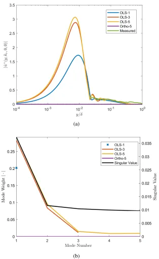
The least squares regression is performed using MATLAB’s built in “mldivide” function. As the result depends on the selection of basis vectors, regressions are performed using the most amplified resolvent response mode, the 3 most-amplified modes, and the 5 most-amplified modes with non-zerou-components to check for robustness. Modes with zero-valuedu-velocity fields are discarded. For the R1M case with (k,m)=(kr,0) and the R2M case with (k,m)=(kr,0), the modes with the
second, third, fifth, seventh, and ninth highest singular values were discarded for that reason. All other cases considered here had no discarded modes. Both the basis vectors and the observed ˆu+ field are sampled at 800 evenly-spaced points throughout the measurement volume before performing the regression.
In both methods, the basis of resolvent response modes φ is calculated from the resolvent as described in Section 2.2 with N = 800, with zero frequency and an appropriate wavenumber. The velocity profile used as a input to the resolvent is taken to be the observed spatio-temporally averaged velocity field for the appropri-ate roughness geometry, with linear interpolation to zero velocity at zero y below the measurement volume.
The results of both fitting processes for all the observable wavenumbers are plotted in Figures 4.1-4.7. Although all plots show only absolute values, phase information for the observed modes and for the basis was used for all fits.
Figure 4.1a shows the amplitude of the observed stationary velocity Fourier mode ˆ
u+(y;kr,mr,0) for the R1M roughness. This mode presents clear challenges for
(a)
(b)
Figure 4.1: R1M roughness, (k,m) = (kr,mr) a) Amplitude of measured