MASTER THESIS
OSCILLATORY FLOW
IN JET PUMPS:
SETUP DESIGN
AND EXPERIMENTS
Mahening Citra Vidya
FACULTY OF ENGINEERING TECHNOLOGY LABORATORY OF THERMAL ENGINEERING EXAMINATION COMMITTEE
Prof.dr.ir. T.H. van der Meer (chairman) Ir. J.P. Oosterhuis (internal member) Dipl. Ing. S. Bühler (internal member) prof.dr.ir. A. Hirschberg (external member)
i
MASTER THESIS
OSCILLATORY
FLOW
IN
JET
PUMPS:
SETUP
DESIGN
AND
EXPERIMENTS
AUTHOR Mahening Citra Vidya
EXAMINATIONCOMMITTEE
Prof. dr. ir. T.H. van der Meer (chairman) Ir. J.P. Oosterhuis (internal member) Dipl. Ing. S. Bühler (internal member) Prof. dr. ir. A. Hirschberg (external member)
UNIVERSITYOFTWENTE
Faculty of Engineering Technology Department of Mechanical Engineering Drienerlolaan 5
7522 NB Enschede
iii
PREFACE
Firstly, I would like to express my gratitude to my daily supervisor, Joris Oosterhuis, to whom I am so much indebted. This thesis would not be possible without his guidance. His positive support, discussion and corrections are greatly appreciated. I would like to thank Theo van der Meer, who allowed me to work on this project and always encouraged me to discuss during our weekly meeting. His guidance since the first time I arrived in this university until my graduation day will not be forgotten. I am also grateful to Simon Bühler, for carefully reading the thesis draft and providing important comments as well as discussions.
This thesis consists of design process and experimental work in the Thermal Engineering Laboratory. During these nine months, I gain a lot of knowledge and insight in the field of thermoacoustic. The design process required me to learn Matlab and deal with the scripts, which provide me with valuable skill. I also have more experience in working with the experimental setup, for which I am very grateful for the opportunity. Generous support from the Indonesian Ministry of Education Scholarship that made me possible to reach this opportunity is gratefully acknowledged.
The experimental works would not be possible to perform without the help of Henk‐Jan Moed and Robert, who assisted me with the experimental setup, constructed the flow visualization test section and helped me during my time in the laboratory. Special thanks to my partners in the lab, Frederieke and Koen, who helped me to obtain the experimental data. Furthermore, I would like to thank the guys in N248: Rob, Sjoerd, Niek and Gerrald, who were there during the whole thesis period and of course, thank you for teaching me klaverjas and for giving me a very good time in our room. I also thank Riza who supplied me with enormous amount of food, my colleagues in Thermal Engineering, my housemates and all Indonesian people in Enschede.
Finally, I acknowledge my thanks to my parents and my wonderful brother for their endless love and support.
v
3.2.2. Acoustic power dissipation measurement ... 46
3.2.3. Estimation of experimental and ... 47
3.3. Results ... 48
3.3.1. Pressure and power measurement ... 49
3.3.1.1. Effect of taper angle ... 49
3.3.1.2. Effect of number of holes ... 53
3.3.1.3. Effect of wave phasing ... 58
3.3.1.4. Estimation of experimental minor loss coefficients ... 59
3.3.2. Flow visualization ... 62
3.3.2.1. Description of flow patterns ... 62
3.3.2.2. Vortex detection and propagation speed calculation ... 65
3.4. Summary... 68
CHAPTER 4 CONCLUSION AND RECOMMENDATION... 70
4.1. Conclusion ... 70
4.2. Recommendation ... 71
BIBLIOGRAPHY ... 73
APPENDIX A TRAVELING WAVE TERMINATION MODEL ... 76
APPENDIX B EXPERIMENTAL RESULTS OF PRESSURE AND POWER MEASUREMENT ... 83
APPENDIX C CALCULATION OF INNER WALL SURFACE AREA ... 92
vii
Figure 3.13 Schematic diagram of two parallel jet streams [32]. ... 56
Figure 3.14 Power dissipation plotted against pressure drop. ... 57
Figure 3.15 Effect of wave phasing on pressure drop for low taper angle jet pump. ... 58
Figure 3.16 Effect of wave phasing on pressure drop for high taper angle jet pump. ... 58
Figure 3.17 Effect of wave phasing on power dissipation for the 18° jet pump. ... 59
Figure 3.18 Total minor loss coefficient of the jet pump samples. ... 60
Figure 3.19 Experimental and of jet pump samples. ... 61
Figure 3.20 Experimental results of Petculescu and Wilen [7]. ... 61
Figure 3.21 Gas oscillation. ... 63
Figure 3.22 Trail of smoke sucked into the jet pump. ... 64
Figure 3.23 Outburst flow. ... 65
Figure 3.24 Schematic of vortex ring propagation and rotational direction. ... 66
Figure 3.25 Vortex edge detection. ... 67
Figure 3.26 Vortex propagation speed as a function of frequency. ... 68
Figure 0.1 A traveling wave termination connected to the main tube in series [11]. ... 76
Figure 0.2 Comparison of model implementation and van der Eerden’s result [11]: ... 77
Figure 0.3 Pressure amplitude at the traveling wave termination. ... 78
Figure 0.4 Influence of end correction. ... 79
Figure 0.5 Relation between tube radius, length, absorption coefficient and working frequency. ... 80
Figure 0.6 The comparison of foam effect at 100 Pa and 600 Pa. ... 81
Figure 0.7 Schematic of the backward traveling wave. ... 81
viii
LIST
OF
TABLES
Table 2.1 Design limitations. ... 27
Table 2.2 List of working frequency and absorption coefficient for varied radii. ... 28
Table 2.3 List of working frequency and absorption coefficient for varied tube length. ... 29
Table 2.4 Final design of the traveling wave termination. ... 29
Table 2.5 List of working frequencies at specified temperature. ... 31
Table 2.6 Smoke fluid selection table. ... 38
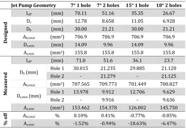
Table 3.1 Designed and measured jet pump geometry. ... 43
Table 3.2 xJP values for each jet pump sample. ... 44
Table 3.3 Effectiveness constants for determining the velocity amplitude (m/(Pa.s)). ... 45
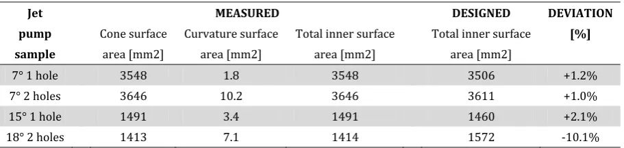
Table 3.4 Comparison of actual and designed inner wall surface area. ... 55
11
INDICES Cold
Hot Minor loss Mean Expansion Contraction Narrow‐end Wide‐end
Flow in‐to the narrow‐end Flow out‐of the narrow‐end curvature
Jet pump Maximum Minimum
Backward propagating wave Forward propagating wave Geometrical
Effective Total Average Vena contracta
ABBREVIATION TAP Thermo Acoustic Power
13
sectional device which is known as a jet pump is studied. Various jet pump samples are tested in the experimental setup for this thesis.
The experimental setup used to perform experiments in the scope of this thesis was originally established at the Technical University of Eindhoven. This setup is now being used at the University of Twente. The experimental setup consists of three main parts: the loudspeaker, the main tube and the cone which connects the loudspeaker and the main tube.
Figure1.1Thestandingwaveexperimentalsetup
This setup has been used previously for experiments with a standing wave inside the main tube. In order to perform experiments with a traveling wave, a modification of this thermoacoustic setup is needed. By adding an acoustic resonator at the end of the main tube, the sound wave can be absorbed, hence creating a forward traveling wave inside the main tube.
The focus of this thesis is mainly on the jet pump experiments using both a standing wave and a traveling wave in the setup. Chapter 2 explains the current setup and the modification that has been made. A detailed explanation about the design and testing of the traveling wave termination is covered in this chapter. Another test section has been made for flow visualization using a smoke wire. This test section is also explained in Chapter 2. Chapter 3 presents the jet pump samples and the results of the experiment. Finally, Chapter 4 delivers conclusion and suggestions for future work.
1.2.
Jet
pump
principle
18
CHAPTER
2
SETUP
DESIGN
The experimental setup used in this thesis was originally conceived at the Technical University of Eindhoven [3]. This setup consists of three main parts: the loudspeaker, the main tube and the cone that connects the loudspeaker and the main tube (see Figure 2.1). Due to the hard termination at the end of the main tube, a standing wave builds up in the setup. The standing wave field represents the real condition in a standing wave thermoacoustic device. To represent the condition in a traveling wave thermoacoustic device, a traveling wave should exist in the experimental setup. In order to conduct a traveling wave in the setup, a dedicated termination needs to be designed. For the design of a traveling wave termination, a model is developed. Section 2.2 summarizes the model, the design process and the traveling wave termination testing.
Figure2.1Standingwaveexperimentalsetup.
Another development of the current setup is the addition of a smoke wire for the flow visualization. Since the main tube consists of multiple aluminum sections that are interchangeable, a new test section can be placed in the middle of the. The test section for mounting the jet pump and for flow visualization was developed in the scope of this thesis. A detailed explanation on the test section is given in section 2.3.
2.1.
Existing
setup
20
loudspeaker, it will be reflected at the end of the setup (wave g2(x,t)). The incoming wave f(x,t)
will also be reflected by the end wall of the traveling wave termination (wave g1(x,t)). Wave
g2(x,t) should have equal amplitude but 180° phase difference to g1(x,t) so that all reflected wave
cancels each other. Therefore, a traveling wave can be modeled in the setup.
Figure2.3Schematicoftheworkingprincipleoftravelingwavetermination.
To model the wave propagation inside the main tube and the traveling wave termination, a so‐called Low Reduced Frequency Model is studied. The next section will discuss in detail the one‐dimensional model that has been developed to design the traveling wave termination.
2.2.1.1.
Wave
propagation
in
a
cylinder:
the
Low
Reduced
Frequency
Model
In order to design a traveling wave termination, the wave propagation in a tube should be understood well. Various solutions have been proposed, such as the one by Tijdeman [12]. The Tijdeman’s Low Reduced Frequency Model starts from the Navier‐Stokes equation for a cylindrical coordinate system. The governing equations are given in the following.
The Navier‐Stokes equation:
1 1
3
(2.1)
1 1
3
(2.2)
The equation of continuity:
0 (2.3)
The equation of state for an ideal gas:
22
At 0, 0
c. The heat conductivity of the tube wall is large in comparison with the heat conductivity of the fluid, i.e:
At , 0 (isothermal walls).
The boundary conditions in the axial direction are specified, e.g. imposing the pressure amplitude at one end where the loudspeaker is located and the pressure amplitude at the other end. To obtain the solution for this model, Equation (2.1) – (2.5) are simplified by substituting the relevant variables as shown in the following equations.
, (2.10)
, (2.11)
1 , 1 , (2.12)
1 , (2.13)
1 , (2.14)
Dimensionless coordinates are used, namely / and / (see Figure 2.4).
When the internal tube radius is small compared to the wave length and the radial velocity component, vis small compared to the axial velocity, u.Then, / ≪ 1 and / ≪ 1, hence Equation 2.1 to 2.5 can be simplified.
Figure2.4Dimensionlesscoordinates and .
The five equations are then linearized, where all the higher order terms are neglected due to the assumption of small perturbation. Thus, the solutions of the Low Reduced Frequency Model are mentioned in Equation (2.15) – (2.21).
(2.15) where A and B are the pressure amplitude of the backward and forward travelling wave respectively. The pressure amplitudes are obtained from the boundary conditions in the axial direction. The propagation constant and polytrophic coefficient are expressed in Equation (2.16) – (2.17).
24 / /
(2.25)
1 1 // (2.26)
Another approximation was derived by Kirchhoff for large values of shear wave number ( 4) [12]. Based on Equation (2.15)‐(2.21), a first order approximation can be used for the calculation of a large tube. Both viscous and thermal effects are also considered through the shear wave number and . Then, and can be written as:
1 √2
1 (2.27)
(2.28)
Since 4 occurs in this thesis, the Kirchhoff approximation was used for further calculations.
The one‐dimensional solution for a single tube is then used to model two tubes connected in series. A transfer function is needed to couple the individual expression in order to model the boundary of the two connecting tubes. It is assumed that there is an imaginary volume in between them, where the mass in conserved. This imaginary volume is only used for a better understanding of the inflow and outflow of the two tubes.
Figure2.5Twotubesconnectedwithavolumeinbetween[11].
Each tube has its own coordinate system, and with the index refers to the number of the tube. The index indicates three points in the coupled tubes: one at the inlet of the first tube, one at the junction of the two tubes where the imaginary volume exists, and one point at the end of the second tube. The length of the tube is indicated by and its cross‐sectional area is expressed as .
27
2.2.2.
Design
of
traveling
wave
termination
The model is then used to design a traveling wave termination for the current experimental setup. In this case, some parameters are defined based on the available dimension of the main tube. The working frequency is specified to be 100 Hz and the inner diameter of the main tube is 0.03 m.
The outcomes of the model implementation are the traveling wave termination length and diameter. The design process was done in accordance with the flowchart in Figure 2.6.
Figure2.6Thetravelingwaveterminationdesignprocess.
The design limitations are listed in Table 2.1.
Table2.1Designlimitations.
Parameter Limitation
Traveling wave termination length 0.8 m. The shorter will be favorable.
Working frequency 100 Hz, or as close as possible.
Absorption coefficient 1
The first step is determining the length of the traveling wave termination based on the wavelength of 100 Hz. Thus, the length of a quarter‐wave is 0.85 m. Using this value, the model was run for different inner radii of the traveling wave termination, as depicted in Figure 2.7.
28
Table2.2Listofworkingfrequencyandabsorptioncoefficientforvariedradii.
R2 [m] Working
frequency[Hz] α[%]
0.003 95.5 39.43
0.004 96.7 69.05
0.005 97.4 91.54
0.006 97.9 99.91
0.007 98.3 96.18
0.008 98.5 85.92
0.009 98.8 73.69
From Figure 2.7 and Table 2.2, it can be concluded that the radius of the traveling wave termination would be 0.006 m and the length is 0.85 m. The operating frequency is not precisely 100 Hz, however this value can be tuned later by varying the length because the length is the most important parameter to tune the resonator for a specific frequency [11]. In this case, the radius is the limiting parameter because it depends on the manufacturer, while the length can be adjusted easily by cutting. Thus, the selection of tube radius should be done first and then the length can be determined later when the tube arrives.
The selection of the tube material should be done by considering the length of the tube. Since the traveling wave termination is supported only at the two ends, the material should have a high Young’s modulus and area moment of inertia to prevent them from bending. Aluminum was chosen because it meets the criteria [10] and it was available at the moment. The wall thickness is 2 mm and it is deemed sufficiently rigid.
The inner diameter of the ordered tube was measured using a three‐point micrometer. The tube inner diameter is 11.97 mm. Thus, the model was recalculated using this diameter. The aim is to achieve the highest absorption coefficient for the shortest length possible and a working frequency as near as possible to 100 Hz. The model was run again for different lengths and the results are plotted in Figure 2.8. It was decided to choose a length of 0.737 m.
30
(a) (b)
(c) (d)
Figure2.9Resultsobtainedat113Hzforthefinaldesignofthetravelingwavetermination:
(a) Pressure perturbation, (b) phase, and pressure amplitude at (c) main tube and (d) traveling wave termination.
Aside from obtaining the final design of the traveling wave termination, the model was also run to know the temperature effect. The ambient temperature could change and result in different air properties. Thus, the working frequency may be changed as well as the absorption coefficient. To understand the temperature effect, the model was used to plot the R‐f curve for different temperatures. Note that the previous results were performed at a temperature of 20°C.
33
Since the developed model is linear, it neglects higher order terms such as higher harmonics and these could lead to additional reflection. The higher harmonics phenomenon was observed by Gaitan and Atchley [27]. The generation of higher harmonics could cause nonlinear waveforms and its effects are highest near the resonance frequency [1]. Higher harmonics can also interact together to form shock waves. Their measurement indicates that 20% of the acoustic power is dissipated due to higher harmonics. Other nonlinear effect can exist in the form of flow disruptions. A turbulence flow can arise due to abrupt changes in the cross‐section of the channel, which leads to flow separation and vortex shedding [1]. Thus, flow disruption may occur in the junction of the traveling wave termination where there is abrupt change in the cross‐sectional area.
In conclusion, the reflection coefficient at 113 Hz is 0.04 which is 10 times higher than predicted by the model. However, this value is acceptable because it is small enough to lead to absorption coefficient of 99.999%.
To make sure that the minimum reflection occurs at 113 Hz, a second frequency sweep experiment was performer at higher pressure amplitude, 600 Pa. Figure 2.13 shows the experimental result at 600 Pa. The minimum reflection occurs at 113 Hz, however the value is three times higher compared to the one of 100 Pa. From this experiment, it was also known that the pressure amplitude does not give any effect on the frequency corresponds to the minimum reflection coefficient, but it affects the value of the minimum reflection coefficient.
Figure2.13Resultoffrequencysweepatpressureamplitudeof600Pa.
34
Figure2.14Resultofpressureamplitudesweepat113Hz.
From this set of experiments, it can be concluded that higher pressure amplitudes lead to higher reflection coefficient. Hence one can determine the operational range of the experimental setup from Figure 2.14. While experiment in higher pressure amplitude would be favorable for further studies, it is also limited by the increasing reflection coefficient. To reduce the reflection coefficient at high pressure amplitude, experiment with foam attached to the junction of the traveling wave termination was performed. The utilization of foam does not succeed to reduce the reflection coefficient and readers a referred to Appendix A for the result of this experiment.
The third set of experiment uses a jet pump sample to investigate the effect of the jet pump to the performance of the traveling wave termination. The purpose of this experiment is to make sure that the traveling wave termination conducts a traveling wave inside the setup with a mounted jet pump. The addition of a jet pump can create more reflected wave and this causes more standing wave component in the setup. To investigate this, the wave phasing of the pressure amplitude at two sensor locations are studied.
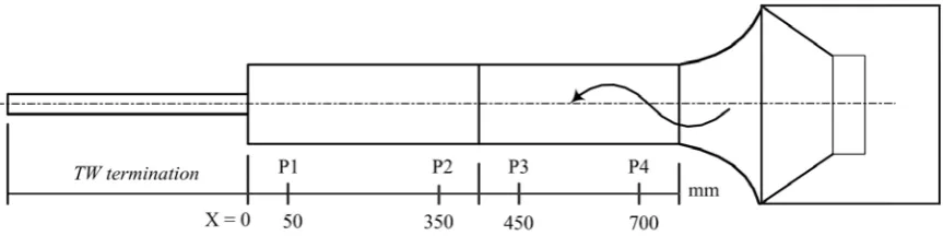
The jet pump sample used for this experiment is a single hole 7° jet pump with orientation as depicted in Figure 2.15 (other jet pump samples are introduced in Chapter 3.1). The closed and traveling wave terminations were chosen to conduct a standing wave and traveling wave inside the setup. The interest of this experiment lies on the phase difference between two pressure sensors at the section after the jet pump (left hand side of Figure 2.15).
35
A pressure amplitude sweep was performed at 113 Hz and the resulting phase difference between sensor P1 and P2 are shown in Figure 2.16.
Figure2.16Phasedifferencebetweensetupwithclosedandtravelingwavetermination.
The phase difference between two pressure sensors separated by 0.3 m for a frequency of 113 Hz is 35.6° for a pure traveling wave. The phase difference for a pure standing wave is zero. From the experimental results, the setup with closed termination results in a phase difference almost zero, thus a standing wave builds up in the setup. The setup with traveling wave termination gives phase difference higher than 30° for pressure amplitude of 100 Pa. This indicates that almost a pure traveling wave builds up in the setup.
Second remark from Figure 2.16 is the decreasing phase difference at higher amplitude for the setup with traveling wave termination. This behavior is in accordance with the result of pressure amplitude sweep for empty setup (Figure 2.14). At higher pressure amplitude, the reflection coefficient increases while the phase difference decreases due to nonlinear effects. The higher pressure amplitude leads to more reflected wave in the setup which contributes to add more standing wave component, hence a lower phase difference and higher reflection coefficient.
In conclusion, the traveling wave termination can generate traveling wave with the jet pump mounted in the setup. Nonlinear behavior at high pressure amplitude was observed in terms of reflection coefficient and phase difference. The traveling wave termination works best at 113 Hz with absorption coefficient of 99.9%.
2.3.
Flow
visualization
39
2.3.5.
Illumination
The illumination of the smoke particles is achieved by using an LED lamp. Different positions of the lamp have been investigated to obtain the best contrast of the smoke and the black background. The black background is provided using a black cloth. However, there are some problems that need to be addressed to obtain a good quality of the picture. The first one is the glare caused by the circular wall of the tube. This problem is solved by placing the LED lamp at the end of the open (or closed) setup and thus provides illumination from inside the tube. However, for the traveling wave termination, this lighting position cannot be applied and hence the LED lamp should give illumination from outside of the tube. It was noted that by putting the LED lamp parallel to the tube rotational axis, the tube reflection appears in the picture. Therefore, this configuration should be avoided. Putting the lamp beside the camera also leads to a visible tube reflection. Illuminating the tube from the back gives a better result and the lamp should be placed in an angle with respect to the tube axis (Figure 2.20).
Figure2.19Schematicdrawingofthelightingpositionforstandingwavesetup(upperview,nottoscale).
40
The second problem is the low contrast between the smoke and the black background. The black cloth can also reflect light and therefore all the light inside the room should be switched off except the LED lamp. The best contrast is achieved in an open and closed end setup because the black cloth is located far away from the LED lamp, consequently only little reflection comes from the background. On the other hand, the setup with traveling wave termination cannot have as black background as the open and closed setup.
The fluid selection also contributes to improve the contrast of the picture, thus the Safex smoke liquid is used for further experiments.
2.3.6.
High
‐
speed
camera
A high‐speed camera is used to capture the movement of the gas inside the setup. A Phantom v7.3 high‐speed camera with a Nikkor 40 mm Macro lens at aperture f/3.6 is used for the flow visualization. The high‐speed camera is set to capture 1000 frame per second, therefore it captures the mean flow at nine points over a period for 113 Hz. Higher frame rate is possible to use (up to 6500 fps), however it requires more light that cannot be done with conventional lighting.
2.4.
Summary
42
Based on this experiment, the applicability of the three assumptions is concluded. The discussion on the applicability of the three assumptions is presented in this chapter.
The flow visualization experiment was carried out for one jet pump sample only. This experiment was performed to know whether the smoke wire method is sufficient to capture the flow pattern. If so, this method can be used for future research with other jet pump samples. The obtained flow patterns will also be a reference for flow visualization of other jet pump samples. The flow visualization experiment uses the smoke wire test section described in Chapter 2.3.1.
3.1.
Jet
pump
samples
To conduct the two experiments, four jet pump samples have been designed with varied geometries. In order to design a jet pump, the geometry has to be defined. Figure 3.1 presents the geometry of a jet pump.
Figure3.1Jetpumpgeometry.
Based on the assumption of minor loss coefficient for a steady flow, the minor loss coefficient depends on the narrowest and widest cross‐sectional area of the jet pump opening and the radius of curvature. This narrowest area is defined by the waist radius , while the widest is defined by the radius . The opening near the jet pump waist is rounded with a curvature of . These parameters are kept constant for all jet pump samples while varying the number of holes and the taper angle . The taper angle and the cross‐sectional area determines the length of the jet pump .
49
3.3.1.
Pressure
and
power
measurement
The pressure and power measurement was conducted for all jet pump samples. The effect of the taper angle, the number of holes and the jet pump termination on the time‐averaged pressure drop and acoustic power dissipation are explained. The experimental minor loss coefficients for oscillating flow, forward flow and backward flow are determined from this experiment. The discussion on the applicability of the three assumptions is also presented in this chapter.
3.3.1.1.
Effect
of
taper
angle
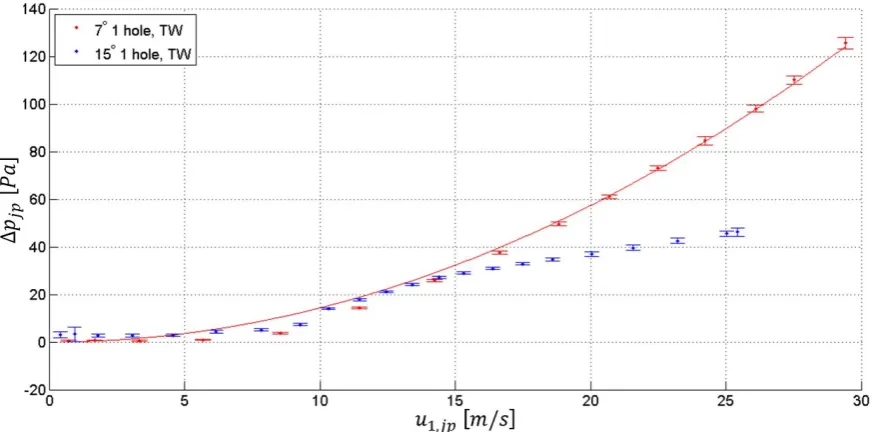
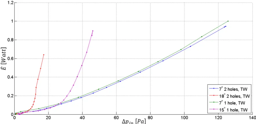
The effect of the taper angle on the pressure drop is presented in Figure 3.3 for the case of a single hole jet pump with quadratic fit for the 7° jet pumps. Figure 3.3 shows the pressure drop as a function of velocity amplitude with vertical error bar for each data point. The vertical error bar is obtained from the measurement over two minutes for one velocity amplitude. Only the results of experiments with the traveling wave termination are shown here. For the results of other terminations, readers are referred to Appendix B. The double hole jet pumps are not shown in this figure because they generate the same trends.
Figure3.3Effectoftaperangleonpressuredrop.
Two samples are compared: the 7° and 15° taper angle for single hole jet pump. From Figure 3.3, it is shown that higher taper angle result in a lower pressure drop. A quadratic curve fitting was done to the results of 7° jet pump according to Backhaus and Swift model (Equation (3.1)). It can be seen that the curve fitting match the results at high pressure amplitude. However, for the 15° jet pump, the experimental result reveals that this sample does not behave quadratically.
50
higher taper angle leads to higher power dissipation for both single and double hole jet pumps. Thus, the assumption on Backhaus and Swift model for energy dissipation holds for all cases.
Figure3.4Pressuredropcurvefor15°and18°jetpump.
Figure3.5Effectoftaperangleonpowerdissipation.
From the quadratic fit of the pressure drop curve, the minor loss coefficient can be determined. The discussion on the estimated minor loss coefficient will be presented later in Chapter 3.3.1.4.
51
of the pipe (see Figure 3.6). The pressure drop and the energy dissipation over the orifice depend on the cross‐sectional area of the vena contracta [23]. The area of the vena contracta depends on the curvature of the junction, i.e. the rounded edge gives larger , hence smaller pressure drop.
Figure3.6Formationofavenacontractainacontraction[23].
The flow separation can also occur in the case of expansion, such as in a diffuser. Idel’chik [31] has studied the minor loss coefficient for steady flow in a diffuser extensively. A nonuniform velocity distribution is generally formed in the stretch before a sudden expansion. This has a strong effect on the actual pressure losses and considerably increases them above the values calculated from the Borda‐Carnot formula [31].
Figure3.7Velocityprofileinadiffuser[31].
A more severe flow separation can occur in a diffuser with taper angle higher than 10° [31]. As depicted in Figure 3.8, there is a region where the flow turns to reverse direction, thus creating a zone with recirculation. This phenomenon may occur for the 15° and 18° jet pumps.
(a) Velocity profile (b) Formation of eddies
53
(a) Forward flow: no formation of vena contracta.
(a) Backward flow: due to the contraction at jet pump waist, vena contracta is formed.
Figure3.10Illustrationofvenacontractaformationinajetpump.
The energy dissipation behavior can also be explained by looking at Figure 3.9. Case B
results in a higher and consequently, higher power dissipation. This is in
accordance with the experimental results, i.e. higher taper angle jet pumps result in higher power dissipation.
From the results of pressure drop and power dissipation measurement, it is highly possible that case B occurs. The minor loss coefficient for backward flow is higher than what is predicted by the assumption on steady flow minor loss coefficient. This hypothesis will be confirmed later by estimating the value of and from the experiment. The calculation of the experimental and and the discussion will be presented in Chapter 3.3.1.4.
3.3.1.2.
Effect
of
number
of
holes
According to the assumption on the minor loss coefficient for steady flow, the minor loss coefficient for expansion only depends on the widest and narrowest cross‐sectional area of the jet pump, while the minor loss coefficient for contraction depends on the edge of the jet pump hole, i.e. sharp or rounded edge. Based on this assumption, the single hole and double hole jet pump should have the same pressure drop. However, the experimental results show discrepancy between the two jet pump samples. Figure 3.11 and Figure 3.12 present the effect of the number of holes. Both the pressure drop and power dissipation increases with increasing number of holes. These results suggest that the assumption on minor loss coefficient for steady flow cannot be used for oscillatory flow.
54
Carnot formula, the tabulated values, or both that are not applicable to the case of oscillatory flow.
Figure3.11Effectofnumberofholesonpressuredrop.
The double hole 7° jet pump gives a higher pressure drop. The curve fit based on Equation (3.1) matches the experimental data at high pressure amplitude.
Figure3.12Effectofnumberofholesonpowerdissipation.
The double hole 7° jet pump gives a higher pressure drop. The curve fit based on Equation (3.12) matches the experimental data.
56
Regardless of the analysis of case (a) and (b), it is evident that the assumption on minor loss coefficient for steady flow cannot be applied to this experiment.
The higher power dissipation for the double hole jet pump is investigated. Energy dissipation could be caused by turbulence effects [32]. Therefore, the critical Reynolds number of the flow is calculated, and consequently, the velocity amplitude at which the flow starts to become turbulent is determined. The transition between laminar and turbulent in oscillating flow depends on the dimensionless frequency [39]. The dimensionless frequency is defined in Equation (3.15).
(3.15)
where is kinematic viscosity and is the tube radius, in this case , . In our case where 7, the critical Reynolds number is:
, 882√ (3.16)
The Reynolds number of an oscillating flow can be calculated in the same way with steady flow, thus it depends on the velocity amplitude. The velocity amplitude at which the transition between laminar and turbulent flow occur is found to be higher than 45 m/s for all jet pump samples. Since all experiments are conducted at velocity amplitude lower than 40 m/s, the flow is laminar. However, the laminar flow can still conduct higher energy dissipation due to the effect of the coupling of two jet streams.
The coupling of two parallel jet streams in a steady airflow has been studied by Nasr and Lai [32]. They show that a recirculating zone exists in between the two jets and the velocity profile is presented in Figure 3.13.
Figure3.13Schematicdiagramoftwoparalleljetstreams[32].
57
is zero. The two jets continue to merge in this region until they are combined as a single jet flow. The starting point of the combined region is indicated by the combined point where the velocity on the axis reaches its maximum value.
The recirculation zone could lead to higher energy dissipation due to the turbulence activities [32]. Nasr and Lai compare the effect of two parallel jets and single jets. It was found that the turbulence activities in the recirculation zone and the interaction of recirculating flow with the inner shear layer are significantly stronger for the two parallel jets than for the single jet. This may lead to complex flow structures as suggested by Huang and Tsai [33]. In their experiments of visualization of a swirling double concentric jet flow, the flow field in the recirculating zone is characterized by complex flow structures such as dual rings, vortex breakdown, and vortex shedding [33]. Thus, it is necessary to perform the flow visualization for the double hole jet pumps to know whether complex flow patterns are formed and whether this case causes higher energy dissipation. However, this case is not covered in this thesis and is left for future research.
In conclusion, the assumption on minor loss coefficient for steady flow cannot be applied for an oscillatory flow. This hypothesis will be confirmed later by calculating the experimental minor loss coefficient (Chapter 3.3.1.4). However, this analysis is only valid if Iguchi hypothesis holds. This argument remains as a hypothesis since the steady flow measurement was not performed in this thesis. Thus, it is necessary to perform the steady flow measurement to clarify the assumptions that are used for this experiment.
The experimental results on the effect of taper angle and number of holes leads to a hypothesis that the taper angle effects are more dominant than the effects of number of holes. This behavior is clearly observed when the acoustic power dissipation is plotted against the pressure drop (Figure 3.14).
Figure3.14Powerdissipationplottedagainstpressuredrop.
58
3.3.1.3.
Effect
of
wave
phasing
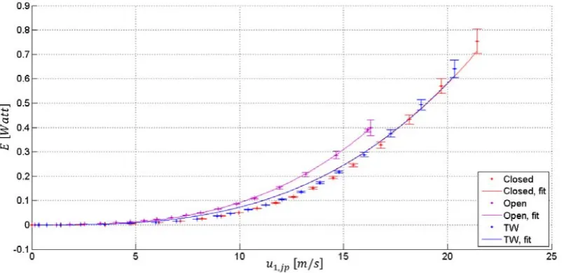
The effect of wave phasing can be seen by performing the experiment using three different terminations. The traveling wave termination creates a traveling wave field inside the setup, thus the phase difference between the pressure and velocity is close to zero. Both open end and closed end creates a standing wave in the main tube, in which the phase difference between the pressure and velocity is close to 90°. The difference between open end and closed end lies on the reflection coefficient: 1 for an ideal setup with closed end and ‐1 for an open end. The negative sign is due to the 180° phase shift between the forward and backward traveling wave.
Figure 3.15 and Figure 3.16 depict the effect of wave phasing in term of pressure drop for the double hole 7° jet pump and 18° jet pump respectively. For other jet pump samples, readers are referred to Appendix B. The results show that different terminations do not give significant effect as the experimental results overlay each other. The only difference lies on the open setup of the 18° jet pump experiment that shows a higher pressure drop.
Figure3.15Effectofwavephasingonpressuredropforlowtaperanglejetpump.
59
Figure3.17Effectofwavephasingonpowerdissipationforthe18°jetpump.
In terms of acoustic power dissipation, the results of the closed setup and the setup with traveling wave termination do not differ significantly. The open end gives higher value for all samples. The discrepancy between the results of open setup and other terminations could be caused by the effectiveness constant. The effectiveness constant could have incorrect scaling as indicated by the velocity amplitude shift in Figure 3.16 and Figure 3.17. The result of the 18° jet pump in as open setup has the same magnitude as the other two cases but with velocity amplitude shifted.
3.3.1.4.
Estimation
of
experimental
minor
loss
coefficients
The estimation of minor loss coefficients for the oscillatory flow, the forward flow and the backward flow was done to check the applicability of the minor loss coefficient for steady flow for oscillatory flow. In Chapter 3.3.1.1, it is suggested that the minor loss coefficient for backward steady flow gives higher deviation than the forward steady flow compared to the experimental result (Case B). In order to check this hypothesis, the values of the experimental minor loss coefficients are determined.
63
0° 45° 90°
135° 180° 225°
270° 315° 360°
Figure3.21Gasoscillation.
Obtained for the single hole 7° jet pump at 113 Hz and velocity amplitude of 10.5 m/s using setup with closed termination.
64
t = 0 s t = 0.044 s
t = 0.079 s t = 0.115 s
t = 0.137 s t = 0.164 s
t = 0.177 s t = 0.181 s
Figure3.22Trailofsmokesuckedintothejetpump.
65
An outburst flow is visible at low velocity amplitude of about 1.5 m/s. The length of the jet flow is about 3 cm from the jet pump opening. This flow was observed 345 s after the first image was taken. The phase angle of the pressure is 348°. However, this kind of outburst flow is not visible at higher velocity amplitude. This may be causes by the high velocity of the outburst flow so that the smoke particles are dispersed rapidly.
Figure3.23Outburstflow.
Obtained for the single hole 7° jet pump at 113 Hz and velocity amplitude of 1.5 m/s using setup with traveling wave termination.
Two flow patterns and the gas oscillation are visible during the flow visualization experiment. The utilization of the high speed camera also gives contribution to capture the gas oscillation and more detailed evolution of the flow pattern over a short period of time. In conclusion, the smoke wire method can be used for further research to obtain the flow pattern generated by a jet pump in oscillatory flow.
3.3.2.2.
Vortex
detection
and
propagation
speed
calculation
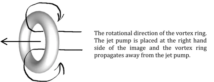
The flow visualization was performed at 28, 56, 80 and 169 Hz with fixed velocity amplitude of 13, 13.5, 17 and 16 m/s respectively. From this experiment, a vortex ring propagates away from the jet pump is visible. The propagation of the vortex ring is visible if the captured frames are shown in sequence as a video recording such that the successive movement of the vortex ring can be distinguished. If one looks into one captured frame only, the vortex ring is indistinguishable from the surrounding. The vortex ring is visible in the recording as a black line moving away from the jet pump hole only when there is a large amount of smoke in the test section. Due to the position of the smoke wire at the downstream of the jet pump, the vortex ring cannot be captured as a ring of smoke propagating away from the jet pump opening.
67
t = 0.209 s t = 0.210 s t = 0.213 s t = 0.214 s
t = 0.215 s t = 0.216 s t = 0.217 s t = 0.218 s
Figure3.25Vortexedgedetection.
Obtained for the single hole 7° jet pump at 80 Hz and velocity amplitude of 10.5 m/s.
The vortex propagation speed is determined by manually measuring the distance traveled by the vortex over a certain time. The pictures used for this measurement is the original picture without any image processing. The vortex propagation speed is expressed in Equation (3.17).
(3.17)
69
and Swift model does not hold for high taper angle jet pump. The second assumption on the theoretical value of minor loss coefficient for expansion and contraction also fails, suggesting that the formula and typical values for steady flow cannot be used for oscillatory flow.
75
[38]Swift, G.W. (2002). Thermoacoustic: A unifying perspective for some engines and
refrigerators.Acoustical Society of America.
76
APPENDIX
A
TRAVELING
WAVE
TERMINATION
MODEL
ModelingandValidation
In this section, the parameters that were used in the model and the result obtained by van der Eerden [11] will be presented and compared. Figure 0.1 shows the configuration of two tubes in series and the boundary conditions used by van der Eerden [11].
Figure0.1Atravelingwaveterminationconnectedtothemaintubeinseries[11].
Standard air conditions were used and the values are listed in Table 0.1.
Table0.1Standardairconditions.
Parameter Unit Value
Specific heat, Cp J/kgC 1006
Mean density, kg/m3 1.22
Dynamic viscosity, Ns/m2 1.82e‐05
Speed of sound, m/s 343.3
Square root of Prandtl number, ‐ 0.845
Ratio of specific heat, ‐ 1.4
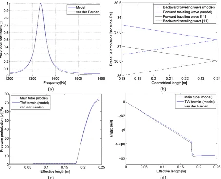
Note that the length Lin Figure 0.1 refers to the geometrical length. Another term that is used in the model is the effective length. The effective length is equal to the geometrical length increased by an end correction and will be explained later. It was obtained by van der Eerden[11] that for such configuration, 100% absorption can be achieved for frequency 1337 Hz. Figure 0.2 shows the absorption coefficient as a function of frequency and the acoustic variables in both tubes.
Lg,2=0.06m
Ri,2=0.005m
Lg,1=0.18m
Ri,1=0.043m
P0=1atm
Maintube
77
(a) (b)
(c) (d)
Figure0.2ComparisonofmodelimplementationandvanderEerden’sresult[11]: (a) sound absorption coefficient as a function of frequency, (b) amplitude of the forward and backward propagating wave in the traveling wave termination, (c) pressure perturbation magnitude and (d) phase
at 1337 Hz. Taken for 0.18 and 0.0636 .
The model implementation shows a good agreement with the reference. Figure 0.2(a) indicates a maximum absorption when the frequency reaches 1337 Hz. At this frequency, it can be seen from Figure 0.2(b) that the forward and backward propagating waves behave similarly. The negative linear gradient shows that there is decay on pressure amplitude of the forward wave, followed by the same decay for the reflective wave. The same gradient of the incident and reflection wave indicates a constant attenuation inside the traveling wave termination as an effect of the wave propagation constant .
Figure 0.2 (c) is also in accordance with Figure 0.2(d), which shows a traveling wave inside the main tube, marked by the constant pressure and the constant phase change. While inside the traveling wave termination, it is shown that there is relatively large pressure amplitude and a constant phase. These behaviors signify that there is a standing wave pattern inside the traveling wave termination.
79
From Figure 0.2 and Figure 0.3, it can be concluded the end correction influences the acoustic field inside the setup. The difference of applying the end correction at both tubes can be seen in Figure 0.2(b) and Figure 0.3. Since the acoustic field inside the setup is influenced by the end correction, it is desired to know whether it can influence the working frequency as well. Thus, the following test was performed.
The model was run to obtain the working frequency for three different scenarios: (1) uncorrected length, (2) end correction applied at the traveling wave termination, and (3) end correction applied at the traveling wave termination and the main tube. The results are depicted in Figure 0.4. It can be seen that using the uncorrected length results in a higher working frequency than the corrected length. The end correction of the main tube does not give significant effect on the working frequency compared to the end correction of the traveling wave termination, as these two graphs overlay each other. This result is in accordance with the one obtained by van der Eerden [11]. Thus, it can be concluded that the end correction applied for both tubes does not give significant influence on the working frequency, but it influences the pressure amplitude at the traveling wave termination, as shown by Figure 0.2(b) and Figure 0.3.
Figure0.4Influenceofendcorrection.
Using the geometrical length , and the effective length , as an input for the model,
the outcomes in Section 2.2.3 and 2.2.4 are obtained.
Thetravelingwaveterminationmodel
80
Figure0.5Relationbetweentuberadius,length,absorptioncoefficientandworkingfrequency.
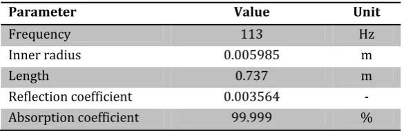
Figure 0.5shows that in order to obtain the working frequency at 100 Hz (maxima point at 100 Hz), it is favorable to have a tube radius larger than 6 mm. For working frequency of 100 Hz, a tube inner diameter of 6,1 mm should be used. However, the ordered tube arrived with inner diameter of 5.985 mm. According to Figure 0.5, this tube is suitable for a working frequency of 113 Hz. Nevertheless, this tube can also be used for 100 Hz with absorption coefficient of 99.9% if one uses a length of 85 cm. Since there is a limitation on the length of the tube, the 113 Hz was chosen for resonator length of 0.737 m.
Experimentwithfoams
To improve the absorption coefficient at 113 Hz, two kinds of porous material are attached to the junction of the traveling wave termination. This was done based on the presumption that higher reflection coefficient than the model might result because the flow is not purely a one‐ dimensional flow. Therefore, it is desired to have a flow only in one direction to see whether this behavior keeps appearing. This reason is motivated by the fact that the resonator model is a one‐dimensional model. The velocity in radial direction is assumed to be zero, therefore this model predicts only one‐dimensional flow. Hence, the porous materials are expected to act as a flow straightener and the experimental results are expected to match better with the model.
The porous materials are attached to the junction of the main tube and the traveling wave termination, where it covers the entire surface of the end wall of the main tube and the entrance hole to the traveling wave termination. The frequency sweep is performed at 100 Pa and 600 Pa. The comparison of the experimental results is presented in Figure 0.6.
81
(a) Foam sample (b) Glass wool sample
(c) Frequency sweep at 100 Pa (d) Frequency sweep at 600 Pa
Figure0.6Thecomparisonoffoameffectat100Paand600Pa.
It was expected that the porous materials should give results that match better with the model, however this does not happen. As can be seen around 113 Hz, both samples result in a higher reflection coefficient compared to the experiments without porous material. This might be caused by the location where the samples are attached, which covers the entire surface of the end wall of the main tube. Due to the random structure of the sample matrix, the end wall of the main tube generates an absorbed backward travelling wave (Figure 0.7). The phase of the absorbed backward traveling wave cannot be predicted because of the sample structure, hence it is possible that this backward wave is not in accordance with the initial design. On the other hand, the end wall of the traveling wave termination still has a reflecting surface that produces the same reflection wave. Thus, the two reflection waves from both traveling wave termination and the main tube will not be able to cancel each other as good as the case when the porous material is not used.
(a) Without porous material (b) With porous material
Figure0.7Schematicofthebackwardtravelingwave.
82
From this set of experiment, it can be concluded that the porous material does not improve the performance of the traveling wave termination. This means that either the foam does not act as a flow straightener, or it acts as a flow straightener but there is other parameter that affects the performance of the traveling wave termination. One way to check whether the porous material can act as a flow straightener is by attaching the foam only at the hole to the entrance of the traveling wave termination, and see whether the result match better with the model.
83
APPENDIX
B
EXPERIMENTAL
RESULTS
OF
PRESSURE
AND
POWER
MEASUREMENT
86 COP
88
REVERSEDJETPUMP
92
APPENDIX
C
CALCULATION
OF
INNER
WALL
SURFACE
AREA
The calculation of the inner wall surface area was performed for all jet pump samples. The dimensions are known from measurement and are listed in Table 3.1. The inner wall surface area is defined as the area of the tapered surface and the curved surface that connects the taper
and , . Since the radius of curvature cannot be measured, it was assumed to be 5 mm
and that the curvature forms an exact circle. The area that contributes to the calculation of the inner wall surface area is depicted in Figure 0.1 with red line.
Figure0.1Innerwallsurfacearea
The tapered surface area is defined in the following equation.
(B.1) Substituting , , and with Equation (B.2), can be written as a function of , , and .
sin
, tan
(B.2)
93
The curved surface area can be calculated based on the parametric formulation for a circle equation with its center is located in (h,k) in Cartesian coordinate and a radius . This parametric equation can be expressed by Equation (B.3).
sin (B.3)
cos
Assuming the origin (0,0) is located in point O (see Figure 0.1), Equation (B.3) can be expressed as follows:
sin
(B.4)
, cos
The curvature in Figure 0.1 is symmetric to the axis. The surface area of the curvature if it is rotated with respect to the axis is formulated in Equation (B.5).
2 (B.5)
With is defined in the following equation.
(B.6)
Deriving Equation (B.4) with respect to , the following equation is obtained.
(B.7) Therefore, Equation (B.5) can be written as follows:
2 , cos (B.8)
94
APPENDIX
D
SEQUENCE
OF
IMAGES
FROM
FLOW
VISUALIZATION
Vortex ring propagation
t = 0.209 s t = 0.210 s t = 0.211 s t = 0.212 s
t = 0.213 s t = 0.214 s t = 0.215 s t = 0.216 s