Relational Algebra and SQL Query Visualisation

Relational Algebra and SQL

Query Visualisation

Giorgos Constantinou

[email protected]

Supervisor: Dr. Peter McBrien

Second Marker: Dr. Natasa Przulj

Abstract

Relational algebra and the industry standard SQL are core topic covered in un-dergraduate database courses. Database management systems translate SQL state-ments into a procedural query plan composed with operations similar to those that arise in relational algebra. Learning relational algebra makes students familiar with this process. Moreover they understand the difference between procedural and declarative query languages. Students that understand the relation between the two languages have the required knowledge to query databases. Additionally, it is equally important to appreciate the difference in expressiveness of the two languages and that SQL is a superset of relational algebra.

Currently there is no tool that can execute both types of queries and show the relation of the two in terms of the execution process. As a result students exercise on the two languages independently and do not acquire crucial knowledge which is useful in constructing optimised queries. Moreover, the available tools that support relational algebra fail to show the difference between basic and derived operations and students do not appreciate the simplicity of the evaluation process.

In this report we introduce Query Visualiser (QV), a tool that facilitates the learning process of both languages. Using extended relational algebra, SQL queries are translated into a procedural query plan. This tool provides transparency to the evaluation process by illustrating the results using a tree hosting intermediate results of the evaluation. The tree is constructed with operations that arise in relational algebra or in the extended one in an attempt to show their relations. In addition, the system can perform simple optimisations and see how they affect the performance using the analytical statistics of the evaluation. Also, the user can dynamically define new derived operators and see how they are converted and executed using basic operations.

Acknowledgments

I would first like to thank my supervisor, Dr. Peter McBrien for his valuable feedback and support during the course of the project. His critical reviews and guidelines always motivated me to carry on.

Finally I want to thank my friends and family for their endless patience through-out my time at Imperial College.

Contents

2.2 Relational Algebra . . . 13

2.3 SQL . . . 16

2.4 Query Execution . . . 16

2.4.1 Extended Relational Algebra . . . 17

2.4.2 Translations . . . 18 2.4.3 Intermediate results . . . 19 2.4.4 Data lineage . . . 20 2.5 Relevant Technologies . . . 20 2.6 Related Work . . . 21 2.6.1 WinRDBI . . . 21 2.6.2 iDFQL . . . 22 2.6.3 RELATIONAL . . . 23 2.6.4 RALT . . . 24

2.6.5 Aqua Data Studio . . . 25

2.6.6 Features Comparison . . . 25

3 System Architecture 27 3.1 View Layer . . . 27

3.2 Controlling Layer . . . 27

3.3 Model Layer . . . 29

4 Query Representation and Execution 30 4.1 Query Syntax . . . 30

4.1.2 ERA Syntax . . . 31

4.1.3 SQL Syntax . . . 32

4.1.4 Syntax Errors . . . 32

4.2 Query Tree . . . 32

4.3 Query Evaluation . . . 33

4.3.1 General Evaluation Module . . . 33

4.3.2 Specialist Evaluation Modules . . . 33

4.3.3 Evaluation Errors . . . 35

4.3.4 Views . . . 36

4.3.5 Execution Statistics . . . 37

4.3.6 Data Lineage . . . 39

4.4 Algebra Optimisation . . . 40

4.4.1 Unary Input Case . . . 40

4.4.2 Binary Input Case . . . 41

5 Workspace and Visualisers 42 5.1 Relation Explorer . . . 43 5.2 Import . . . 43 5.3 Tab Containers . . . 44 5.4 Query Panel . . . 45 5.5 Query Editor . . . 45 5.6 Result Visualisers . . . 47 5.6.1 Data Grid . . . 47 5.6.2 Intermediate Results . . . 48 5.6.3 Chart . . . 50 5.6.4 Console . . . 51 5.6.5 Execution Cost . . . 51 5.7 Visual Optimiser . . . 52

5.7.1 Tree Execution Time . . . 54

5.7.2 Tree Maximum Memory Usage . . . 54

5.7.3 Operation Nodes Execution Time . . . 54

5.7.4 Operation Memory Usage . . . 55

6 Implementation Details 56 6.1 Overview . . . 56

6.2 Graphical Interface . . . 57

6.3 Database Representation . . . 57

6.4 Workspace Persistence . . . 58

6.5 Query Tree Representation . . . 58

6.6 Parsers . . . 58

6.8 Dynamic Operator Construction . . . 60

6.9 Mono and multi-platform compatibility . . . 61

6.10 Third-party Modules . . . 61

6.10.1 Text Editor . . . 61

6.10.2 Drawing Charts . . . 63

6.11 Creating ERA Trees from SQL . . . 63

6.12 Extending QV . . . 63

6.12.1 Extending the existing languages . . . 64

6.12.2 Introducing a new query language . . . 65

7 Correctness and Stability 67 7.1 Experiments . . . 67 7.1.1 Unit testing . . . 67 7.1.2 Stress Testing . . . 68 7.2 Results . . . 68 7.3 Analysis . . . 69 8 Usability Experiments 70 8.1 End-User Test . . . 70 8.1.1 End-user profiles . . . 70 8.1.2 Exercise Sheet . . . 71 8.1.3 Questionnaire . . . 73 8.1.4 Results . . . 73 8.1.5 Analysis . . . 74

8.2 Nielsen’s Usability Heuristics . . . 75

9 Conclusion 79 9.1 Achievements and contributions . . . 79

9.2 Future Work . . . 80

Bibliography 80

A QV Details 83

B Tutorial Solutions 87

Chapter 1

Introduction

1.1

Motivation

Relational databases are the core of the introductory and advanced database courses. Most of these courses cover formal query languages such as the relational algebra (RA) and Structured Query Language (SQL). It is difficult for students to decide whether queries written on paper are correct or not. Alternatively it is much easier to do so using trial and error on a system capable of evaluating such queries.

Almost all of today’s database management systems support SQL. They trans-late declarative queries into lower-level operations similar to the RA operations. It is important for the students to familiarise with this concept in order to get a better understanding on how the two querying languages are related. One of the most im-portant properties of relational algebra and algebra in general is that each operation performed provides a result that can become the input to another operation. Typi-cal queries that students are asked to construct are made up of multiple operations that can be visualised as a tree where operations are evaluated starting from the bottom. Complex queries are usually hard to form and understand and visualising the intermediate result of nodes is helpful. Currently most of the teaching tools that support relational algebra lack the ability to give feedback to the user in order to help in constructing queries. Others provide some feedback using intermediate results but they fail in relating SQL to RA which is crucial in helping the user write optimised SQL queries and often results in unoptimised queries due to lack of appreciating the relation between declarative query evaluation with the relational algebra operations.

1.2

Objectives

We present QV - Query Visualiser, a tool that facilitates the learning of RA and SQL using detailed explanation of the query execution process.. Here we outline the main objectives.

• Building a database - The user should can construct a database using the graphical interface which allows schema and data manipulation.

• Database import - As an alternative to manually constructing a database, the user can provide connection setting for an existing database from where QV imports the data into the workspace.

• Query Syntax- We design and implement a parser for a suitable syntax for relational algebra (RA) and extended relational algebra (ERA). In addition we will implement a parser for the select and set operation statements of SQL.

• Query Evaluation- Evaluate queries written in RA, ERA and SQL. The RA language evaluates all the basic operations. The ERA evaluation inherits the operations of RA and also includes other operations which provide semantic completeness for SQL. The SQL evaluation translates the SQL into a tree of ERA operations which can then be evaluated with the ERA evaluator.

• Error Reporting - To help the user debug queries useful feedback is provided in case of errors. It should be clear whether errors are due to syntax or evaluation reasons. Line and position of the error in the query are also provided where appropriate.

• Intermediate Results - When evaluating the query we temporarily store the intermediate results of all the operators applied and present them in a tree that represents the evaluation process. The user can navigate the tree and analyse step by step how the query was evaluated.

• Dynamic Operators - The user can define new relational algebra operators, ranging from simple operators like set intersection to complex operators like

division. After evaluation the user can browse the intermediate results and see how the new derived operator was dynamically converted into basic relational algebra operations.

• Data Lineage - From the result the user can select rows and see at all nodes in the intermediate results tree what data contributed to the result. This will be indicated by highlighting the respective rows of the nodes.

• Execution Statistics- Timing and memory usage statistics will be provided in order for the user to understand the complexity level of queries.

• Query Optimisation - The system will be able to modify evaluation trees in order to optimise the performance. The user will see step by step this modifications and statistics on how each one affects the performance.

1.3

Report Structure

The report is structured into the following chapters:

• BackgroundIn this chapter we discuss the fundamentals of relational database models and formal query languages and investigate relevant technologies. We then look at different designs and implementations of tools relevant to our goal and we conclude with a comparison of their features.

The next three chapters cover the specification and the design of a tool that meets the objectives in Section 1.2.

• System Architecture We outline the modules of the system and we describe their respective tasks along with a description on how different modules of the system are related and their dependencies.

• Query Representation and Execution We specify a suitable syntax for the query languages and their semantics. We provide a description of an intermediate representation of queries using syntactical trees. Also in this chapter there is a description on how to perform data lineage, simple query optimisations and calculate statistics on execution performance.

• Workspace and VisualisersAfter we specified the evaluation process of the system in the previous chapter we describe the user interface and how the user can manipulate the database model and execute queries. We show the different methods of showing the evaluation results and described how data lineage is displayed.

• Implementation DetailsBased on the design we documented in the previous chapters we describe the important implementation details of QV

The next two chapters cover the evaluation of the implemented system

• Correctness and StabilityThis chapter is concerned with quantitative tests on the implemented system.

• Usability Experiment We evaluate the performance of the system by per-forming an experiment with a set of end-users and we discuss the outcome.

• Conclusion This chapter concludes the report by recognising the areas of success and failure and suggesting future extensions.

Chapter 2

Background

2.1

Relational Data Model

Introduced by E.F Codd[5] along with the relational algebra and it is the most common data model used for databases.

In a relational model a relation consist of a heading(set of attributes) and a body(set of tuples) that represents the relation value. Thedegreeof a relation refers to the number of attribute in the relation header and the cardinality of a relation refers to the number of tuples in the relation body (value). AnAttributeis formed by the attribute name and the domain (type) and a tuple is a set of zero or more attribute values that conform to the relation header.

There are two Relation Classes which are classified as base relations and de-rived relations (views):

• Base Relations are defines by the data tuples that represent the relation value. In relational model implementations base relations are defined using a Data Definition Language(DDL) such an example is SQL which uses tables to represent base relations 1_.

• Derived Relations(Views) are the result of applying relational operations on one or more relations.

2.2

Relational Algebra

Relational algebra is a procedural language based on algebraic concepts. Codd sug-gested a modification of the mathematical approach and defined the term ‘relational

algebra’. It essentially consists of a collection of operators that take as input re-lations and produce rere-lations as result. Since both the operands and the results are relations, expressions can be nested in RA as in any algebraic expression. Also because relations are sets all the usual set operators such as union can be used. In addition to the set operators other operators such as select2 and join are used.

Basic Operators

RA relies only on five primitive operators proposed by Codd (Selection, Projection, Product, Union, Difference), which make RA a relationally complete query language. In addition to these operators, the rename operator (ρ) is also treated as primitive with the introduction of ISBL 3.

Operator Description Project

πA1,...,An(R)

Returns tuples from R that can be defined as the set that is ob-tained when all the tuples in R are restricted to {A1, ..., An}

Select σC(R)

Generalised Selection returns tuples from relation R that satisfy C which is a propositional formula of atoms allowed in Normal Selection and the logical operators and (∧), or (∨) and negation (¬).

Normal selection αθβ orαθV where: α, β are attributes of relation R.

θ is a binary set operator {=,6=, <,≤, >,≥}. V is a value constant.

Cartesian Product R×S

Cartesian Product returns tuples from all the possible combina-tions of R and S tuples. GivenR and S have n and m attributes the result will hold tuples of n+m attributes

Union R∪S

Returns all the tuples from R and S . The two relations R and S must beunion compatible

Difference R−S

Returns all the tuples from R that do not appear in S . The two relations R and S must be union compatible.

Rename ρA/B(R)

Returns an identical result to R except that in all tuples attribute A is renamed to B

Table 2.1: Relational Algebra Primitive Operators

2_{Also called restriction. Not to be confused with SQL SELECT.}

3_{Information Systems Base Language: One of the earliest database management systems to}

Derived Operators

A range of operators are available which derive from the primitive ones. Operator Description

Intersection

R∩S≡R−(R−S)

Returns the common tuples from R and S . The two relations R and S must beunion compatible.

Theta Join

R./θ S≡σθ(R×S)

Returns tuples from the Cartesian product which satisfy θ. θ is a predicate aφb where:

a and b are attributes of R and S respectively φ is a comparison operator{=,6=, <,≤, >,≥}

Equijoin is a special type of theta join where φ is always =. Natural Join

R./S≡

πR.∪S(

σR.A1=S.A1...(R×S))

Returns tuples from the Cartesian product where common at-tributes between R and S have the same values and removes du-plicated columns. Usually it is required that there is at least one common attribute, if not then the operator acts only as a Carte-sian product.

Semi Join

R_nS ≡ R ./ πR∩S(S)

Returns the same result as the natural join but the result only contains tuples from relationR.

Table 2.2: Relational Algebra Derived Operators Examples

Useful Equivalences[3]

πx(R∪S)≡πx(R)∪πx(S) (2.7)

σA∧B(R) (R∪S)≡πx(R)∪πx(S) (2.8)

σA∧¬(B)(R)≡σA(R)−σB(R) (2.9)

R ./(S∪T)≡(R ./ S)∪(R ./ T) (2.10)

2.3

SQL

Structured Query Language (SQL) is a declarative language used in many imple-mentations of the relational data model and is a super-set of RA. Since it is as expressive as RA it is also relationally complete. SQL uses tables to represent re-lations and columns to represent attributes. SQL is a Data Definition Language (DDL) and uses commands like CREATE, ALTER, DROP and RENAME to define the database schema. At the same time it acts as a Data Manipulation Language (DML) used to manage data within a schema based on commands like INSERT, DELETE, UPDATE SELECT and UNION. We will not be concerned with data entry with SQL statements therefore we will concentrate on the basic forms of the SELECT and set operation4 _{statements. One of the main differences that we need}

to have in mind is that SQL relations (tables) are bags ormulti-sets and notsets as in the RA.

2.4

Query Execution

There are many implementations and discussions on how RA can and is used as the background of SQL from the early stages[4]. When executing an SQL query it is parsed and translated into a sequence tree. Then the references to tables and columns will be checked against the database to validate their existence. At that point the query is translated into a Query Processor Tree 5 which expresses the initial declarative query in a procedural manner. Since at the core of an RDBMS there is an engine that evaluates these algebraic operations, a modification of the standard RA can be used which can also be used as an alternative query language for multi-sets directly.

4UNION, MINUS, INTERSECT

5_{Optimisation is performed at this point using various optimisers that will make adjustments}

2.4.1

Extended Relational Algebra

In order to evaluate RA expressions in relational data models with multi-set seman-tics the Extended Relational Algebra (ERA) proposed by Paul Grefen and Rolf By[8] can be used. The first thing to note is that in ERA, sets are treated as multi-sets. All the standard RA operators have the same definitions except that the duplicates are not removed. The interest is only in the available operators and therefore their formal definitions are omitted from this report.

Generalised Projection

πF1,...,F N(R) (2.11)

It extends the projection operator and permits the use of arithmetic functions. Example

πemployee_name,(current_salary−previous_salary)(Employees)

The operation will return the difference between the new and previous salary of each employee. Note that duplicates will not be removed.

Aggregate Functions

CN Ta(R) (2.12)

Counts the number of instances of attributea

SU Ma(R) (2.13)

Calculates the sum of all values of attribute a from all rows.

M INa(R) (2.14)

Returns the minimum value of attribute a from all rows.

M AXa(R) (2.15)

Returns the maximum value of attributea from all rows.

AV Ga(R)≡

SU Ma(R)

CN Ta(R)

(2.16) Returns the average value of all value of attribute a from all rows.

Unique

δ(R) (2.17)

Removes the duplicated rows from the result of R (converts a bag to a set).

Group By

G1,...,GnΓF1A₁,...,F kAk(R) (2.18)

Aggregates the result by partitioning the tuples based on common attributes G. The other attributes returned are the results of aggregate functionsF on attributes A.

Example

departmentΓCN Temployee_name(Employees)

The Operation will return the number of employees in each department.

Outer Join

(R) [(LEF T|RIGHT) +OU T ER J OIN]C(S) (2.19)

Behave like normal joins in RA but the OUTER token indicates that unmatched columns from the left and/or right accordingly should be matched with NULL values and be part of the result.

2.4.2

Translations

Instead of using basic RA or SQL we will be using ERA for evaluating queries. Note that we can convert RA expressions to ERA using the unique expression δ or by telling the evaluator to use set based semantics. Here are a few SQL statements and there respective ERA equivalents:

Select Statements SELECT A1,...,A3

FROM R1,...Rk

WHERE C1 AND...AND Cm

−−−−−−→πA1,...,An(σC1,...,CmR1×...,×Rk)

If we use the DISTINCT token in the SELECT clause the ERA expression will need to contain theδ operator either before or immediately after the projection.

When the FROM expression contains a JOIN6 _{we can translate it using the RA}

Cartesian product and join7 and vice-versa SELECT A1,...,An

FROM R1JOINRk

ON C1AND...ANDCN

−−→πA1,...,An(R1 ./C1∧...∧CN R2)

In an SQL statement it is often the case that relation are joined using the WHERE clause by equality check on columns from the two tables to be joined. When translating a query we can identify these cases and treat them as the basic join case or vice-versa. Even if additional conditions are specified, this is still prac-tical since the the result of one operation can become the input of another.

SELECT A1,...,An FROM R,S WHERE R.A=S.A AND R.N =S.N AND R.X > V

−→πA1,...,An(σR.X>V∧R.A=S.A∧R.N=S.N(R1×R2))

≡σR.X>V (πA1,...,An(R1 ./R.A=S.A∧R.N=S.N R2))

Set Operations

(SELECT_STATEMENT1)

U N ION|EXCEP T|IN T ERSECT (SELECT_STATEMENT2) −−→ UNION case: δ(R₁ ∪R2) EXCEPT case: δ(R1−R) INTERSECTION case: δ(R1∩R) ≡δ(R₁−(R1−R2))

The set operators provided by SQL require their two parameter relations(tables) to be union compatible like RA. Also the set operators result has no duplicates and is the same as with RA. You can specify using ALL that duplicates should be returned and the respective ERA expression will not be encapsulated byδ.

2.4.3

Intermediate results

When executing the query a syntax tree with ERA operations can be created. This tree can be evaluated starting from the leaf nodes until the head node is reached

6_{NATURAL JOIN, JOIN, LEFT JOIN, RIGHT JOIN, LEFT OUTER JOIN or RIGHT}

OUTER JOIN

7_./,

which is the result of the query. At each step of the evaluation the result of each of these operations is an intermediate result.

2.4.4

Data lineage

Data lineage is an effective method for understanding from where a particular value in a query result was derived and at the same time it can show the source of er-ror when the query result is wrong. Such a feature is valuable in understanding key concepts around both the RA and SQL. Many different approaches exist that successfully implement data lineage and each one has a different cost. One way of achieving this is through meta data attached to the result tuples in order to retrieve the source of the data. This is a complex method and is used for lineage at the schema level and not the data. An alternative method is to store all the interme-diate results of the execution and by applying the inverse of the operations used to produce the result, traverse the execution tree backwards in order to find the sources.

2.5

Relevant Technologies

For the development of an interactive learning tool there is a clear need of an object oriented language that is cross platform compatible, has useful data structures for the application and there is a good GUI library that can be used. The two main alternatives for these purposes are Java and .NET C#.

Java is highly portable and can run on almost all platforms but it’s GUI library

Swing has been around for more that a decade and the available controls need a lot of customisation in order to provide the user with a decent interactive environment. Microsoft C# on .NET Framework offers a lot of data structures such as

DataTablesandDictionariesthat can be proved useful and cutoff a lot of developing hours. The biggest benefit of .NET is that it offers an easy to use GUI toolkit that can produce professional results that maintain the standards of commercial applications. Although until recently .NET was considered only for applications targeting Microsoft Windows systems, an open source implementations of .NET, Mono has been developed and it can perfectly simulate the .NET framework on Microsoft Windows, Linux and Mac OS X. The main restriction is that the developer must not make system calls that will not work on different platforms(E.g. Do not call win32 functions since they are only available in Windows).

2.6

Related Work

In this section we investigate relevant proposed and implemented tools. We discuss their strengths and weaknesses and compare their features in an attempt to outline what our system will inherit and how it compares to them.

2.6.1

WinRDBI

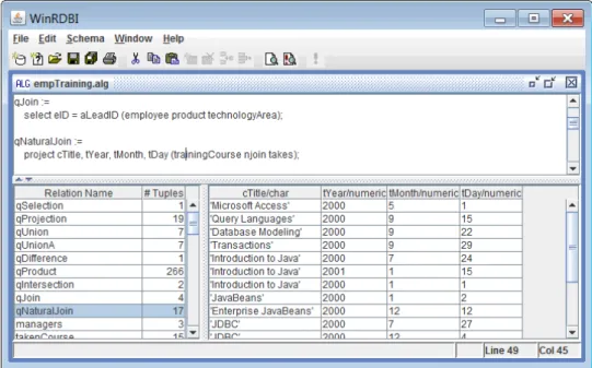
WinRDBI[7] is a graphical interface for RDBI[1] which is written in Prolog and it evaluates queries in relational algebra, domain relational calculus, tuple relational calculus and SQL. It is a Windows tool developed in Visual Basic and it uses the Relation/Tuple notation for the database schema.The interface of the system is split into 3 areas:

1. TheQuery Definition Panel where user can input an SQL or RA query in a simple text editor.

2. TheQuery Result Panelwhere the result of the executed query is presented on a grid.

3. TheDatabase Browser which includes a list of the available relations and a grid that displays the body (data tuples) of the currently selected relation.

To alter the definition of a relations there is a property window that will let you configure the relation attributes and their types. Same properties window is used to create new relations. The first version supported adding and removing tuples to a relation from the main menus and the latest release allows direct editing of the grid. One of the nice features is that you can define multiple relations using RA and use each other as operands in other queries. Although this is one of the options it does not support storing these queries as views and you need to include the definitions of all the referenced relation in the same query file. Note that this also limits the relations from being part of the Database Browser and they can not be reused in an SQL query. Another useful feature is the ability to import relations from existing databases using ODBC.

2.6.2

iDFQL

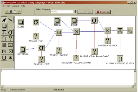
Designed and developed by Appel et al[2]. iDFQL is an interactive environment where you can build RA queries by constructing a diagram that represents relations and operators using a data flow approach. It doesn’t store a data model but instead it connects to a database on which it executes SQL queries to evaluate the RA expression defined in the diagram. The only way of getting data out of the database is by means of a query and there is no support for editing the model. iDFQL facilitate the learning of the relational algebra by showing intermediate results. This is achieved by requesting the result at any node on the diagram.

2.6.3

RELATIONAL

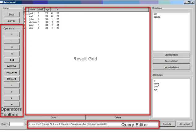
RELATIONAL[15] is a Python application which serves as an educational tool for relational algebra which is available in distributions for Linux, Microsoft Windows and Mac OS X. It provides a simple and easy to navigate graphical interface which allows the user to load/store relations, execute queries on them and show the result as shown in Figure 2.3. Relations are loaded in memory from flat files prior to query execution and can not be edited within the application. The queries are specified in a one line text field using algebraic notation. The operator symbols can not directly be written by the user, instead there is a toolbox with the available operators that will add the corresponding Unicode symbol to the text field. The set of available operators in RELATIONAL extends to advanced operators such as left outer join. Also it provides an option that will apply a simple optimisation by moving the select operations as close to the basic relations as possible. What we found to be a major drawback is the fact that when a query execution fails there is no information for the possible errors and always the same error message "Check your query" is displayed which is not helpful in identifying the source of error.

2.6.4

RALT

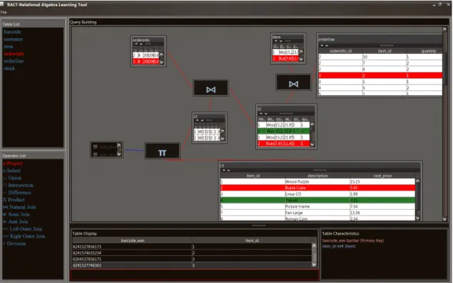
RALT - Relational Algebra Learning Tool [11] is a Java application developed by Pri-tam Mitra which uses an interactive graphical editor for query construction. RALT has an extended set of available operators like RELATIONAL with the addition of

division. The purpose of RALT is to serve as a query visualiser and does not sup-port database editing. There is a panel on the left side of the workspace containing relational algebra operators which can be dragged on to the editor and assist the user in specifying the parameters and the inputs to the operator. This is a defen-sive approach which eliminates the possible syntax errors that arise when writing queries. When the required parameters have been correctly specified the result of the operation is drawn in the editor using a table. This way the user will have im-mediate feedback for every added operator before building th complete query. The query construction is simple and effective but becomes complex for large queries. Also making changes to the query diagram often requires rebuilding large portions of the query again which is time consuming. The unique feature of RALT compared to the other tools is that it shows data lineage. By selecting a row in the result the rows in all the previous nodes that contributed are highlighted to indicate why the selection is part of the result.

2.6.5

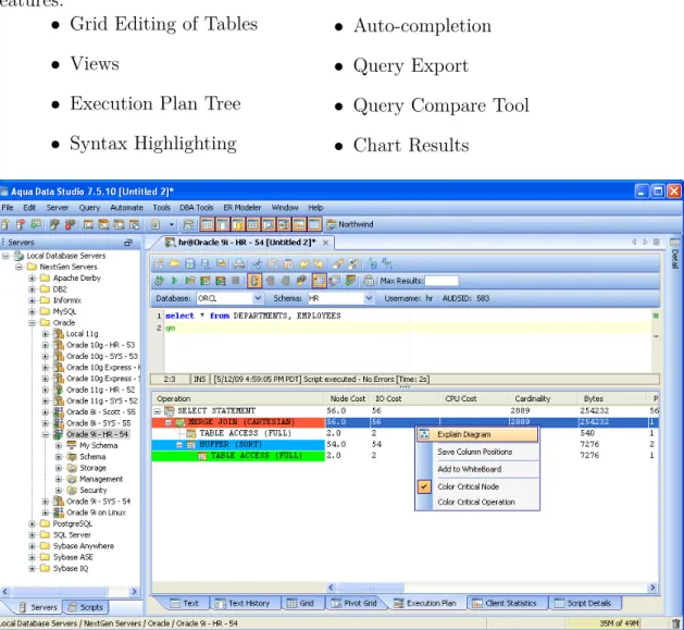
Aqua Data Studio

A commercial Query Analyser [9] which has many useful features like most com-mercial tools. Unlike the previous two tools it doesn’t support relational algebra but it has features that relational algebra tools lack. These are a few of the useful features:

• Grid Editing of Tables

• Views

• Execution Plan Tree

• Syntax Highlighting

• Auto-completion

• Query Export

• Query Compare Tool

• Chart Results

Figure 2.5: Aqua Data Studio Interface

2.6.6

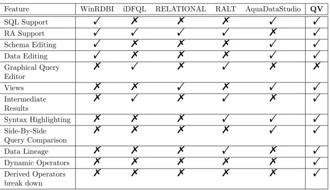
Features Comparison

Based on the characteristics of the described query analysers their features are out-lined in Table 2.3 along with what our implementation inherits from them. Graphical query editors, such as the one that iDFQL and RALT, clearly indicate the

interme-diate results of the evaluation. This is an important feature for a learning tool which the other non graphical editors do not provide. From another perspective we notice that the graphical editors are much harder to navigate and constructing complex queries is not practical mainly because they do not feet in one screen. Also there are some consistency issues when the user is trying to make changes. For example when deleting an operator, most of the times the whole query has to be reconstructed from the beginning.

Our attempt is to fill the gap between the two types of analysers by maintaining the same transparency to the evaluation process as the graphical editors but instead of graphical queries we will use textural queries which will help in constructing complex expressions. The user has the option to visualise the evaluation process in a tree structure composed with the operation nodes where each one provides a view of the result of the operation and cost information in terms of memory and time usage. Although the systems that support relational algebra make use of derived operators none of them shows to the user how the derived operator such asnatural joinis constructed using the basic operators. As a result there is no clear indication of the difference between the two. In our implementation all the derived operators can be specified by the user using an equivalent relational algebra expression with only basic operators. This will allow the user to introduce new operators and at the same time it will provide the option to convert a derived operator into a tree of basic operators when navigating the evaluation result.

Feature WinRDBI iDFQL RELATIONAL RALT AquaDataStudio QV

SQL Support ! % % % ! ! RA Support ! ! ! ! % ! Schema Editing ! % % % ! ! Data Editing ! % % % ! ! Graphical Query Editor % ! % ! % % Views % % ! % ! ! Intermediate Results % ! % ! % ! Syntax Highlighting % % % ! ! ! Side-By-Side Query Comparison % % % % ! ! Data Lineage % % % ! % ! Dynamic Operators % % % % % ! Derived Operators break down % % % % % !

Chapter 3

System Architecture

Before going into specific modules of the system we provide an overall system archi-tecture which describes what are the main tasks of the system and how they interact. The dependencies of each module are show in Figure 3.1. We follow the Model View Control (MVC) pattern with the aim to make future changes easier. The syntactical characteristics of a language should be independent from the semantics therefore we split the process into parsing and evaluation which have no dependency with each other.

3.1

View Layer

This layer is the graphical interface that the user interacts with. It consists of a query editor, a database browser and a results panel. For extensibility purposes no other module should rely on this. This will make future interface improvements much easier since the back-end of the system will not require any changes if we only need to fix graphical bugs or improve interface aesthetics.

3.2

Controlling Layer

All requests from the user will be handled by the respective controlling modules in this layer.

Query Controller

The query controller is responsible for handling query evaluation requests. It should call the respective modules in the lower layers in order to produce results. First it will call theParsing module that will generate a query tree and then it will request an evaluation of the tree against the data model from theEvaluation module.

Dependency System Architecture M o d e l C o n tr o lli n g V ie w QueryController QueryController.RA QueryController.ERA QueryController.SQL Visualiser(GUI) Persister DataModelController Module Layer DBImporter Parsing Parsing.RA Parsing.ERA Parsing.SQL Evaluation RelationalModel QueryTree Data Structure Figure 3.1: QV Architecture

Data Model Controller

The Data Model Controller is responsible for making changes to the data model as requested by the user in the View layer. Requests include database schema, data and stored queries (views) changes.

Persister

This module is responsible for storing the state of the workspace on stable storage. This should include the active data model and queries. It should support reloading of the workspace in the exact state that it was before the last save request.

3.3

Model Layer

Parsing

The module is responsible for parsing queries composed in RA, ERA or SQL. It should produce a query tree as a result.

Evaluation

The Evaluation module is responsible for evaluating a query tree on a data model. It assumes that the parsing phase has been successfully completed.

Relational Data Model

The Relational Data Model described here holds the data that the system will use to evaluate queries. The Data Model consist of a set of Relations and each relation holds a set of Attributes(Header) and a set of Rows(body) that satisfies the attribute conditions of the header. See 2.1 for more details.

Query Tree

Represents the structure used to host queries after parsing. It should have appro-priate structure to host the intermediate result and data lineage information of each node that theEvaluation Module will create when traversing the tree.

DB Importer

This module makes a connection to a database server and using queries on the server reconstructs a copy of the database using thesRelational Model structure.

Chapter 4

Query Representation and

Execution

At the core of the system is the query execution process which take as input a textural query (composed in RA, ERA or SQL) and populate a result by evaluating the query against the active data model. The process is split into parsing and evaluation. In this chapter we provide a complete design for both phases along with specification for a simple optimisation technique on query trees.

4.1

Query Syntax

In this section we cover the query syntax for RA, ERA and SQL which the parser implements. We will specify a suitable syntax for the RA and a minimalistic syntax for the SQL Select clause usingExtended Backus-Naur Form (EBNF) 1_.

4.1.1

RA Syntax

The basic syntax elements are described here plus an additional entry for the dynamic operators which can only be binary. The dynamic operators are derived operators that the user can define.

hinner operationi ::= <relation> | hunary operationi | hbinary operationi;

hoperationi ::= ‘(’ <inner operation>‘)’;

hunary operationi ::= hprojecti | hselecti | hrenamei;

hbinary operationi ::= hproducti | hunioni | hdifferencei |hdynamic operationi;

hrelationi ::= (letter)+;

hprojecti ::= ‘PROJECT’ ‘[’hattribute listi‘]’ hoperationi;

hselecti ::= ‘SELECT’ ‘[’ hboolean conditioni ‘]’ hoperationi;

hrenamei ::= ‘RENAME’ ‘[’ (letter)+ ‘/’ hattributei‘]’ hoperationi;

hproducti ::= hoperationi ‘PRODUCT’ hoperationi;

hunioni ::= hoperationi ‘UNION’ hoperationi;

hdifferencei ::= hoperationi ‘DIFFERENCE’ hoperationi;

hdynamic operationi ::= hoperationi (letter)+ (hboolean conditioni)?

hoperationi;

hattribute listi ::= hattributei ( ‘,’ hattributei)*;

hattributei ::= (letter)+ (‘.’ (letter)+ )?;

hboolean conditioni ::= (hboolean conditioni ‘OR’)? hand conditioni;

hand conditioni ::= (hboolean conditioni ‘AND’)? (‘NOT’)? hsingle conditioni;

hsingle conditioni ::= hboolean conditioni | hcomparisoni | hattributei;

hcomparisoni ::= hattributei | hstringi | hsigned integeri | hfloati;

hstringi::= “’ (alphanumeric)+ ‘”;

hsigned integeri ::= [‘+’ | ‘-’ ] hintegeri;

hintegeri ::= (digit)+;

hfloati ::= hsigned integeri‘.’ hintegeri;

4.1.2

ERA Syntax

The ERA syntax contains all the elements of the RA syntax with the following modifications/additions.

hunary operationi ::= hprojecti | hselecti | hrenamei | hgroupi | hdistincti | haggregatei;

hprojecti ::= ‘PROJECT’ ‘[’hattribute expression listi ‘]’hoperationi;

hrenamei ::= ‘DISTINCT’ hoperationi;

hgroupi ::= ‘GROUPBY’ ‘[hgrouping attributesi]’ hoperationi;

hattribute expression listi::= hattribute expressioni ( ‘,’ hattribute expressioni)*;

hattribute expressioni ::= hattributei | hattribute arithmetic expressioni hattribute arithmetic expressioni::= ((hfloati | hsigned integeri)

(‘+’|‘-’|‘*’|‘/’))* hattributei((hfloati | hsigned integeri) (‘+’|‘-’|‘*’|‘/’))*

haggregatei ::= haggregate functioni hoperationi;

hgrouping attributesi ::= (hattributei | haggregate functioni) ( ‘,’ (hattributei | haggregate functioni) )*;

4.1.3

SQL Syntax

hselect expressioni ::= ‘SELECT’ [‘DISTINCT’ | ‘ALL’ ] hcolumn expri* ‘FROM’ hfrom expri [ ‘WHERE’ hwhere expri ] [’GROUP BY’hattribute listi* ] [ ‘HAVING’ hconditioni ] [‘ORDER BY’horderby expri ]

hcolumn expri::= hidenti [ ’AS’ ] [hidenti ]

hfrom expri::= htablei[ ’,’ hfrom expri ]

hfrom expri::= htablei[INNER | [[LEFT|RIGHT|FULL] [ OUTER ]] |

NATURAL ] JOINhtablei [ON <condition>]

horderby expri ::= hidenti [ ’ASC’ | ’DESC’] [’,’hidenti [ ’ASC’| ’DESC’]]*

4.1.4

Syntax Errors

The parser will identify syntactical errors and report them. Where applicable it will provide position information for the error in the query.

4.2

Query Tree

When the input is validated and there are no syntax errors the parser will construct a Query Tree that will be used in the evaluation process. The result tree contain only three types of nodes: unary operators , binary operators and relations (leaf) nodes.

For example the the following RA query translates to the tree in Figure 4.2: P ROJ ECT[R.A, S.A, S.B](R P RODU CT(SELECT[S.B > S.C]S))

Unary Operation Parameters:[ a1, .., an] Child Operation R Binary Operation Parameters:[ a1, .., an] Child Operation Left } } zzzzzz zzzzzz zzzzz Child Operation Right ! ! C C C C C C C C C C C C C C C C C C R S

Figure 4.1: Unary and Binary Abstract Operation Trees

When translating a RA or ERA query to a tree we will use operations (nodes) that arise in the syntax of the respective language. In the case of SQL we will translate it to an ERA tree that is similar to the low-level operations that most RDBMS use. By doing so we can later display this ERA tree to the user in order to provide an insight on how SQL is translated and executed. At the parsing stage

Project(π)

Parameters:[ R.A, S.A, S.B]

Cartesian Product(×) Parameters:null x x pppppp pppppp pppp ) ) S S S S S S S S S S S S S S R Select(σ) Parameters:[S.B>S.C] S Figure 4.2: Operation Tree Example

we don’t check if the query is referencing valid attributes or relations since the evaluation engine will be responsible for identifying this at the next stage.

4.3

Query Evaluation

The evaluation engine consist of specialist evaluators and a general evaluation mod-ule (entry point) which take as input a Query Tree and a Relational Data Model and evaluates the tree on the model in order to return a result (table).

4.3.1

General Evaluation Module

Determines the type of the tree head node (e.g. Project operator) and calls the relevant specialist module to evaluate it.

4.3.2

Specialist Evaluation Modules

Each of the following specialist modules will evaluate a query tree of the respective type.

Relation Evaluator: Using the data model it retrieves and returns the table with the specified name from the database.

Project Evaluator: Requests evaluation for child sub-tree by calling the general evaluator. From the result it removes attributes that are not included the list of

SpecialistM odules Product Evaluator Project Evaluator QueryTree DataModel ) ) S S S S S S S S S S S S S S S S S S S S S S S S S S Select Evaluator General Evaluator table(output) u u kkkkkkkk kkkkkkkk kkkkkkkk kk z z : : u u u u u u u u u u u u u u u u u u u u u u u u u u u u u u u uu 5 5 j j j j j j j j j j j j j j j j j j j j j j j o o // i i ) ) T T T T T T T T T T T T T T T T T T T T T T T d d $ $ I I I I I I I I I I I I I I I I I I I I I I I I I I I I I I I ^ ^ > > > > > > > > > > > > > > > > > > > > > > > > > > > > > > > > > > > > > > > > > [ [ 6 6 6 6 6 6 6 6 6 6 6 6 6 6 6 6 6 6 6 6 6 6 6 6 6 6 6 6 6 6 6 6 6 6 6 6 6 6 6 6 6 6 6 6 6 6 6 6 6 6 @ @ Relation Evaluator Rename Evaluator Union Evaluator Difference Evaluator Dynamic Evaluator Figure 4.3: Evaluators Collaboration Diagram

attributes (parameter).

Select Evaluator: Requests evaluation for child sub-tree. From the result it re-moves rows that do not satisfy the selection condition(parameter).

Rename Evaluator: Requests evaluation for child sub-tree and renames the at-tribute specified in the parameter with the new name.

Cartesian Product Evaluator: Requests evaluation for child sub-trees and cre-ates a new table with all attributes from both results. It then adds rows by combining all possible pairs from the two results(i.e. R×S).

Union Evaluator: Requests evaluation for child sub-trees. Checks that their at-tributes are compatible and returns a new table by including all rows from both sub-trees.

Difference Evaluator: Request evaluation for child sub-trees. Checks that their attributes are compatible and returns a new table by including all rows from the left sub-tree and deleting any rows that occur in the second sub-tree too.

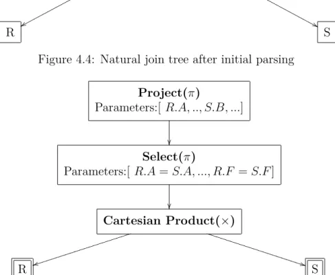
Dynamic Evaluator: It finds the definition of the operator in a repository. It parses the definition which results in a new tree which it then requests a new com-plete evaluation for. In other words it will convert a derived operation into a tree of operations as specified by the definition of the derived operator. We illustrate this with the case of Natural Join:

PROJECT[#REF1 UNION #REF2] ( SELECT[#REF1.$=#REF2.$] (

#REF1 PRODUCT #REF2 )

);

This definition states that the result is the projection of all unique attributes of the two relations (#REF1 UNION #REF2) and the body of the result contains all rows that agree on all common attributes (#REF1.$=#REF2.$). Assume this definition is stored in the set of derived operators under the name ‘NATURALJOIN’ and the query "S NATURAL JOIN R" is being evaluated. The parser will initially parse this and create the tree in Figure 4.4. When the evaluation begins the Dy-namic Evaluator will transform this into the tree in Figure 4.5 where the selection will match all common attributes and the projection includes all unique attributes of both R and S.

4.3.3

Evaluation Errors

Evaluation errors arise when the query tree cannot be evaluated against the data model because of missing relations or attributes. The Project, Select and Rename evaluators should check for missing attributes and report them. the missing relation

Derived Operation

Parameters:[ op_name="NATURALJOIN"]

x x pppppp pppppp pppppp pppppp p & & N N N N N N N N N N N N N N N N N N N N N N N N N R S

Figure 4.4: Natural join tree after initial parsing

Project(π)

Parameters:[ R.A, .., S.B, ...]

Select(π)

Parameters:[ R.A=S.A, ..., R.F =S.F]

Cartesian Product(×) t t iiiiiiiiii iiiiiiiiii i * * U U U U U U U U U U U U U U U U U U U U U R S

Figure 4.5: Natural join tree after expansion to original definition

case will only need to be tracked in the Relation Evaluator. In addition the Union and Difference evaluators should check attribute compatibility of the two sub-tree results (i.e. check that both sub-trees contain the same attributes). These errors are used by the user interface that gives visual feedback to the user.

4.3.4

Views

Queries composed by the user can be stored in the Relational Data Model as Views. Each view is assigned a name and it can be referenced in a different query as any other base relation of the Data Model. To make the system as generic as possible both SQL and RA views can be stored and queries can reference views of different type, for example we can reference an SQL view in a RA query. The evaluation engine will retrieve the query of the referenced view and execute it. After that it will treat it as a base relation.

4.3.5

Execution Statistics

We can derive execution time and memory usage statistics by capturing the time spent evaluating each node and the average row size along with the number of rows of the result. We demonstrate this with an example. Evaluation of the query tree in Figure 4.2 will update the tree so that it includes time and memory measures for each node as in Figure 4.6. The statistics and data lineage (Section 4.3.6) are not data that would occur in a normal execution therefore are not considered in the statistical calculations.

Project(π)

Parameters:[ R.A, S.A, S.B] ExecutionTime= 30ms RowSize=15kB RowCount=3750 Cartesian Product(×) Parameters:null ExecutionTime= 25ms RowSize=50kB RowCount=3750 z z tttttt tttttt % % J J J J J J J J J J R ExecutionTime= 5ms RowSize=25kB RowCount=75 Select(σ) Parameters:[S.B>S.C] ExecutionTime= 15ms RowSize=25kB RowCount=50 S ExecutionTime= 5ms RowSize=25kB RowCount=100 Figure 4.6: Operation Tree Example with statistics

Execution Time

From the time span logged at every node we can derive the following:

• Overall Execution Time: Execution Time of Head node.

• Sub Tree Execution Time: Execution Time of Head node of sub-tree.

• Operation Contribution Time: Execution Time of operation node minus Exe-cution Time of children.

In the case of our example we can deduce the contribution of each operation performed:

• Load relation S Contribution Time = 5ms= 5ms−(0ms)

• Load relation R Contribution Time = 5ms= 5ms−(0ms)

• Select Contribution Time = 10ms= 15ms−(5ms)

• Cartesian Product Contribution Time = 5ms= 25ms−(5ms+ 15ms)

• Project Operation Contribution Time = 5ms= 30ms−(25ms)

• Overall Execution Time= 30ms Memory Usage

The size of each intermediate result calculated by an operation is estimated by mul-tiplying the number of rows with the average row size. From this we can further derive maximum memory usage during evaluation of a tree. During an operation we evaluate the child operations and keep their results until the end of the evaluation. Assuming that sub-trees can be processed in parallel we can define the maximum memory usage using Equation 4.1. This is the worst case scenario because if oper-ations are executed sequentially, then the memory usage is less.

maxmemory(x) = max " resultsize(x) + nx X i=0 resultsize(ix) ! , nx X i=0 maxmemory(ix) # (4.1) where nx is the number of children of node x and ix represents the i-th child node

of x.

• MaxMemoryUsage(Load Relation S)= 2500kB = max [(25∗100) + (0),0]

• MaxMemoryUsage(Load Relation R)= 1875kB = max [(25∗75) + (0),0] • MaxMemoryUsage(Selection)= 3750kB = max [3750,1875] = max [(50∗25) + (2500),1875] • MaxMemoryUsage(Cartesian Product)= 190625kB = max [190625,5625] = max [(50∗3750) + (1875 + 1250),1875 + 3750] • MaxMemoryUsage(Projection)= 243750kB = max [243750,190625] = max [(15∗3750) + (187500),190625]

4.3.6

Data Lineage

To allow the user to drill down and see from where specific rows of the result comes from we need to add some overhead to our query tree during the evaluation process. In particular we create one map for every arc in the tree which is stored on the parent node. This map will contain entries linking rows of the parent node to rows in the child node. The maps should be created based on the following rules for each operator:

Unary Operations

Each row of the operation result should map to the row of the child that it derived from.

• Project and Rename One to One relation. The number of entries should equal the number of rows.

• Select One to One relation. The number of entries should equal the number of rows that satisfy the selection condition.

• Group One to Many relation. Each row of the result maps to all rows of the child that agree on the group by attributes.

Binary Operations

Each row of the operation result should map to the rows of the children that it derived from(i.e. two maps, one per child (arc))

• Cartesian Product Many to Many relation. Each row has an entry in both maps with the rows that it combines.

• Union One to Many relation. Each row of the result maps to one row of a child or one row of each child.

• Difference One to One relation. Each row of the result maps to one row of the first child. An additional map is created indicating rows that have not been included because they were part of both the left and right child(implicit contribution to result).

We don’t need to specify rules for derived operators since they are always evalu-ated using the basic operators and the lineage rules are therefore always inherited.

4.4

Algebra Optimisation

We will specify a systematic way of improving execution performance by simple tree modifications which do not affect the end result of the query. We focus on moving selections to the lowest possible level of the query tree in order for them to be evaluated early and limit the size of the intermediate result that parent nodes need to work on. There are two general cases that arise. The first one is when the input operation (child node) of the selection is a unary operation and when it is a binary one. Implementing the following simple rules will yield an efficient selection strategy. Here we need to acknowledge the fact that some of these optimisations will not always improve the memory usage and a more sophisticated approach using database statistics can be employed to tackle this issue. Such an approach is out of the scope of the project although we design a platform that is capable of hosting such extensions.

4.4.1

Unary Input Case

In general if all the referenced attributes in the selection condition are part of the heading2 of the child’s input then it is safe to switch the select operation with its child. To avoid the computation of result headings and improve performance during optimization we can take a simpler approach. If the child operation isproject then we move the selection as the child. If the operation is rename and the renamed attribute is not referenced in the select condition we move the selection as the child. If the child operation is another selection we combine the two operations into one using the booleanand connective. This will eliminate the redundant iterations.

4.4.2

Binary Input Case

We split the select condition based on the booleanand operators and we derive a set of sub-expression. We then decide for each such expression whether all its referenced attributes are part of the heading of only one of the children of the immediate binary operator. If so, we add a selection operation above that child. The sub-expressions that could not be matched to only one child are joined again with the boolean and

Chapter 5

Workspace and Visualisers

In this chapter we define the graphical interface of the system. We go through the various features of the QV workspace shown in Figure 5.1. The implementation details of the system are described in Chapter 6.

5.1

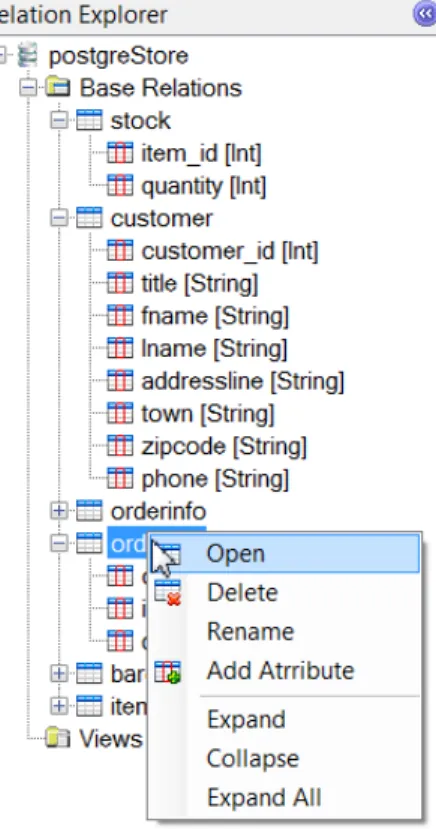
Relation Explorer

Figure 5.2: Relation Explorer In order for the user to execute queries a database

should be constructed first. There is no support for a Data Definition Language but schema and data editing can be achieved from the graphical inter-face. For this purpose like most query analysers the schema of the active database in the application is shown in a tree structure in the relation explorer on the left of the workspace. It is split into two sub-trees, Base Relations and Views. In Base Rela-tionsall the relations are listed with their attributes and their respective data types. The user can make changes to the database schema by adding delet-ing and editdelet-ing relations and attributes. These op-tions are available in the right click context menu and on the main tool bar. In order to modify the rows of a relation the user can either use the context menu "Open" option or double click on the relation name and a new window with a tabular grid will be created on which the user can make the relevant changes. When adding new relations or editing the name of an attribute we use a defensive approach to the name clashes problem by disabling the relevant options. For example if the user defines a new rela-tion with the name "item" which already belongs to the database the modal "New Relation" dialog box will warn the user(Figure 5.3). Same approach has

been followed for many cases such as creating a new view and editing the definition of an attribute (name and data type). The relation explorer panel can be collapsed using the button on the top right corner or from theView menu on the menu bar.

5.2

Import

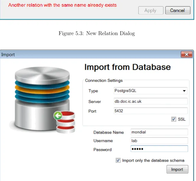
The system allows data import from an existing database. Given a connection string it can replicate the schema and the data (excluding views and procedures). This should be stored into an instance of a Data Model that the system will be able to use in query evaluation. After the import is completed the user can use schema and data editing to make further database changes. These changes will not reflect the actual database used but they will only update the local data model.

Figure 5.3: New Relation Dialog

Figure 5.4: Import from database dialog

5.3

Tab Containers

To make the environment generic and customisable based on the user preferences the main area of the workspace can host multiple tab windows which can be query editors or relation grid editors. Also the user has the option to open a second tab

container to gain visual access to two windows at the same time. This is useful in cases that we want to see the difference between two queries illustrated in Figure 5.5.

Figure 5.5: Two tab containers

5.4

Query Panel

The main component of the interface is thequery panel which is split into two areas. The top one consists of an editor where the user specifies a query and the bottom one which displays the query results (Figure 5.6). We describe each one in detail in Sections 5.5 and 5.6 respectively. When the user creates a newquery panel from the menu there are three options which open the panel in relational algebra, extended relational algebra or SQL mode.

5.5

Query Editor

The query editor provides appropriate highlighting to help the user spot mistakes easily. Highlighting is split into two types.

Figure 5.6: Query Panel

• Matching Brackets Indicator

When the editor caret is at bracket and there is a matching opening or closing one they are both highlighted. This is a standardised way that many inte-grated development environments (IDEs) use and we can expect the user to be familiar with this method.

• Syntax Recognition

In a similar way we inherit the syntax highlighting principles. The syntax keywords are recognised and highlighted accordingly. When editing a query, basic operators are highlighted with blue and the derived operators in purple.

In addition relation and attribute names of the active database are also dynam-ically recognised and highlighted in green. Constant values are also indicated,

strings and numeric values are highlighted in red and blue respectively.

Derived Operator Editor

Using the syntax we specified for defining derived operators in Section 4.1 we also incorporated another editor with the same highlighting mechanism as the query editor that allows the user to define new and edit existing operators. When adding such an operator the user specifies the name of the operator, it’s definition and an icon to represent the operator in the results tree.

Figure 5.7: Derived Operator Editor

5.6

Result Visualisers

The result of a query evaluation are presented in the results panel below the query editor. There are five available options and each one serves a different purpose:

5.6.1

Data Grid

This is the simplest view which is an integral part of every query analyser. It displays the result of the query execution in a read only tabular grid. As an additional feature the rows of the grid can be sorted by clicking on the column headers.

5.6.2

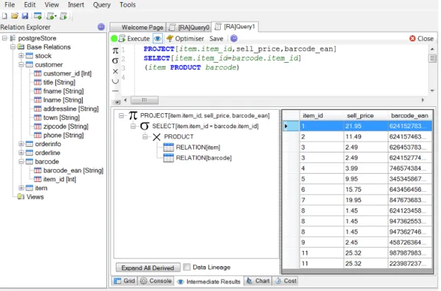
Intermediate Results

As we explained earlier we need to emphasise on how we display query results to the user. This view provides an analytical description of the evaluation process using a tree structure that represents the query tree as described in Section 4.2. This tree is used as a navigation mechanism. When the user clicks on a node the intermediate result calculated at that node during evaluation is displayed on a grid on the right.

Figure 5.8: Intermediate Results View

Derived Operators Break Down

The derived operator nodes are highlighted with light blue. In the case that such an operator occurs in the tree the user can select to expand it which will transform the operator into a tree of operations based on it’s definition as illustrated in Figure 5.9.

−→

Data Lineage

To provide a more detailed explanation on how the result was obtained the user can select rows in the grid of the head node and automatically all the rows directly associated in all child nodes will be highlighted. Information on how to find these rows can be derived from the mappings created during query execution in Section 4.3.6. In addition when a grouping operator is used the user has the option to open a new window that will display on a grid the different groups of rows that formed the result.

Figure 5.10: Selecting Rows for Lineage

5.6.3

Chart

Whenever execution contains numeric values the chart view can draw interactive charts for a selection of numeric attributes grouped by a specified attribute. The chart has many options such as zooming and stretching along both axes and it can also be exported into an image in various formats. An example of a query displayed using a chart is shown in Figure 5.12.

5.6.4

Console

A simple but essential view that will indicate whether the execution was successful or if any errors occurred. If it was successful then the execution time and the number of rows are printed. In the case that there was an error it indicates if the error was a syntax or evaluation error along with information on the source of the error when applicable. Both type of messages are timestamped and represent the log of the evaluation engine actions.

Figure 5.13: Console

5.6.5

Execution Cost

In Section 4.3.5 we explained how we can calculate various statistical measures of the execution. The user has the option to browse through these statistics. The Cost view will also be accompanied with a query tree like the intermediate results which will serve as a navigation mechanism in order to find statistics specific to each operation performed. The percentages of the evaluation time needed to evaluate the selected operator and the whole (sub) tree are shown using progress bars. The

Initial Cost group indicates the time spent evaluating the child nodes therefore the execution time is less than the total time. Also there is a summary of the size of the output table at the node which shows the number of rows, the average row size and the overall size in bytes.

Figure 5.14: Execution Cost View

5.7

Visual Optimiser

The user can request from QV to optimise a query using the "Optimise" button on the tool bar above the query editor. This will create a new tab window with the tree structure of the query. In this window the system will apply the optimisation rules described in Section 4.4. The user can browse a series of trees that transform step by step the original tree to the most optimised one. In the tree browser the user can see the current state and the previous state as shown in Figure 5.15. Each time the browser proceeds to the next step the nodes that have been added or changed are highlighted with green. Also the previous state tree highlights in red the nodes that have changed.

There is an option to execute all the trees generated or only the most optimised. If all of the trees are executed a detailed statistics view is displayed which shows similar information as the Execution Cost View (5.6.5) with additional charts and graphs that compare the performance of each tree at the different stages of the optimisation.

5.7.1

Tree Execution Time

A bar chart that compares the execution time of each optimisation state with nanosecond accuracy. The optimiser in Figure 5.15 shows this view on the bot-tom section.

5.7.2

Tree Maximum Memory Usage

A bar chart that compares the maximum memory usage based on Equation 4.1. The memory size is calculated in bytes and an example is shown in Figure 5.16.

Figure 5.16: Maximum memory usage per tree

5.7.3

Operation Nodes Execution Time

For every state of the optimisation process the user has the option to view a pie chart that shows what percentage of the execution time each operation consumed. The pie chart included a legend that helps identifying the operations using the pie chart colours. In addition when the mouse cursor is on a specific piece of the chart the tool tip will indicate the operation as well. This is useful in cases that there are many operators and colours can not be distinguished. An example is shown in Figure 5.17.

Figure 5.17: Execution time per operation

5.7.4

Operation Memory Usage

This is the last statistical view which shows for every state of the optimisation the memory usage of each operation performed. Also in a different colour (blue) the output size of the operation is shown. The purpose for displaying the two together is to see how close the two lines are to each other compared to other evaluations. This provides information on how quickly the evaluation drops redundant data.

Chapter 6

Implementation Details

We developed QV based on the designed described in the previous chapters. Here we describe the most important details of the implementation. The main focus is on the parsing and evaluation process and how they produce the results as presented in the graphical interface described in Chapter 5. We emphasis on the modularity of the system and show how future changes can be incorporated.

6.1

Overview

The implementation is split into several packages that can be compiled and be distributed independently as dynamic-link libraries (DLLs). Each such package serves a different purpose and are all based on the architecture described in Chapter 3. The packages that form QV are shown in Figure 6.1 with arrows showing the calls that each package makes to another. In addition to the dependencies implied by the arrows, packages are also dependent with lower layers (i.e. lower in the diagram) but there are no upward or cyclic dependencies.

6.2

Graphical Interface

All the graphical interface components, including classes and images are contained in the QV.Visualiser package. The main entry point is the Visualiser class which contains the various panels that form the application workspace. The rest of the classes are distributed in the following sub-packages:

• QV.Visualiser.RelationExplorer: Contains classes that form the database browser on the left side of the workspace.

• QV.Visualiser.Viewer: The main tab container along with the relevant tab controls such as query, grid or optimiser tabs that can be drawn in the tab container. The important components of this package are the various classes that display the result of the query execution. For example, the StatisticsRe-sultsControl class is responsible for