On moments and related quantities in insurance surplus analysis

(1)

On Moments and Related Quantities

in Insurance Surplus Analysis

by

Wing Yan Lee

A thesis

presented to the University of Waterloo in fulfillment of the

thesis requirement for the degree of Doctor of Philosophy

in

Actuarial Science

Waterloo, Ontario, Canada, 2014 c

(2)

Author’s Declaration

I hereby declare that I am the sole author of this thesis. This is a true copy of the thesis, including any required final revisions, as accepted by my examiners.

(3)

Abstract

In risk theory, the time to ruin is one of the central quantities. The Laplace transform, density and moments of the time to ruin have been studied by many authors under different risk model assumptions. The Gerber-Shiu function proposed by Gerber and Shiu (1998) provides an analytic tool in studying these quantities. For example, Dickson and Willmot (2005) inverted the Gerber-Shiu function with respect to the Laplace transform parameter of the time to ruin by Lagrange’s implicit function theorem, and hence obtained the density of the time to ruin. The main focus of this thesis is to study the moments involving the time to ruin by using Gerber-Shiu function as the analytic tool. An introduction on the Gerber-Shiu function and different risk models is first given in Chapter 1.

In Chapter 2, the moments of the time to ruin are studied as generalized versions of the Gerber-Shiu function in dependent Sparre Andersen models. It is shown that structural properties of the Gerber-Shiu function hold also for the moments of the time to ruin. In particular, the moments continue to satisfy defective renewal equations. These properties are discussed in detail in Chapter 4 under the model of Willmot and Woo (2012) where Coxian interclaim times and arbitrary time-dependent claim sizes are assumed. In Chapter 3, another very general class of dependent Sparre Andersen models with Coxian claim sizes (e.g. Landriault et al. (2014)) is considered. An analytical form is provided for the moments of the time to ruin under this class, which involves solving linear systems of equations.

In Chapter 5, the number of claims until ruin is taken into consideration under a Sparre Andersen model with exponential claim sizes. The joint density of the time to ruin, the number of claims until ruin and other ruin-related quantities is identified. The joint moments of these quantities can then be obtained from this joint density.

(4)

model introduced in Cheung et al. (2011). With Coxian claim sizes, the moments of the time to ruin are in the form of a linear sum of Erlang densities. The associated coefficients of this linear sum are shown to satisfy linear systems of equations.

Finally, a brief conclusion of this thesis and a discussion of future research are given in Chapter 7.

(5)

Acknowledgements

I would like to thank my supervisor, Professor Gordon E. Willmot for all his support and guidance in writing this thesis. Thanks are also given to Professor Steve Drekic, Professor David Landriault, Professor Qi-Ming He and Professor Qihe Tang for their useful suggestions on this thesis.

(6)

Dedication

(7)

List of Tables

1.1 Value of ruin-related quantities when NT = 1 and NT >1 . . . 5

3.1 Joint pdf of interclaim times and claim sizes: independent cases . . . 41 3.2 Joint pdf of interclaim times and claim sizes: dependent cases . . . 43

5.1 Approximate and exact values of E[T I(T < ∞)|U0 =u] by (5.53) and (5.58) 92

(11)

List of Figures

3.1 Comparison of the expected time to ruin in independent cases . . . 41

3.2 Comparison of the variance of time to ruin in independent cases . . . 42

3.3 Comparison of the expected time to ruin in dependent cases . . . 44

3.4 Comparison of the variance of time to ruin in dependent cases . . . 45

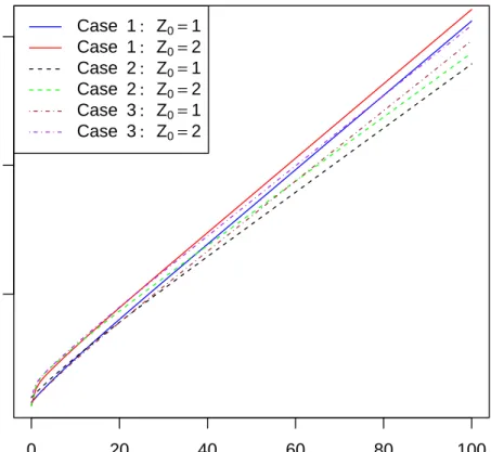
4.1 Approximate and exact values of E[T|T < ∞, U0 =u] . . . 67

4.2 Approximation of E[T|T < ∞, U0 =u] . . . 68

6.1 Probability of ruin in different cases . . . 114

(12)

Chapter 1

Introduction and background

In this chapter, the insurance surplus process is first introduced. Details are given on the dependent Sparre Andersen model and the MAP risk model. The Gerber-Shiu function and the moments of ruin-related quantities are then discussed. Mathematical preliminaries that are useful in this thesis are given at the end.

1.1

Dependent Sparre Andersen risk model

The insurance surplus process {Ut, t≥0} is usually modelled by

Ut=u+ct− Nt

X

i=1

Yi, (1.1)

where u (u ≥ 0) is the initial surplus and c is the premium rate in one unit of time.

{Nt, t≥0}is a claim number process which is defined through a sequence of independent

and identically distributed (iid) interclaim time random variables{Vi, i= 1,2, . . .}, where

(13)

i= 2,3, . . .. {Yi, i= 1,2, . . .}is a sequence of claim size random variables which is iid. The

pairs {(Vi, Yi), i= 1,2, . . .}are iid, but Vi and Yi may be dependent. (1.1) is known as the

dependent Sparre Andersen model (and simply known as the Sparre Andersen model if Vi

and Yi are independent for all i = 1,2, . . .). See for example Sparre Andersen (1957) and

Rolski et al. (1999) for references on this model.

Let the marginal probability density function (pdf) and cumulative distribution func-tion (cdf) of the interclaim timeV bek(t) and K(t) respectively, whereV is any arbitrary Vi. On the other hand, the marginal pdf and cdf of the claim size Y are denoted by p(y)

and P(y) respectively, where Y is any arbitrary Yi. Also, let f(t, y) be the joint pdf of

the pair (V, Y) when V = t and Y = y. Finally, let us assume that the positive security loading condition

E[cV]> E[Y] (1.2) holds in (1.1).

The classical Poisson risk model is one of the well-known special cases of the dependent Sparre Andersen model. In this model, the joint pdf of the interclaim time and claim size is given by

f(t, y) = λe−λtp(y).

In other words, the classical Poisson risk model assumes that {Vi, i = 1,2, . . .} are

inde-pendent of {Yi, i= 1,2, . . .}and {Vi, i= 1,2, . . .}follow exponential distribution. Readers

may refer to e.g. Gerber (1979), Grandell (1991) and Panjer and Willmot (1992) for a complete introduction on the classical Poisson risk model. There are also studies on the dependent Sparre Andersen model with more general interclaim times and claim sizes. Recent examples include Albrecher and Teugels (2006), Boudreault et al. (2006), Cossette et al. (2008), Zhang et al. (2012) and references therein.

(14)

1.2

Ruin-related quantities and Gerber-Shiu function

1.2.1

Gerber-Shiu function

LetT be the time to ruin for the process{Ut, t≥0}, which is defined by

T = inf{t≥0 :Ut<0} (1.3)

and T = ∞ if Ut is non-negative for all t ≥ 0. The Gerber-Shiu function introduced in

Gerber and Shiu (1998) is defined as

mδ(u) = E[e−δTw(UT−,|UT|)I(T <∞)|U0 =u], (1.4) whereδ ≥0, the penalty function w(x, y) satisfies mild integrablility conditions and I(A) is an indicator function which takes value 1 if the event A occurs and 0 otherwise. The random variables UT− and |UT| represent the surplus before ruin and the deficit at ruin

respectively. Before the Gerber-Shiu function was introduced, the joint density of UT−

and |UT| had been studied in Dufresne and Gerber (1988) under the classical Poisson risk

model. The probability of ruin

m0(u) =E[I(T < ∞)|U0 =u] is a special case of (1.4) withδ = 0 andw(x, y) = 1.

Under the classical Poisson risk model, it was shown in Gerber and Shiu (1998) that (1.4) follows a defective renewal equation. Lin and Willmot (1999) gave the solution to this equation in the form of a compound geometric tail. The Gerber-Shiu function is also considered in more general Sparre Andersen model. For example, Dickson and Hipp (2001), Li and Garrido (2004) and Gerber and Shiu (2005) studied with Erlang interclaim

(15)

time. Willmot (2007) and Landriault and Willmot (2008) further the studies with arbitrary interclaim time.

There is also literature on the Gerber-Shiu function in dependent Sparre Andersen model. Albrecher and Boxma (2004) assumed a Markovian claim arrival process. Badescu et al. (2009) considered a bivariate phase-type distribution for the interclaim time and the claim size. Albrecher et al. (2011) introduced dependence by mixing distribution.

Next, let us denote the number of claims until ruin byNT, which is also a widely studied

random variable in risk theory. Stanford et al. (2000) developed a recursive method through the number of claims until ruin in order to calculate the probability of ruin. Egidio dos Reis (2002) studied the distribution of the number of claims until ruin under the classical Poisson risk model. In Landriault et al. (2011), the number of claims until ruin is introduced to the Gerber-Shiu function as

mr,δ(u) =E[rNTe−δT−sUT−I(T <∞)|U0 =u], (1.5) wherer ∈(0,1] and s ≥0. With exponential claim sizes, closed form expression for (1.5) is obtained in the paper.

In Cheung et al. (2010), another generalization of the Gerber-Shiu function that also involvesNT is proposed as

mδ(u) =E[e−δTw(UT−,|UT|, XT, RNT−1)I(T <∞)|U0 =u] (1.6)

forδ ≥0. Xt denotes the minimum surplus before time t, i.e. Xt= inf

0≤s<tUs. Rn is defined

as R0 =u and Rn = u+P_in₌₁(cVi−Yi) for n = 1,2, . . .. Therefore, XT is the minimum

surplus before ruin. RNT−1 is equal tou if ruin occurs on first claim, and for ruin occurs

on claim subsequent to the first, it is the surplus immediately after the second last claim before ruin.

(16)

Ruin-related quantities NT = 1 NT >1 UT− UT− UT− |UT| |UT| |UT| T UT−−u c inf{t≥0 :Ut<0} XT u inf 0≤s<TUs RNT−1 u u+ PNT−1 i=1 (cVi−Yi) Table 1.1: Value of ruin-related quantities when NT = 1 andNT >1

1.2.2

Moments of ruin-related quantities

In Gerber-Shiu function (1.4), the (joint) moments of the surplus before ruin and the deficit at ruin is easily obtained by considering the penalty function

w(x, y) =xkyn,

where k and n are non-negative integers. Lin and Willmot (2000) showed that the mo-ments of the surplus before ruin and the deficit at ruin can be expressed analytically using compound geometric tails in the classical risk model.

Next, consider the moments of the time to ruin which may be studied in two approaches. The first approach is to determine the (defective) density of the time to ruin and obtain the moments of the time to ruin by integration. To be specific, suppose the (defective) density of the time to ruin given initial surplus u is g(t|u), then the kth moment of the time to ruin can be calculated as

E[TkI(T <∞)|U0 =u] = Z ∞

0

(17)

for k = 0,1,2, . . .. The density of the time to ruin has been studied with different model assumptions in the literature. Drekic and Willmot (2003) determined the density of the time to ruin under the classical Poisson risk model with exponential claim sizes. In a classical Poisson risk model with arbitrary claim sizes, Dickson and Willmot (2005) inverted the Gerber-Shiu function to determine the density of the time to ruin by Lagrange’s implicit function theorem (e.g. Good (1960) and Goulden and Jackson (1983)). This result was generalized in Landriault and Willmot (2009) where the joint distribution of the time to ruin, the surplus before ruin and the deficit at ruin was given. Recently, Landriault and Shi (2013) assumed combination ofn exponentials claim sizes and obtained the density of T by multivariate Lagrange expansion.

The second approach to study the moments of the time to ruin is by noting that they are closely related to the Gerber-Shiu function. To see this, let us consider

mδ(u) =E[e−δTI(T <∞)|U0 =u]

without loss of generality. (If joint moments of the time to ruin and other ruin quantities are of interest, then consider mδ(u) with an appropriate penalty function). Define the

discountedkth moment of the time to ruin as

mk,δ(u) = E[Tke−δTI(T <∞)|U0 =u], (1.7) where k = 0,1,2, . . ., then it is obvious that (1.7) can be obtained by differentiating the Gerber-Shiu functionkth times with respect to δ, i.e.

mk,δ(u) = (−1)k

∂k

∂δkmδ(u). (1.8)

To show that the above differentiation is valid, one can apply the Lebesgue’s dominated convergence theorem (e.g. Resnick (2005)). The Lebesgue’s dominated convergence theo-rem can be applied when the integrand of mδ(u) = E[e−δTI(T < ∞)|U0 = u] is assumed

(18)

to satisfy mild integrability conditions. These conditions implicitly follow from the tacit assumption that all moments of the time to ruin considered in this thesis are finite. For more general Gerber-Shiu functions, these integrability conditions impose restrictions on the penalty functions involved. For evaluation of marginal moments of the time to ruin, it may be assumed that the penalty function is 1.

Under the classical Poisson risk model, Lin and Willmot (2000) gave a recursive equa-tion for the moments of the time to ruin. The equaequa-tion was solved in Willmot (2002) by using the compound geometric distribution and its higher-order equilibrium distributions. These results were recursive in nature and hence involved complicated calculation. Hence, Drekic et al. (2004) and Drekic and Willmot (2005) studied these results from a com-putational point of view and provided numerical examples by assuming phase-type claim sizes.

There are also studies on the moments of the time to ruin under more general risk models. For example, Dickson and Hipp (2001) considered a Sparre Andersen model with Erlang(2) interclaim times, and Li and Lu (2013) assumed a surplus process with interest.

1.3

MAP risk model

There are also studies on the risk model with a Markovian arrival process (MAP). Interested readers may refer to Neuts (1979) and Latouche and Ramaswami (1999) for introduction on MAP. Many papers, e.g. Ahn and Badescu (2007) and Cheung and Landriault (2010), had analysis of the Gerber-Shiu function in a MAP risk model. In Yu et al. (2010), the moments of the time to ruin were studied in a MAP risk model with phase type claim sizes. A brief description of the MAP risk model, mainly based on Cheung et al. (2011), is given in the following.

(19)

For a MAP, it involves a homogeneous continuous-time Markov chain (CTMC). Let this CTMC beY ={Y(t), t ≥0}defined on a finite state spaceS ={1, . . . , m}. In the context of a risk model, CTMC Y may involve two kinds of transitions which are represented by the transition rate maticesD0 and D1 respectively. The (i, j)th entry of

1. D0, where i6=j, is the transition rate the CTMC Y changes from state ito state j with no claim happening;

2. D1 (i=j is also being considered), is the transition rate the CTMCY changes from state i to state j with a claim happening.

For convenience, either kind of transition will be referrred as a system change in this section and in Chapter 6. The (i, i)th entry of D0 is negative and its absolute value is equal to the rate of a system change given that the CTMCY is in statei. The sum of the ith row ofD0+D1 should add up to zero. For a MAP risk model, if the CTMC is in state i, the waiting time of a system change follows an exponential distribution with mean equals to the absolute value of the inverse of the (i, i)th entry of D0.

The MAP includes many well-known processes as special cases. Whenm = 1,D1 = (λ) and D0 = (−λ), the MAP reduces to a homogeneous Poisson process with arrival rate λ. When D1 =         λ1 0 · · · 0 0 λ2 · · · 0 .. . ... . .. ... 0 0 · · · λm        

with λi >0 for all i = 1,2, . . . , m and D0 has non-negative off-diagonal entries, then it is the Markov modulated Poisson process (MMPP). Readers can refer to e.g. He (2014) for more on special cases and applications of the MAP.

(20)

1.4

Mathematical notations and preliminaries

In this section, some mathematical notations and preliminaries used in the following chap-ters are introduced. Also, note the notational convention Pk

j=i = 0 for i > k in this

thesis.

1.4.1

Laplace transform

For an integrable function f(·) defined on (0,∞), denote its Laplace transform by ˜

f(s) = Z ∞

0

e−sxf(x)dx,

where s can be any number with non-negative real part. Unless otherwise specified, this notation of Laplace transform is used throughout the thesis.

For more about the properties of Laplace transform, please refer to Widder (2010).

1.4.2

Dickson-Hipp operator

Given an integrable functionf(·) defined on (0,∞), its Dickson-Hipp operator is denoted by

Trf(u) =

Z ∞

u

e−r(y−u)f(y)dy, u≥0,

where the parameter r can be any number with non-negative real part. One special case isTrf(0) = ˜f(r). For r1 6=r2,

Tr1Tr2f(u) =Tr2Tr1f(u) =

Tr1f(u)−Tr2f(u)

r2−r1

. (1.9)

(21)

Also, if the operator is appliedn times with the same parameter r, where n = 1,2, . . ., then it is given in Li and Garrido (2004) that

T_rnf(u) = TrTr· · ·Trf(u) = Z ∞ u (y−u)n−1 (n−1)! e −r(y−u)_f_(y)dy. _(1.10)

1.4.3

Initial value theorem

For a continuous function f(·) on (0,∞), if its derivative f(·) is piecewise continuous on [0,∞), then lim s→∞s ˜ f(s) = lim x→0f(x).

Readers can refer to Schiff (1999) for a complete introduction on the initial value theorem.

1.4.4

Coxian distribution

The class of Coxian distributions is now introduced, and it is one of the main classes of distributions considered in later chapters. For a continuous distribution with pdf f(x), it belongs to the class of Coxian-n distributions if its Laplace transform is given by

˜ f(s) = _m a(s) Y i=1 (λi+s)ni , (1.11)

where λi, ni >0 for i= 1, . . . , m, λi 6= λj for i 6=j and n =

Pm

i=1ni. Moreover, a(s) is a polynomial in s with a degree of at most n−1. It follows from (1.11) that the Coxian-n pdf has the form

f(x) = m X i=1 ni X j=1 pij λi(λix)j−1e−λix (j−1)! .

For a detailed discussion on the properties and special cases of Coxian distributions, see e.g. Klugman et al. (2013).

(22)

1.4.5

Introduction to defective renewal equation

In this section, defective renewal equations which often arise in risk theory are reviewed. Interested readers may refer to Ross (1996) for a complete introduction on renewal theory. From e.g. Resnick (1992) and Willmot and Lin (2001), a non-negative function m(u) is said to satisfy defective renewal equation if

m(u) =φ Z u

0

m(u−y)dF(y) +v(u), u≥0, (1.12) where 0 < φ < 1, F(y) is a distribution function such that F(0) = 0 and v(u) is a non-negative continuous function. It was given in Willmot and Lin (2001) that (1.12) has solution

m(u) = 1 1−φ

Z u 0

v(u−y)dG(y) +v(u), (1.13) whereG(y) = 1−G(y) is a compound geometric distribution defined by¯

¯ G(y) = ∞ X n=1 (1−φ)φnF¯∗n(y), y≥0 and F∗n_{(y) = 1}₋_F¯∗n_{(y) is the} _{n-fold convolution of} _F_(y).

There is also asymptotic solution to (1.12). If there exists an adjustment coefficient ρ > 0 such that R₀∞eρy_dF_{(y) = 1/φ} _where _F_{(y) is a non-arithmetic distribution and}

eρu_{v(u) is directly Riemann integrable, then (e.g. Willmot and Lin (2001))}

m(u)∼ R∞ 0 e ρy_v(y)dy φR∞ 0 ye ρy_dF_(y)e −ρu_, _u_{→ ∞}_, _(1.14)

wheref(x)∼g(x), x→ ∞, represents lim

(23)

Lower and upper bounds ofm(u) in (1.12) are also given in the literature. For example, Willmot et al. (2001) showed that

α1(u)e−ρu ≤m(u)≤α2(u)e−ρu, (1.15) whereα1(u) = inf

0≤z≤uα(z),α2(u) = sup₀_≤_z_≤_uα(z) and

α(z) = e

ρz_v(z)

φR_z∞eρy_dF_(y).

1.5

Outline of the thesis

In Chapter 2, the structural properties of the Gerber-Shiu function are generalized to the moments of the time to ruin. In particular, the moments of the time to ruin are shown to continue satisfy defective renewal equations, which is a useful result for the studies in later chapters.

In Chapter 3, a dependent Sparre Andersen model with Coxian claim sizes is considered. The associated coefficients of the Gerber-Shiu function is first studied as a follow-up of the results in Landriault et al. (2014). Then the moments of the time to ruin are considered and an analytical solution is given for the moments.

In Chapter 4, structural properties of the moments of the time to ruin are studied under a dependent Sparre Andersen model with Coxian interclaim times. The structural quantities needed to determine the moments are specified under this model.

In Chapter 5, the joint density of the time to ruin and other ruin-related quantities is determined under a Sparre Andersen model with exponential claim sizes. Using this joint density, the marginal and joint moments of these ruin-related quantities can be obtained by integration.

(24)

In Chapter 6, the moments of the time to ruin are considered under a generalized MAP risk model. By assuming Coxian claim sizes, the moments are shown to be in the form of a linear sum of Erlang densities.

Finally in Chapter 7, a conclusion of this thesis and a discussion of future research is given.

(25)

Chapter 2

Structural properties of the moments

of the time to ruin

In this chapter, structural properties of the Gerber-Shiu function in dependent Sparre An-dersen models are first introduced. These properties are then generalized to the moments of the time to ruin.

2.1

Introduction to structural properties of

Gerber-Shiu function

The Gerber-Shiu functions introduced in Section 1.2.1 are shown to satisfy defective re-newal equations by many authors. For example, readers can refer to Gerber and Shiu (1998), Cheung et al. (2010) and Landriault et al. (2011) for references. Based on these references, a brief description of the argument is given in the following.

(26)

Consider the generalized Gerber-Shiu function (1.6), i.e.

mδ(u) =E[e−δTw(UT−,|UT|, XT, RNT−1)I(T <∞)|U0 =u] (2.1)

under a dependent Sparre Andersen model introduced in section 1.1. Given initial surplus uand for ruin occured on the first claim, let h1(x, y|u) be the joint defective density of the surplus before ruin (x) and the deficit at ruin (y). Since ruin is on the first claim, the time of ruin (t) is given byt = (x−u)/c and hence

h1(x, y|u) =        1 cf x−u c , x+y , x > u 0, otherwise. (2.2)

Also, by definition, XT = u and RNT−1 = u if ruin is on the first claim. Given initial

surplusu and for ruin on claims subsequent to the first, let

h2(t, x, y, v|u) (2.3)

wherev < x, be the joint defective density of the time of ruin (t), the surplus before ruin (x), the deficit at ruin (y) and the surplus immediately after the second last claim before ruin (v).

(27)

Cheung et al. (2010) showed that (2.1) satisfy the defective renewal equation mδ(u) =φδ

Z u 0

mδ(u−y)fδ(y)dy+vδ(u), (2.7)

wherefδ(y) is the discounted ladder height density defined by

fδ(y) = 1 φδ Z ∞ 0 hδ(x, y|0)dx (2.8) withφδ = R∞ 0 R∞ 0 hδ(x, y|0)dxdy, and vδ(u) = Z ∞ u Z ∞ 0 w(x+u, y−u, u, u)h1,δ(x, y|0)dxdy + Z ∞ u Z ∞ 0 Z x 0 w(x+u, y−u, u, v+u)h2,δ(x, y, v|0)dvdxdy. (2.9)

According to (2.7) to (2.9), Cheung et al. (2010) noted that the discounted joint density of (UT−,|UT|, RNT−1) characterizes the Gerber-Shiu function with (UT−,|UT|, XT, RNT−1),

so one can examine

mδ(u) = E[e−δTw(UT−,|UT|, RNT−1)I(T <∞)|U0 =u]

instead of (2.1) without loss of generality.

2.2

Structural properties of the moments of the time

to ruin

In this section, structural properties of the Gerber-Shiu function are generalized to the moments of the time to ruin.

Under the Poisson risk model, Lin and Willmot (2000) showed that the mean time to ruin E[T w(UT−,|UT|)I(T < ∞)|U0 = u] and the higher moments of the time to ruin

(28)

E[Tk_{I(T <} _∞₎_|_U

0 = u] for k = 2,3, . . . satisfy defective renewal equations. This result will now be generalized in dependent Sparre Andersen models with more general form of the moments of ruin time. Consider the following generalizedkth moment of the time to ruin

mk,δ(u) =E[Tke−δTw(UT−,|UT|, XT, RNT−1)I(T <∞)|U0 =u], (2.10)

for k = 0,1,2, . . ., which includes a four variables penalty function as in (2.1). For repre-sentation of the following results, define

(29)

Theorem 2.2.1. Consider the dependent Sparre Andersen model as described in Section

1.1 with initial surplus u. The generalized kth moment of the time to ruin, i.e. mk,δ(u)

defined in (2.10), satisfies a defective renewal equation. For k = 0,1,2, . . ., mk,δ(u) =φδ

Z u 0

mk,δ(u−y)fδ(y)dy+vk,δ(u), (2.14)

where φδ = R∞ 0 R∞ 0 hδ(x, y|0)dxdy, fδ(y) = 1 φδ R∞ 0 hδ(x, y|0)dx and vk,δ(u) = k X j=1 k j Z u 0 mk−j,δ(u−y) Z ∞ 0 h∗_δj(x, y|0)dxdy + Z ∞ u Z ∞ 0 w(x+u, y−u, u, u)h∗₁k_,δ(x, y|0)dxdy + Z ∞ u Z ∞ 0 Z x 0 w(x+u, y−u, u, v+u)h∗₂k_,δ(x, y, v|0)dvdxdy. (2.15) For k = 0, (2.14) reduces to (2.7).

Proof. First, rewrite (2.7) as mδ(u) =

Z u 0

mδ(u−y)fδ∗∗(y)dy+vδ(u), (2.16)

wheref_δ∗∗(y) = φδfδ(y) =

R∞

0 hδ(x, y|0)dx.

Differentiate (2.16) k times with respect to δ, which yields ∂k_m δ(u) ∂δk = k X j=0 k j Z u 0 ∂k−j_m δ(u−y) ∂δk−j ∂j_f∗∗ δ (y) ∂δj dy+ ∂k_v δ(u) ∂δk . (2.17)

The first term on the right hand side of (2.17) is obtained by applying the generalized product rule (General Leibniz rule).

(30)

Then multiplying (−1)k _{on both sides of (2.17) gives} mk,δ(u) = Z u 0 mk,δ(u−y)fδ∗∗(y)dy+ k X j=1 k j Z u 0 mk−j,δ(u−y) (−1)j∂ j_f∗∗ δ (y) ∂δj dy + (−1)k∂ k_v δ(u) ∂δk . (2.18) Forj = 1, . . . , k, ∂j_f∗∗ δ (y) ∂δj = Z ∞ 0 ∂j_h δ(x, y|0) ∂δj dx = Z ∞ 0 −x c j e−δx/ch1(x, y|0) + Z x 0 Z ∞ 0 (−t)je−δth2(t, x, y, v|0)dtdv dx and ∂k_v δ(u) ∂δk = Z ∞ u Z ∞ 0 w(x+u, y−u, u, u) −x c k e−δx/ch1(x, y|0) dxdy + Z ∞ u Z ∞ 0 Z x 0 w(x+u, y−u, u, v+u) × Z ∞ 0 (−t)ke−δth2(t, x, y, v|0)dt dvdxdy,

which yields (2.14) and (2.15) by substituting into (2.18).

Given a dependent Sparre Andersen model, Theorem 2.2.1 shows that if the functions h∗k

2,δ(x, y, v|0) are known for all k = 0,1,2, . . ., then mk,δ(u) can be solved recursively in

k. The defective renewal equations (2.14) need to be solved recursively since the function vk,δ(u) is defined by mj,δ(u) forj = 0,1,2, . . . , k−1 as shown in (2.15).

Finally, if the defective renewal equation (2.14) is completely specified, then its solution is given by mk,δ(u) = 1 1−φδ Z u 0

(31)

wheregδ(y) = _dydGδ(y) andGδ(y) = 1−G¯δ(y) is a compound geometric distribution defined by ¯ Gδ(y) = ∞ X n=1 (1−φδ)φnδF¯ ∗n δ (y), y≥0. (2.20) In (2.20),F∗n δ (y) = 1−F¯ ∗n

δ (y) is the n-fold convolution of the distribution functionFδ(y) =

Ry

0 fδ(x)dx. Readers may refer to Section 1.4.5 for details on solution of defective renewal equation. However, the asymptotic result in (1.14) is of limited applicability in the present situation because the constant R₀∞eρyv(y)dy/φR₀∞yeρydF(y) is often infinite.

(32)

Chapter 3

Dependent Sparre Andersen model

with Coxian claim size assumption

In this chapter, a dependent Sparre Andersen model with Coxian claim sizes is considered. The Gerber-Shiu function was shown in Landriault et al. (2014) that it is a linear sum of exponential terms. The associated coefficients of these exponential terms are studied in the first part of this chapter as a follow-up of the results in Landriault et al. (2014).

The moments of the time to ruin are considered in the second part of this chapter. The moments are shown to be in the form of a linear sum. Numerical examples involving the mean and variance of the time to ruin are discussed in detail. These results have been submitted as Lee and Willmot (2014a).

(33)

3.1

Background

3.1.1

Model introduction

Recall the dependent Sparre Andersen model introduced in section 1.1, where the interclaim timeV and claim size Y are dependent. In this chapter, assume the following joint pdf of (V, Y) f(t, y) = m X i=1 ni X h=1 gih(t)eβi,h(y), t, y ≥0, (3.1)

with eβ,h(y) representing the Erlang pdf

eβ,h(y) =

β(βy)h−1e−βy

(h−1)! , y >0. It can be easily seen that the marginal pdf of Y is

p(y) = m X i=1 ni X h=1 Z ∞ 0 gih(t)dt eβi,h(y), (3.2)

which is a Coxian-n pdf withn=

m

X

i=1

ni. The class of joint pdfs (3.1) includes a large class

of dependency models; interested readers may refer to Landriault et al. (2014) for special cases of (3.1).

The Gerber-Shiu function considered in this chapter is of the form

mδ(u) = E[e−δTw(|UT|)I(T <∞)|U0 =u], (3.3) where the penalty function involves the deficit at ruin only. Interested readers may refer to Landriault and Willmot (2008) for a similar model but with a more general penalty function which includes the surplus before ruin.

(34)

3.1.2

Background result

The approach used and the result obtained in Landriault et al. (2014) will now be briefly described as background.

First, Landriault et al. (2014) showed by using probabilistic arguments that (2.6) can be expressed as hδ(x, y|u) = m X i=1 ni X h=1

ξδ,ih(x|u)eβi,h(y)

for some functions ξδ,ij(x|u), where i = 1, . . . , m;h = 1, . . . , ni, and hence the discounted

ladder height density (2.8) becomes fδ(y) = m X i=1 ni X h=1 ξδ,iheβi,h(y) (3.4) with ξδ,ih=φ−_δ1 R∞ 0 ξδ,ih(x|0)dx and φδ= R∞ 0 R∞ 0 hδ(x, y|0)dxdy.

Then as shown in (2.7), it was given in Cheung et al. (2010) that (3.3) satisfies the defective renewal equation

mδ(u) =φδ

Z u 0

mδ(u−y)fδ(y)dy+vδ(u), (3.5)

where

vδ(u) =φδ

Z ∞ 0

w(y)fδ(u+y)dy. (3.6)

Take Laplace transform of (3.5) yields ˜ mδ(s) = ˜ vδ(s) 1−φδf˜δ(s) . (3.7)

Using the Laplace transform of (3.4), it follows that (3.7) can be expressed as ˜ mδ(s) = n X z=1 Cz,δ s+Rz,δ . (3.8)

(35)

Hence, inversion of (3.8) gives mδ(u) = n X z=1 Cz,δe−Rz,δu, u≥0. (3.9)

Assume β1, β2, . . . , βm and R1,δ, R2,δ, . . . , Rn,δ are all distinct. It was proved in Theorem

1 of Landriault et al. (2014) that−R1,δ,−R2,δ, . . . ,−Rn,δ all have negative real parts and

are roots of Lundberg’s generalized equation (in s)

m X i=1 ni X h=1 βi βi+s h ˜ gih(δ−cs) = 1. (3.10)

Moreover,C1,δ, C2,δ, . . . , Cn,δ satisfy the system of linear equations n X z=1 Cz,δ βi βi−Rz,δ h =E[w(Ei,h)] (3.11)

for i= 1,2, . . . , mand h= 1,2, . . . , ni. For notational convenience, Ei,h in (3.11) denotes

the random variable with Erlang pdfeβi,h.

3.2

Explicit form of the associated coefficients

As shown in (3.9), the Gerber-Shiu function is characterized by the roots of Lundberg’s generalized equation and the associated coefficients C1,δ, C2,δ, . . . , Cn,δ which satisfy the

system of linear equations (3.11). In this section, an approach is employed such that the form for the coefficients C1,δ, C2,δ, . . . , Cn,δ can be determined, and an explicit expression

is possible for some special cases of the penalty function.

Theorem 3.2.1. The coefficient Cz,δ in (3.8), for z = 1, . . . , n, has the form

Cz,δ = ˜vδ(−Rz,δ) m Y i=1 (βi−Rz,δ)ni n Y j=1,j6=z (Rj,δ −Rz,δ) . (3.12)

(36)

Proof. Given the ladder height density (3.4), it follows that ( _m Y i=1 (s+βi)ni ) ˜ fδ(s) = ( _m Y i=1 (s+βi)ni ) _m X i=1 ni X h=1 ξδ,ih βi βi+s h

is a polynomial ins of degree n−1 or less. Thus, ( _m Y i=1 (s+βi)ni ) n 1−φδf˜δ(s) o

is a polynomial of degree n with the coefficient of sn _{equal to 1.} _{In equation (20)}

of Landriault et al. (2014), it was given that the equation 1 −φδf˜δ(s) = 0 has roots −R1,δ,−R2,δ, . . . ,−Rn,δ (which can be found out from Lundberg’s generalized equation

(3.10)). Hence, ( _m Y i=1 (s+βi)ni ) n 1−φδf˜δ(s) o = n Y j=1 (s+Rj,δ) (3.13) 1−φδf˜δ(s) s+Rz,δ = n Y j=1,j6=z (s+Rj,δ) m Y i=1 (s+βi)ni (3.14) forz = 1,2, . . . , n.

Now, equate (3.7) and (3.8), i.e. ˜ mδ(s) = n X h=1 Ch,δ s+Rh,δ = v˜δ(s) 1−φδf˜δ(s) . (3.15)

Then it follows from (3.15) that

Cz,δ = lim s→−Rz,δ (s+Rz,δ) ˜mδ(s) = lim s→−Rz,δ (s+Rz,δ) ˜ vδ(s) 1−φδf˜δ(s) (3.16)

(37)

forz = 1,2, . . . , n. Substitute (3.14) into (3.16) to get Cz,δ = lim s→−Rz,δ ˜ vδ(s) m Y i=1 (s+βi)ni n Y j=1,j6=z (s+Rj,δ) ,

and hence (3.12) follows as a result.

The expression for the term ˜vδ(−Rz,δ) in (3.12) is complicated in general, but a simple

result is possible with some particular choices of the penalty functionw(y) as shown in the following theorem.

Theorem 3.2.2. Given w(y) =yne−zy, where n = 0,1,2, . . . and Re z ≥ 0. Consider the Laplace transform v˜δ(s) =

R∞ 0 e

−su_v

δ(u)du and assume s 6=z, then it is given by

˜ vδ(s) = n! (z−s)n+1 ( φδf˜δ(s)− n X j=0 (s−z)j j! ∂j ∂zjφδf˜δ(z) ) (3.17) with φδf˜δ(s) = 1− n Y j=1 (s+Rj,δ) m Y i=1 (s+βi)ni . (3.18)

Proof. To start with, rewrite (3.6) as

vδ(u) =φδ

Z ∞

u

w(y−u)fδ(y)dy. (3.19)

Ifw(y) = yn_e−zy_{, then (3.19) becomes}

vδ(u) =φδ

Z ∞

u

(38)

Recall the definition of Dickson-Hipp operator in section 1.4.2. According to (1.10), one can express (3.20) as

vδ(u) =n!φδTzn+1fδ(u). (3.21)

Take Laplace transform of (3.21) yields ˜

vδ(s) =n!φδTsTzn+1fδ(0). (3.22)

Assume s6=z, induction will be used to show that TsTzn+1fδ(0) = 1 (z−s)n+1 ( ˜ fδ(s)− n X j=0 (z−s)j Z ∞ 0 yj j!e −zy_f δ(y)dy ) . (3.23)

First, TsTzfδ(0) = {f˜δ(s)−f˜δ(z)}/{z −s} by (1.9), and hence (3.23) is true for n = 0.

Next, by using (1.9) again,

TsTzn+2fδ(0) =

TsTzn+1fδ(0)−Tzn+2fδ(0)

z−s . (3.24)

If (3.23) is assumed to be true and by (1.10), then (3.24) becomes TsTzn+2fδ(0) = 1 z−s ( 1 (z−s)n+1 ( ˜ fδ(s)− n X j=0 (z−s)j Z ∞ 0 yj j!e −zy_f δ(y)dy ) − Z ∞ 0 yn+1 (n+ 1)!e −zy_f δ(y)dy = 1 (z−s)n+2 ( ˜ fδ(s)− n+1 X j=0 (z−s)j Z ∞ 0 yj j!e −zy_f δ(y)dy ) .

Thus, (3.23) is proved by induction. By combining (3.22) and (3.23), one has (3.17) as a result. Also, (3.18) follows directly from (3.13).

(39)

3.3

Moments of the time to ruin

The moments of the time to ruin are the focus of study in this section. Let us define the form of thekth moment of ruin time that will be considered in this chapter as

mk,δ(u) = E[Tke−δTw(|UT|)I(T < ∞)|U0 =u], (3.25) fork = 0,1,2, . . ., and from which it is obvious thatm0,δ(u) = mδ(u). As shown in section

1.2.2, (3.25) is related to (3.3) by a kth-order differentiation, which is formally stated as mk,δ(u) = (−1)k

∂k

∂δkmδ(u). (3.26)

The following result is mainly based on this relation.

Theorem 3.3.1. Consider a dependent Sparre Andersen model introduced in section (1.1)

with the joint pdf of the interclaim time and the claim size given by (3.1). For k =

0,1,2, . . ., the kth moment of the time to ruin (3.25) can be expressed in the form

mk,δ(u) = k X r=0 n X z=1 Bk,δ(r, z)ure−Rz,δu, u≥0, (3.27)

where −R1,δ,−R2,δ, . . . ,−Rn,δ all have negative real parts and are roots of Lundberg’s

gen-eralized equation (3.10). Moreover, Bk,δ(r, z) for r = 0,1, . . . , k and z = 1,2, . . . , n are

(40)

Proof. For k = 0, (3.27) reduces to (3.9) with B0,δ(0, z) = Cz,δ for z = 1,2, . . . , n. Now,

assume (3.27) is true fork. Then mk+1,δ(u) =− ∂ ∂δmk,δ(u) =− ∂ ∂δ ( _k X r=0 n X z=1 Bk,δ(r, z)ure−Rz,δu ) = k X r=0 n X z=1 Bk,δ(r, z) ∂Rz,δ ∂δ u r+1 e−Rz,δu₋ k X r=0 n X z=1 ∂Bk,δ(r, z) ∂δ u r e−Rz,δu =− n X z=1 ∂Bk,δ(0, z) ∂δ e −Rz,δu + k X r=1 n X z=1 Bk,δ(r−1, z) ∂Rz,δ ∂δ − ∂Bk,δ(r, z) ∂δ ure−Rz,δu + n X z=1 Bk,δ(k, z) ∂Rz,δ ∂δ u k+1_e−Rz,δu = k+1 X r=0 n X z=1 Bk+1,δ(r, z)ure−Rz,δu, where Bk+1,δ(0, z) = − ∂Bk,δ(0,z) ∂δ for z = 1,2, . . . , n, Bk+1,δ(r, z) = Bk,δ(r −1, z) ∂Rz,δ ∂δ − ∂Bk,δ(r,z)

∂δ for r = 1,2, . . . , k and z = 1,2, . . . , n and Bk+1,δ(k + 1, z) = Bk,δ(k, z) ∂Rz,δ

∂δ for

z = 1,2, . . . , n. Hence, (3.27) is true by induction.

The approach used to show (3.11) in Landriault et al. (2014) can be applied here to determine the systems of linear equations satisfied by the coefficients Bk,δ(r, z) in (3.27),

(41)

Theorem 3.3.2. Suppose the conditions of Theorem 3.3.1 hold. In addition, assume that β1, β2, . . . , βm andR1,δ, R2,δ, . . . , Rn,δ are all distinct, and also g˜ini(δ+cβi) is non-zero for

i = 1,2, . . . , m. Then for k = 1,2, . . ., the coefficients Bk,δ(r, z) with r = 0,1, . . . , k and

z= 1, . . . , n satisfy two sets of equations.

The first set is the following recursive system of linear equations

k−1 X x=r k x x X y=r Bx,δ(y, z) m X i=1 ni X h=1 y X a=r Qi,h,y,a,r,z,δNi,h,z,δ(k−x+a−r) + k X y=r+1 Bk,δ(y, z) m X i=1 ni X h=1 y X a=r Qi,h,y,a,r,z,δNi,h,z,δ(a−r) = 0 (3.28)

for r= 0,1, . . . , k−1 and z = 1, . . . , n, where Qi,h,y,a,r,z,δ = (−1)y−aca−r y! r!(a−r)! y−a+h−1 h−1 βh i (βi−Rz,δ)y−a+h , (3.29) and Ni,h,z,δ(k) = Z ∞ 0 tke−(δ+cRz,δ)t_g ih(t)dt. (3.30)

Since (3.28) is true for r = 0,1, . . . , k−1 and z = 1, . . . , n, there are k×n equations in total.

The second set of equations is

k X r=0 n X z=1 Bk,δ(r, z) (−1)r_(j₊_r₋_1)! (βi−Rz,δ)j+r = 0 (3.31)

for i= 1, . . . , m and j = 1, . . . , ni. There are in total n equations in (3.31).

Proof. From equation (26) of Landriault et al. (2014), the Gerber-Shiu function satisfies

(by conditioning on the time and the amount of the first claim) mδ(u) = Z ∞ 0 e−δt Z ∞ u+ct w(y−u−ct)f(t, y)dydt + Z ∞ 0 e−δt Z u+ct 0 mδ(u+ct−y)f(t, y)dydt. (3.32)

(42)

According to (3.26), one can differentiate (3.32) k times with respect to δ to obtain mk,δ(u) = Z ∞ 0 tke−δt Z ∞ u+ct w(y−u−ct)f(t, y)dydt + k X x=0 k x Z ∞ 0 tk−xe−δt Z u+ct 0 mx,δ(u+ct−y)f(t, y)dydt. (3.33)

Putting (3.1) and (3.27) into (3.33) yields

k X r=0 n X z=1 Bk,δ(r, z)ure−Rz,δu = Z ∞ 0 tke−δt Z ∞ u+ct w(y−u−ct) ( _m X i=1 ni X h=1 gih(t)eβi,h(y) ) dydt + k X x=0 k x Z ∞ 0 tk−xe−δt Z u+ct 0 ( _x X r=0 n X z=1 Bx,δ(r, z)(u+ct−y)r ×e−Rz,δ(u+ct−y) )( _m X i=1 ni X h=1 gih(t)eβi,h(y) ) dydt = m X i=1 ni X h=1 Z ∞ 0 tke−δt Z ∞ 0 w(y)eβi,h(y+u+ct)dy gih(t)dt + k X x=0 k x m X i=1 x X r=0 n X z=1 Bx,δ(r, z) ni X h=1 Z ∞ 0 tk−xe−δt × Z u+ct 0 (u+ct−y)re−Rz,δ(u+ct−y)_e βi,h(y)dy gih(t)dt. (3.34) However, Z ∞ 0 w(y)eβi,h(y+u+ct)dy= 1 βi h X q=1 Z ∞ 0 w(y)eβi,h−q+1(y)dy eβi,q(u+ct) = 1 βi h X q=1

E[w(Ei,h−q+1)]eβi,q(u+ct),

(43)

it can be shown that forR 6=βi, Z u 0 (u−y)re−R(u−y)eβi,h(y)dy= r X a=0 (−1)r−ar! a! r−a+h−1 h−1 βh i (βi−R)r−a+h uae−Ru + (−1)r+1 1 βi h X q=1 (h−q+r)! (h−q)! β_ih−q+1 (βi−R)h−q+r+1 eβi,q(u).

As a result, (3.34) can be rewritten as

k X r=0 n X z=1 Bk,δ(r, z)ure−Rz,δu = m X i=1 ni X h=1 Z ∞ 0 tke−δt ( 1 βi h X q=1

E[w(Ei,h−q+1)]eβi,q(u+ct)

) gih(t)dt + k X x=0 k x m X i=1 x X y=0 n X z=1 Bx,δ(y, z) ni X h=1 Z ∞ 0 tk−xe−δt ( _y X a=0 (−1)y−ay! a! × y−a+h−1 h−1 βh i (βi−Rz,δ)y−a+h (u+ct)ae−Rz,δ(u+ct) gih(t)dt + k X x=0 k x m X i=1 x X r=0 n X z=1 Bx,δ(r, z) ni X h=1 Z ∞ 0 tk−xe−δt ( (−1)r+1 × 1 βi h X q=1 (h−q+r)! (h−q)! β_ih−q+1 (βi−Rz,δ)h−q+r+1 eβi,q(u+ct) ) gih(t)dt. (3.35)

(44)

of (3.35) is changed fromr toy. Then, rearrange (3.35) to get k X r=0 n X z=1 Bk,δ(r, z)ure−Rz,δu − k X x=0 k x m X i=1 x X y=0 n X z=1 Bx,δ(y, z) ni X h=1 Z ∞ 0 tk−xe−δt × ( _y X a=0 (−1)y−ay! a! y−a+h−1 h−1 βh i (βi−Rz,δ)y−a+h × ( _a X r=0 a r urca−rta−r ) e−Rz,δ(u+ct) ) gih(t)dt = m X i=1 ni X h=1 Z ∞ 0 tke−δt ( 1 βi h X q=1

E[w(Ei,h−q+1)]eβi,q(u+ct)

) gih(t)dt + k X x=0 k x m X i=1 x X r=0 n X z=1 Bx,δ(r, z) ni X h=1 Z ∞ 0 tk−xe−δt × ( (−1)r+1 1 βi h X q=1 (h−q+r)! (h−q)! β_ih−q+1 (βi−Rz,δ)h−q+r+1 eβi,q(u+ct) ) gih(t)dt. (3.36) Next, since 1 βi Z ∞ 0 e−δteβi,x(u+ct)gih(t)dt = x X j=1 eβi,j(u) 1 β2 i Z ∞ 0 e−δteβi,x−j+1(ct)gih(t)dt , (3.37)

it can be easily shown by differentiating (3.37)k times with respect toδ that 1 βi Z ∞ 0 tke−δteβi,x(u+ct)gih(t)dt= x X j=1 eβi,j(u)Mi,h,x−j+1,δ(k) (3.38) where Mi,h,x,δ(k) = 1 β2 i Z ∞ 0 tke−δteβi,x(ct)gih(t)dt.

(45)

Therefore, using (3.29), (3.30) and (3.38), (3.36) becomes k X r=0 n X z=1 Bk,δ(r, z)ure−Rz,δu− k X x=0 k x m X i=1 x X y=0 n X z=1 Bx,δ(y, z) ni X h=1 y X r=0 ure−Rz,δu × ( _y X a=r Qi,h,y,a,r,z,δNi,h,z,δ(k−x+a−r) ) = m X i=1 ni X h=1 h X q=1 E[w(Ei,h−q+1)] q X j=1 eβi,j(u)Mi,h,q−j+1,δ(k) + k X x=0 k x m X i=1 x X r=0 n X z=1 Bx,δ(r, z) ni X h=1 (−1)r+1 × ( _h X q=1 (h−q+r)! (h−q)! β_ih−q+1 (βi−Rz,δ)h−q+r+1 q X j=1 eβi,j(u)Mi,h,q−j+1,δ(k−x) ) . (3.39)

We further rearrange the summation signs in (3.39) to obtain

k X r=0 n X z=1 Bk,δ(r, z)ure−Rz,δu− k X x=0 k x m X i=1 x X r=0 ure−Rz,δu x X y=r n X z=1 Bx,δ(y, z) × ( _n_i X h=1 y X a=r Qi,h,y,a,r,z,δNi,h,z,δ(k−x+a−r) ) = m X i=1 ni X h=1 h X j=1 eβi,j(u) h X q=j

E[w(Ei,h−q+1)]Mi,h,q−j+1,δ(k)

+ k X x=0 k x m X i=1 x X r=0 n X z=1 Bx,δ(r, z) ni X h=1 (−1)r+1 × ( _h X j=1 eβi,j(u) h X q=j (h−q+r)! (h−q)! β_ih−q+1 (βi−Rz,δ)h−q+r+1 Mi,h,q−j+1,δ(k−x) ) ,

(46)

which finally results in k X r=0 n X z=1 ure−Rz,δu ( Bk,δ(r, z) − k X x=r k x x X y=r Bx,δ(y, z) m X i=1 ni X h=1 y X a=r Qi,h,y,a,r,z,δNi,h,z,δ(k−x+a−r) ) = m X i=1 ni X j=1 eβi,j(u) ni X h=j h X q=j (

+ k X x=0 k x x X r=0 n X z=1 Bx,δ(r, z)(−1)r+1 (h−q+r)! (h−q)! β_ih−q+1 (βi−Rz,δ)h−q+r+1 Mi,h,q−j+1,δ(k−x) ) . (3.40) Since (3.40) holds for all u ≥ 0, the coefficients of ure−Rz,δu _for _r _{= 0,}_{1, . . . , k;} _z ₌

1, . . . , n and eβi,j(u) fori= 1, . . . , m; j = 1, . . . , ni should be zero. Therefore from the left

hand side of (3.40), 0 =Bk,δ(r, z) − k X x=r k x x X y=r Bx,δ(y, z) m X i=1 ni X h=1 y X a=r Qi,h,y,a,r,z,δNi,h,z,δ(k−x+a−r) (3.41)

forr= 0,1, . . . , k;z = 1, . . . , n. Then by splitting the summation signs and with definitions (3.29) and (3.30), (3.41) can be written as

0 =Bk,δ(r, z) ( 1− m X i=1 ni X h=1 βi βi−Rz,δ h ˜ gih(δ+cRz,δ) ) − k−1 X x=r k x x X y=r Bx,δ(y, z) m X i=1 ni X h=1 y X a=r Qi,h,y,a,r,z,δNi,h,z,δ(k−x+a−r) − k X y=r+1 Bk,δ(y, z) m X i=1 ni X h=1 y X a=r Qi,h,y,a,r,z,δNi,h,z,δ(a−r) (3.42)

(47)

forr= 0,1, . . . , k; z= 1, . . . , n. In (3.42), the first term equals to zero according to (3.10), and by notational convenience Pk

i=j = 0 for j > k. Hence, (3.42) yields the result (3.28)

for r = 0,1, . . . , k−1;z = 1, . . . , n.

On the other hand, from the right hand side of (3.40), 0 = ni X h=j h X q=j (

+ k X x=0 k x x X r=0 n X z=1 Bx,δ(r, z) ×(−1)r+1(h−q+r)! (h−q)! β_ih−q+1 (βi−Rz,δ)h−q+r+1 Mi,h,q−j+1,δ(k−x) ) (3.43) fori= 1,2, . . . , m and j = 1,2, . . . , ni. Take out the term x= 0 from the summation sign

in (3.43), i.e. 0 = ni X h=j h X q=j ( E[w(Ei,h−q+1)]− n X z=1 B0,δ(0, z) βi βi−Rz,δ h−q+1) Mi,h,q−j+1,δ(k) + ni X h=j h X q=j k X x=1 k x ( x X r=0 n X z=1 Bx,δ(r, z) × (−1)r+1(h−q+r)! (h−q)! β_ih−q+1 (βi−Rz,δ)h−q+r+1 ) Mi,h,q−j+1,δ(k−x),

where the first term is equal to zero by (3.11) and so it is left with 0 = ni X h=j h X q=j k X x=1 k x ( x X r=0 n X z=1 Bx,δ(r, z) × (−1)r+1(h−q+r)! (h−q)! β_ih−q+1 (βi−Rz,δ)h−q+r+1 ) Mi,h,q−j+1,δ(k−x) (3.44)

fori= 1,2, . . . , m and j = 1,2, . . . , ni. If we define

ξx,n,i,h(δ) = x X r=0 n X z=1 Bx,δ(r, z)(−1)r+1 (h+r)! h! β_ih+1 (βi−Rz,δ)h+r+1 ,

(48)

then (3.44) can be rewritten as 0 = ni X h=j h X q=j k X x=1 k x ξx,n,i,h−q(δ)Mi,h,q−j+1,δ(k−x) = k X x=1 k x ni X q=j ni X h=q ξx,n,i,h−q(δ)Mi,h,q−j+1,δ(k−x) = k X x=1 k x ni X q=j ni−q X h=0 ξx,n,i,h(δ)Mi,h+q,q−j+1,δ(k−x) = k X x=1 k x ni−j X h=0 ni−h X q=j ξx,n,i,h(δ)Mi,h+q,q−j+1,δ(k−x) = k X x=1 k x ni−j X h=0 ξx,n,i,h(δ) (_n_i−h−j X q=0 Mi,h+j+q,q+1,δ(k−x) ) = k−1 X x=1 k x ni−j X h=0 ξx,n,i,h(δ) (_n_i−h−j X q=0 Mi,h+j+q,q+1,δ(k−x) ) + ni−j X h=0 ξk,n,i,h(δ) (_n_i−h−j X q=0 Mi,h+j+q,q+1,δ(0) ) . (3.45) fori= 1,2, . . . , m and j = 1,2, . . . , ni.

Fix anyi∈ {1,2, . . . , m}, our goal is to prove that

ξk,n,i,h(δ) = 0, h= 0,1,2, . . . , ni−1 (3.46)

fork = 1,2,3, . . ., which yields (3.31).

Here is the proof. Fork = 1, (3.45) reduces to 0 = ni−j X h=0 ξ1,n,i,h(δ) (_n_i₋_h₋_j X q=0 Mi,h+j+q,q+1,δ(0) ) (3.47) forj = 1,2, . . . , ni. Whenj =ni, (3.47) is ξ1,n,i,0(δ)Mi,ni,1,δ(0) = 0,

(49)

and henceξ1,n,i,0(δ) = 0 since Mi,ni,1,δ(0) = ˜gini(δ+cβi)/βi is assumed to be non-zero. By

considering (3.47) in the reversing order ofj =ni −1, ni−2, . . . ,1, it can be shown that

ξ1,n,i,h(δ) = 0, h= 0,1,2, . . . , ni−1. (3.48)

It remains to show that (3.46) is true for k= 2,3, . . .. Assume forx= 1,2, . . . , k−1, ξx,n,i,h(δ) = 0, h= 0,1,2, . . . , ni−1, (3.49) then from (3.45), 0 = ni−j X h=0 ξk,n,i,h(δ) (_n_i−h−j X q=0 Mi,h+j+q,q+1,δ(0) ) . (3.50)

for j = 1,2, . . . , ni. Whenj =ni, (3.50) gives

ξk,n,i,0(δ)Mi,ni,1,δ(0) = 0.

Again, since Mi,ni,1,δ(0) is assumed to be non-zero, we have ξk,n,i,0(δ) = 0. Next, choose

j =ni−s where s∈ {1,2, . . . , ni−1} in (3.50), which yields

0 = s X h=0 ξk,n,i,h(δ) (_s₋_h X q=0 Mi,ni−s+h+q,q+1,δ(0) ) . (3.51) Assume ξk,n,i,h(δ) = 0, h= 0,1,2, . . . , s−1, (3.52) then (3.51) gives ξk,n,i,s(δ)Mi,ni,1,δ(0) = 0 (3.53)

and henceξk,n,i,s(δ) = 0 by the non-zero assumption ofMi,ni,1,δ(0). Thus, if steps (3.51) to

(3.53) are repeated by choosing s in the order of s = 1,2, . . . , ni−1, it can be shown that

(50)

Hence, (3.46) is true fork = 2,3, . . . under assumption (3.49). Finally, since (3.46) is true for k = 1 as shown in (3.48), it can be concluded that (3.46) is true for k = 1,2,3, . . . which results in (3.31).

Theorem 3.3.2 shows that the associated coefficients of the moments,Bk,δ(r, z), can be

solved recursively in k. For example, one can first solve for the associated coefficients of the Gerber-Shiu function, i.e. Cz,δ, using (3.11) or (3.12). Then this result can be used

to solve for the associated coefficients of the mean, i.e. B1,δ(0, z) and B1,δ(1, z). From

Theorem 3.3.2, the equations are

B1,δ(1, z) =− Cz,δ ( _m X i=1 ni X h=1 Qi,h,0,0,0,z,δNi,h,z,δ(1) ) m X i=1 ni X h=1 1 X a=0

Qi,h,1,a,0,z,δNi,h,z,δ(a)

(3.54) for z = 1, . . . , nand n X z=1 B1,δ(0, z) (j−1)! (βi−Rz,δ)j = n X z=1 B1,δ(1, z) j! (βi−Rz,δ)j+1 (3.55)

fori= 1, . . . , mand j = 1, . . . , ni. Next, with Cz,δ, B1,δ(0, z) and B1,δ(1, z), the equations

satisfied by the associated coefficients of the second moment are completely specified. From Theorem 3.3.2, the equations to solve for B2,δ(0, z), B2,δ(1, z) and B2,δ(2, z) are

B2,δ(2, z) = − 2B1,δ(1, z) ( _m X i=1 ni X h=1 y X a=r Qi,h,1,1,1,z,δNi,h,z,δ(1) ) m X i=1 ni X h=1 2 X a=1

(51)

forz = 1, . . . , n; B2,δ(1, z) =− _m 1 X i=1 ni X h=1 1 X a=0

( Cz,δ m X i=1 ni X h=1 Qi,h,0,0,0,z,δNi,h,z,δ(2) + 2 1 X y=0 B1,δ(y, z) m X i=1 ni X h=1 y X a=0 Qi,h,y,a,0,z,δNi,h,z,δ(1 +a) +B2,δ(2, z) m X i=1 ni X h=1 2 X a=0

) for z = 1, . . . , nand n X z=1 B2,δ(0, z) (j −1)! (βi−Rz,δ)j = n X z=1 B2,δ(1, z) j! (βi−Rz,δ)j+1 − n X z=1 B2,δ(2, z) (j + 1)! (βi−Rz,δ)j+2

for i= 1, . . . , m and j = 1, . . . , ni. The above approach can be continued to solve for the

associated coefficients of higher moments.

3.4

Numerical Example

In this section, the mean and variance of the time to ruin will be studied under different joint distributional assumption on the interclaim time and the claim size.

First, two cases which have independent interclaim times and claim sizes are considered. The joint pdf of the interclaim time (V) and claim size (Y) are given by

f(t, y) =e−t 2 3e −2 3y and f(t, y) = 4te−2t 2 3e −2 3y

respectively in case 1 and case 2. Note that two cases with the same expected interclaim time and expected claim size are chosen (E[V] = 1 and E[Y] = 3/2). In both cases, let

(52)

us assume the premium rate of the insurance surplus process c= 5/2 (which satisfies the positive loading condition (1.2)).

f(t, y) Case 1 e−t2 3e −2 3y Case 2 4te−2t2 3e −2 3y

Table 3.1: Joint pdf of interclaim times and claim sizes: independent cases

Given case 1 and case 2, two graphs involving the expected value and variance of the time to ruin are plotted as follows.

0 20 40 60 80 100 0.0 0.2 0.4 0.6 0.8 1.0 u Expected time to r uin Case 1 Case 2

(53)

0 20 40 60 80 100 0 2 4 6 8 u V ar

iance of the time to r

uin

Case 1 Case 2

Figure 3.2: Comparison of the variance of time to ruin in independent cases

In Figure 3.1, the y-axis represents the quantity m1,0(u) =E[T I(T <∞)|U0 =u] and the x-axis is the initial surplusu. Two observations can be made from the figure. First, the expected time to ruin increases slightly and then decreases fast when initial surplus gets larger. One possible explanation can be obtained from the two factors affectingE[T I(T <

∞)|U0 = u], namely the time to ruin and the probability of ruin. With larger initial surplus, it should take longer time for the insurance process to become ruin. However, the probability of ruin becomes small if initial surplus is large. Therefore, these two factors are offsetting. According to Figure 3.1, except when initial surplus is small, the probability of ruin should be the dominating factor and therefore the expected time to ruin decreases

(54)

quickly when initial surplus gets larger. The other observation is that the expected time to ruin in case 2 is shorter than that in case 1 for a given initial surplus u.

In Figure 3.2, the variance of the time to ruin is considered. The quantity m2,0(u)−

{m1,0(u)}2 = E[T2I(T < ∞)|U0 = u]− {E[T I(T < ∞)|U0 = u]}2 is plotted against the initial surplusu. Again, in either case 1 or case 2, the variance of the time to ruin increases first and then decreases fast as initial surplus gets larger. Also, the variance of the time to ruin is smaller in case 2 as compared to case 1. These observations are similar to those made from Figure 3.1 which plots the expected time to ruin.

Next, let us study cases where interclaim time and claim size are dependent as another example. Consider two cases with the following joint pdf of the interclaim time (V) and claim size (Y)

f(t, y) = 3 4e −t 2 3e −2 3y +1 4(2e −2t₎ 2 3 2 ye−23y and f(t, y) = 3 4e −t 2 3e −2 3y + 1 4(2e −2t ) 1 3e −1 3y ,

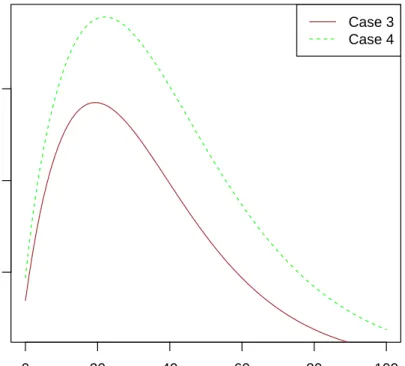
which are referred to as case 3 and 4 respectively (E[V] = 7/8 and E[Y] = 15/8 in both cases). Let us assume the premium rate c= 5/2 in both case 3 and case 4.

f(t, y) Case 3 3₄e−t 2 3e −2₃y₊1 4(2e −2t₎ 2 3 2 ye−23y Case 4 3₄e−t 2 3e −2₃y₊1 4(2e −2t₎1 3e −1₃y

Table 3.2: Joint pdf of interclaim times and claim sizes: dependent cases

As in the above independent example, the mean and variance of the time to ruin are plotted against the initial surplus in the following.

(55)

0 20 40 60 80 100 0 2 4 6 8 10 12 14 u Expected time to r uin Case 3 Case 4

(56)

0 20 40 60 80 100 500 1000 1500 u V ar

iance of the time to r

uin

Case 3 Case 4

Figure 3.4: Comparison of the variance of time to ruin in dependent cases

The observations from figure 3.3 and figure 3.4 are similar to those in the independent cases. First, in either figure 3.3 or figure 3.4, the curves are concave. Second, the curves for case 3 are below that for case 4, which may be explained by the lower variance of each increment, i.e. V ar(cV −Y), in case 3. For detailed explanation of these observations, readers can refer to the analysis in the independent cases.

(57)

Chapter 4

Laplace transform of the moments of

ruin time and analysis under Coxian

interclaim time

In the first part of this chapter, the Laplace transform of the moments of time to ruin is studied in general under dependent Sparre Andersen models. The result generalizes the properties of the Laplace transform of the Gerber-Shiu function shown in Cheung et al. (2010). In the second part, the model of Willmot and Woo (2012) is considered which assumes that the interclaim times are Coxian and the claim sizes are time-dependent. The Laplace transform of the moments of time to ruin and the function h∗k

2,δ(x, y, v|0) defined

in (2.12) are specified under this model.

(58)

4.1

Laplace transform of the moments of the time to

ruin

Assume an arbitrary dependent Sparre Andersen model introduced in Section 1.1, with the joint pdf of the interclaim time and claim size denoted byf(t, y). In this chapter, consider the Gerber-Shiu function

mδ(u) =E[e−δTw(UT−,|UT|, RNT−1)I(T < ∞)|U0 =u], (4.1)

which includes the surplus before ruin UT−, the deficit at ruin |UT| and the surplus

im-mediately after the second last claim before ruin RNT−1 in the penalty function. For

k= 0,1,2, . . ., consider the generalized kth moment of the time to ruin

mk,δ(u) =E[Tke−δTw(UT−,|UT|, RNT−1)I(T <∞)|U0 =u]. (4.2)

By definition,m0,δ(u) =mδ(u).

Cheung et al. (2010) and Willmot and Woo (2012) showed that the Laplace transform of the Gerber-Shiu function (4.1) satisfies

{1−f˜(δ−cs, s)}m˜δ(s) = ˜β0,δ(s)−σ0,0,δ(s), (4.3) where ˜ f(r, s) = Z ∞ 0 Z ∞ 0 e−rt−syf(t, y)dtdy (4.4) is the joint Laplace transform of the interclaim time and the claim size and ˜β0,δ(s) =

R∞ 0 e −su_β 0,δ(u)du with β0,δ(u) = Z ∞ 0 e−δt Z ∞ u+ct

(59)

Also, σ0,0,δ(s) = Z ∞ 0 e−sxϕ0,0,δ(x, δ−cs)dx with ϕ0,0,δ(x, h) = Z ∞ x/c e−ht Z x 0 mδ(x−y)f(t, y)dydt.

As mentioned in Cheung et al. (2010),

1−f(δ˜ −cs, s) = 0 (4.5) is Lundberg’s equation (in s).

The above result can be generalized to the Laplace transform of thekth moment of the time to ruin (4.2) for k = 0,1,2, . . ., as follows.

Theorem 4.1.1. Consider an arbitrary dependent Sparre Andersen model as introduced

in Section 1.1. The Laplace transform of (4.2) satisfies

{1−f˜(δ−cs, s)}m˜k,δ(s) = ˜βk,δ(s)+ k X r=1 k r ˜ fr(δ−cs, s) ˜mk−r,δ(s)− k X r=0 k r σk,r,δ(s), (4.6) where f˜r(δ−cs, s) = (−1)r ∂ r ∂δrf(δ˜ −cs, s) and β˜k,δ(s) = R∞ 0 e −su_β k,δ(u)du with βk,δ(u) = Z ∞ 0 tke−δt Z ∞ u+ct

w(u+ct, y−u−ct, u)f(t, y)dydt. (4.7) Also, forr = 0,1, . . . , k, σk,r,δ(s) = Z ∞ 0 e−sxϕk,r,δ(x, δ−cs)dx (4.8) with ϕk,r,δ(x, h) = Z ∞ x/c tre−ht Z x 0 mk−r,δ(x−y)f(t, y)dydt. (4.9)

(60)

Proof. To prove (4.6), rewrite (4.3) as ˜

mδ(s)−f(δ˜ −cs, s) ˜mδ(s) = ˜β0,δ(s)−σ0,0,δ(s). (4.10)

Then differentiate (4.10) k times with respect to δ, which yields

˜ mk,δ(s)− k X r=0 k r ˜ fr(δ−cs, s) ˜mk−r,δ(s) = ˜βk,δ(s)− k X r=0 k r σk,r,δ(s),

and hence (4.6) follows by rearrangement.

Note that when (4.6) equals zero, the left hand side also yields Lundberg’s equation (4.5). Thus, (4.6) is a generalization of (4.3).

4.2

Coxian interclaim time assumption

In this section, the model of Willmot and Woo (2012) is considered. It is a dependent Sparre Andersen model with the joint pdf of the interclaim time (t) and the claim size (y)

f(t, y) = m X i=1 ni X j=1 τij(t)bij(y), t, y ≥0, (4.11)

whereτij(t) is Erlang pdf, i.e.

τij(t) =

λi(λit)j−1e−λit

(j−1)! , t≥0. (4.12)

The marginal pdf of the interclaim time is k(t) = m X i=1 ni X j=1 Z ∞ 0 bij(y)dy τij(t),

(61)

which is a Coxian-npdf withn =

m

X

i=1

ni. Moreover, given (4.11), Willmot and Woo (2012)

noted that (4.5) becomes 1− m X i=1 ni X j=1 λi λi+δ−cs j ˜_b_ij_{(s) = 0.} _(4.13)

In (4.11), if bij(y) = b(y) for all i, j, then it reduces to a Sparre Andersen model with

Coxian interclaim times and time-independent claim sizes. This independent case has been considered in Li and Garrido (2005) with Gerber-Shiu function (1.4), and in Willmot and Woo (2010) with the generalized form (4.1).

4.2.1

Laplace transform of the moments

By assuming thatndistinct roots with nonnegative real parts exist for (4.13), Willmot and Woo (2012) specified the Laplace transform of the Gerber-Shiu function. The result will be generalized here to the Laplace transform to the moments of the time to ruin by the approach in Willmot and Woo (2012). In other words, the form of the Laplace transform of the moments will be determined.

Theorem 4.2.1. Consider a dependent Sparre Andersen model introduced in Section (1.1)

with joint pdf of the claim size and interclaim time given by (4.11). Furthermore, assume n

(62)

the Laplace transform of the kth moment of the time to ruin (4.2) is given by ˜ mk,δ(s) = 1 1− m X i=1 ni X j=1 λi λi+δ−cs j ˜_b ij(s) × ( ˜ βk,δ(s) + k X r=1 k r ( m X i=1 ni X j=1 λj_ij(j + 1)· · ·(j+r−1) (λi+δ−cs) j+r ˜bij(s) ) ˜ mk−r,δ(s) − k X r=0 k r σk,r,δ(s) ) , (4.14) where β˜k,δ(s) = R∞ 0 e −su_β k,δ(u)du with βk,δ(u) = Z ∞ 0 tke−δt Z ∞ u+ct w(u+ct, y−u−ct, u) ( _m X i=1 ni X j=1 τij(t)bij(y) ) dydt. (4.15) Moreover, σk,0,δ(s) = n X h=1 Qk,δ(ρh) n Y j=1,j6=h s−ρj ρh−ρj m Y i=1 (λi+δ−cs)ni , (4.16) where Qk,δ(ρh) = ( ˜ βk,δ(ρh) + k X r=1 k r ( m X i=1 ni X j=1 λj_ij(j+ 1)· · ·(j+r−1) (λi+δ−cρh)j+r ˜ bij(ρh) ) ˜ mk−r,δ(ρh) − k X r=1 k r σk,r,δ(ρh) ) _m Y x=1 (λx+δ−cρh)nx for h= 1,2, . . . , n.

Proof. First, with assumption (4.11), it follows that

˜ f(δ−cs, s) = m X i=1 ni X j=1 λi λi +δ−cs j ˜_b ij(s) (4.17)

(63)

and ˜ fr(δ−cs, s) = (−1)r ∂r ∂δr m X i=1 ni X j=1 λi λi+δ−cs j ˜_b_ij_(s) = m X i=1 ni X j=1 λj_ij(j+ 1)· · ·(j+r−1) (λi+δ−cs)j+r ˜_b ij(s). (4.18)

Substitute (4.17) and (4.18) into (4.6) gives ( 1− m X i=1 ni X j=1 λi λi+δ−cs j ˜_b ij(s) ) ˜ mk,δ(s) = ˜βk,δ(s) + k X r=1 k r ( m X i=1 ni X j=1 λj_ij(j+ 1)· · ·(j+r−1) (λi+δ−cs) j+r ˜bij(s) ) ˜ mk−r,δ(s) − k X r=0 k r σk,r,δ(s), (4.19)

which is (4.14) after rearrangement. Moreover, (4.15) follows easily from (4.7) with as-sumption (4.11).

There is still σk,0,δ(s) which needs to be determined. To start with, substitute (4.11)

into (4.9) which yields

ϕk,r,δ(x, h) = Z ∞ x/c tre−ht Z x 0 mk−r,δ(x−y) ( _m X i=1 ni X q=1 τiq(t)biq(y) ) dydt = m X i=1 ni X q=1 αk−r,δ,iq(x) Z ∞ x/c tre−htτiq(t)dt, (4.20) where αk,δ,iq(x) = Z x 0 mk,δ(x−y)biq(y)dy. (4.21)

(64)

The integral in (4.20) can be simplified as Z ∞ x/c tre−htτiq(t)dt= Z ∞ x/c tre−ht λi(λit)q−1e−λit (q−1)! dt = (q+r−1)! (q−1)! λq_i (λi+h)q+r Z ∞ x/c (λi+h)q+rtq+r−1e−(λi+h)t (q+r−1)! dt = (q+r−1)! (q−1)! λq_i (λi+h)q+r q+r−1 X j=0 (λi+h) x_c j e−(λi+h)x_c j! = (q+r−1)! (q−1)! λ q ie −(λi+h)x_c q+r X j=1 xq+r−j_(λ i+h)−j cq+r−j_(q₊_r₋_j)!,

and hence (4.20) can be rewritten as

ϕk,r,δ(x, h) = m X i=1 ni X q=1 αk−r,δ,iq(x) q+r X j=1 (q+r−1)! (q−1)! λ q ie −(λi+h)x_c x q+r−j_(λ i+h)−j cq+r−j_(q₊_r₋_j)!. (4.22)

Substitute (4.22) into (4.8), which yields

σk,r,δ(s) = Z ∞ 0 e−sx ( _m X i=1 ni X q=1 αk−r,δ,iq(x) q+r X j=1 (q+r−1)! (q−1)! λ q ie −(λi+δ−cs)x_c × x q+r−j_(λ i+δ−cs)−j cq+r−j_(q₊_r₋_j)! dx = m X i=1 ni X q=1 q+r X j=1 (q+r−1)! (q−1)! λq_i(λi +δ−cs)−j cq+r−j_(q₊_r₋_j)! Z ∞ 0 xq+r−je−λic+δxα_k₋_r,δ,iq(x)dx = m X i=1 ni X q=1 q+r X j=1 (q+r−1)! (q−1)! λq_i(λi+δ−cs)−j (−c)q+r−j_(q₊_r₋_j)!α˜ (q+r−j) k−r,δ,iq λi+δ c , (4.23) forr = 0,1, . . . , k, where ˜ α(_k,δ,iqr) (s) = Z ∞ 0 (−x)re−sxαk,δ,iq(x)dx. (4.24)

(65)

Specifically, forr = 0 in (4.23), σk,0,δ(s) = m X i=1 ni X q=1 q X j=1 λq_i(λi+δ−cs)−j (−c)q−j_(q₋_j)! α˜ (q−j) k,δ,iq λi+δ c = m X i=1 ni X j=1 (λi+δ−cs)−j ni X q=j λq_iα˜(_k,δ,iqq−j) λi+δ c (−c)q−j_(q₋_j_)! = m X i=1 ni X j=1 θij,k,δ (λi+δ−cs)j (4.25) with θij,k,δ = ni X q=j λq_iα˜(_k,δ,iqq−j) λi+δ c (−c)q−j_(q₋_j_)!.

Equivalently, (4.25) can be expressed as σk,0,δ(s) = Qk,δ(s) m Y x=1 (λx+δ−cs)nx (4.26) with Qk,δ(s) = ( _m Y x=1 (λx+δ−cs)nx ) _m X i=1 ni X j=1 θij,k,δ (λi+δ−cs)j .

Next, recall the assumption that (4.13) has n distinct roots ρ1, ρ2, . . . , ρn. For h =

1,2, . . . , n, put s=ρh in (4.19) yields σk,0,δ(ρh) = ˜βk,δ(ρh) + k X r=1 k r ( m X i=1 ni X j=1 λj_ij(j+ 1)· · ·(j +r−1) (λi+δ−cρh)j+r ˜_b_ij_(ρ_h₎ ) ˜ mk−r,δ(ρh) − k X r=1 k r σk,r,δ(ρh). (4.27)

Again, recall that σk,r,δ(ρh) actually depends on mk−r,δ(u). Therefore for r = 1,2, . . . , k,

(66)

(4.27) can be identified recursively ink, with σ0,0,δ(ρh) = ˜β0,δ(ρh). Substitute (4.27) into (4.26) gives Qk,δ(ρh) = ( ˜ βk,δ(ρh) + k X r=1 k r ( m X i=1 ni X j=1 λj_ij(j+ 1)· · ·(j+r−1) (λi+δ−cρh)j+r ˜ bij(ρh) ) ˜ mk−r,δ(ρh) − k X r=1 k r σk,r,δ(ρh) ) _m Y x=1 (λx+δ−cρh)nx. (4.28)

Since Qk,δ(s) is a polynomial with at most degree n−1, it can be expressed in Lagrange

polynomial form as Qk,δ(s) = n X h=1 Qk,δ(ρh) n Y j=1,j6=h s−ρj ρh−ρj . (4.29)

Substitute (4.29) into (4.26) results in (4.16).

On the right hand side of (4.14), it involves ˜mk−r,δ(s) and σk,r,δ(s) for r = 1,2, . . . , k.

From definition (4.8),σk,r,δ(s) is a function ofmk−r,δ(u) which can be obtained by inversion

of ˜mk−r,δ(s) in theory. Thus, (4.14) shows that ˜mk,δ(s) can be determined recursively ink.

4.2.2

Structural quantities related to the moments

Inversion of (4.14) with respect to s gives the kth moment of the time to ruin mk,δ(u),

but it is complicated to invert in general. In this section, an alternative way is provided to solve formk,δ(u). The functionh∗2k,δ(x, y, v|0) defined in (2.12) will be determined under

the Coxian interclaim time assumption, and hence mk,δ(u) can be solved recursively in k

by the defective renewal equations shown in Theorem 2.2.1.

(67)

function h∗k 2,δ(x, y, v|0) defined in (2.12) is given by h∗₂k_,δ(x, y, v|0) = n X h=1 ξh,δ ( e−ρhv_h∗k 1,δ(x, y|v) + k X r=1 k r (( m X i=1 ni X j=1 λj_ij(j+ 1)· · ·(j+r−1) (λi+δ−cρh)j+r ˜_b ij(ρh) ) × e−ρhv_h∗k−r 1,δ (x, y|v) + Z ∞ 0 e−ρhz_h∗k−r 2,δ (x, y, v|z)dz − m X i=1 ni X q=1 q+r X j=1 (q+r−1)! (q−1)! λq_i(λi+δ−cρh)−j (−c)q+r−j_(q₊_r₋_j)!γk−r,δ,iq,q+r−j,λi_c+δ(x, y, v) )) − k X r=1 k r m X i=1 ni X q=1 λq_i (q−1)!(−c)q+rγk−r,δ,iq,q+r−1,λi_c+δ(x, y, v), (4.30) where h∗k 1,δ(x, y|u) is as defined in (2.11), ξh,δ = m Y i=1 λi+δ c −ρh ni n Y j=1,j6=h (ρj −ρh) (4.31) and γk,δ,iq,r,s(x, y, v) = Z ∞ v (−a)re−sah₁∗k_,δ(x, y|v)biq(a−v)da + Z ∞ 0 Z z 0 (−z)re−szh₂∗k_,δ(x, y, v|z−a)biq(a)dadz. (4.32)

Proof. First, with definition (2.11), note that (4.7) can be written as

βk,δ(u) = Z ∞ u Z ∞ 0 w(x, y, u)h∗₁k_,δ(x, y|u)dydx (4.33) = Z ∞ 0 Z ∞ u w(x+u, y −u, u)h∗₁k_,δ(x, y|0)dydx.

(68)

For the moment of the time to ruin (4.2), Theorem 2.2.1 shows that mk,δ(u) = φδ

Z u 0

mk,δ(u−y)fδ(y)dy+vk,δ(u) (4.34)

for k = 0,1,2, . . ., where vk,δ(u) = k X j=1 k j Z u 0 mk−j,δ(u−y) Z ∞ 0 h∗_δj(x, y|0)dxdy +βk,δ(u) + Z ∞ u Z ∞ 0 Z x 0 w(x+u, y−u, v+u)h∗₂k_,δ(x, y, v|0)dvdxdy. Foru= 0, (4.34) becomes mk,δ(0) =βk,δ(0) + Z ∞ 0 Z ∞ 0 Z x 0 w(x,