July 2010, Volume 35, Issue 11. http://www.jstatsoft.org/
Introducing
COZIGAM: An
R
Package for
Unconstrained and Constrained Zero-Inflated
Generalized Additive Model Analysis
Hai Liu
Indiana University School of Medicine
Kung-Sik Chan The University of Iowa
Abstract
Zero-inflation problem is very common in ecological studies as well as other areas. Nonparametric regression with zero-inflated data may be studied via the zero-inflated gen-eralized additive model (ZIGAM), which assumes that the zero-inflated responses come from a probabilistic mixture of zero and a regular component whose distribution belongs to the 1-parameter exponential family. With the further assumption that the probability of non-zero-inflation is some monotonic function of the mean of the regular component, we propose the constrained zero-inflated generalized additive model (COZIGAM) for an-alyzing zero-inflated data. When the hypothesized constraint obtains, the new approach provides a unified framework for modeling zero-inflated data, which is more parsimonious and efficient than the unconstrained ZIGAM. We have developed anRpackageCOZIGAM which contains functions that implement an iterative algorithm for fitting ZIGAMs and COZIGAMs to zero-inflated data based on the penalized likelihood approach. Other functions included in the package are useful for model prediction and model selection. We demonstrate the use of the COZIGAM package via some simulation studies and a real application.
Keywords: EM algorithm, model selection, penalized likelihood, proportionality constraints.
1. Introduction
Generalized additive models (GAMs, Hastie and Tibshirani 1990; Wood 2006) are widely used in applied statistics, especially for modeling nonlinear effects of the covariates in sci-entific and quantitative studies. See, for instance, Ciannelli, Fauchald, Chan, Agostini, and Dingsør(2007b) and the references therein in ecological analysis. GAMs can be estimated by
maximizing the penalized likelihood which, in general, equals
L(η)−λ2J2(η), (1) whereη is the unknown regression function on the link scale, L(η) is the log-likelihood func-tional, J2(η) is some roughness penalty, and λis the smoothing parameter that controls the trade-off between the goodness-of-fit and the smoothness of the function. The estimated re-gression functions are smoothing splines under mild regularity conditions. SeeWahba(1990), Green and Silverman(1994),Wood (2000) and Gu(2002) for details on the penalized likeli-hood approach and smoothing splines.
Zero-inflated data abound in ecological studies as well as in other scientific and quantitative fields, where the data contain an excess of zero responses. The problem is known as zero-inflation. For example, fisheries trawl survey data often contain a large number of zero catches, due to the fact that fish swim in schools influenced by food availability and irregular current pattern, see Ciannelli et al. (2007b). Zero-inflated data are often analyzed via a mixture model specifying that the response variable comes from a probabilistic mixture of zero and a regular component whose distribution (referred to as the regular distribution below) belongs to the 1-parameter exponential family distribution. SeeMullahy(1986),Lambert(1992) and Heilbron(1994) for discussions in the parametric setting. Nonparametric regression analysis of zero-inflated data can be studied via the zero-inflated generalized additive model (ZIGAM) (Chiogna and Gaetan 2007), where the mean of the regular component and the probability of non-zero-inflation are each modeled as some nonparametric smooth predictors, say,sµ(T) and
sp(T) respectively withT as the covariate. An alternative approach to modeling zero-inflated data proceeds in two stages: (i) model the presence/absence pattern by a GAM and (ii) model the response given it is non-zero by another GAM (Barry and Welsh 2002). When the response variable has a continuous regular distribution, the two-stage approach is equivalent to the ZIGAM, otherwise the two approaches are generally different. In stage (ii), the two-stage approach generally specifies the conditional response distribution given it is non-zero to belong to a zero-truncated 1-parameter exponential family, and hence its fitting involves very complex link functions and variance functions. Here, we mainly focus on the ZIGAM and its constrained versions.
If the process generating the non-zero-inflated responses and the zero-inflation process con-stitute distinct mechanisms, the functional forms of the two smooth predictors sµ(T) and
sp(T) in a ZIGAM are unconstrained. However, in many ecological data, the two processes are coupled and bear some systematic relationship. For example, in trawl survey studies, zero-inflation often arises from the spatio-temporal aggregation of fish due to their schooling behavior. For such data, the probability of positive catch is positively correlated to the volume occupied by the schools of fish which generally increases with the mean (local) abundance of the fish. Therefore, in the situation involving spatio-temporally aggregated subjects, the probability of positive catch is likely a monotonic function of the mean (local) abundance of the study population. Liu and Chan (2008) considered the case of imposing a proportional-ity constraint on sµ(T) and sp(T) up to an additive constant, which leads to a constrained zero-inflated generalized additive model (COZIGAM); see below. The imposed constraint in a COZIGAM reflects the mechanistic nature of the zero-inflation process. Moreover, it promotes estimation efficiency by effectively reducing the number of model parameters. The ZIP(τ) model proposed by Lambert (1992) in the parametric Poisson regression setting is a harbinger of our new approach. Here, the proportionality constraint may be relaxed by
letting the proportionality constants be component-specific, which allows the non-zero-data generating process and the zero-inflation process to be partially coupled. This relaxation is practically important, as illustrated by the following argument. If there are several covariates, some may influence zero-inflation in one direction and the severity mean in the other: for ex-ample, in the study of cigarette consumption, age may have a positive influence on the binary event smoker/non-smoker and on the number of cigarettes consumed by a smoker ‘yesterday’. Whether the test person was ill the day before the survey may affect the number of smoked cigarettes but is irrelevant for the smoker/non-smoker event. The component-specific con-straint formulation is appropriate for modeling such situations assuming component-specific proportionality. If the latter assumption fails, then imposing component-specific porportion-ality will result in bias. On the other hand, unconstrained ZIGAM adds probably many parameters to the model required by the smooth function and decreases the accuracy of pa-rameter estimation, even though it may improve the modeling of the covariates influence on the responses. Thus, to constraint or not to constraint hinges on the trade-off between bias and variance. Below, we shall review a BIC-type model selection criterion proposed byLiu and Chan (2008) for aiding such a decision, by assessing the validity of the proportionality constraint imposed by the COZIGAM against the (unconstrained) ZIGAM. The model selec-tion approach can be readily extended for the purpose of choosing between a ZIGAM and a GAM, which we do here.
To implement the regression analysis via the ZIGAM and the COZIGAM in real applications, we have developed anR(RDevelopment Core Team 2010) packageCOZIGAM, which can be downloaded from the Comprehensive RArchive Network at http://CRAN.R-project.org/ package=COZIGAM. The purpose of this paper is to introduce the COZIGAM and describe how to use this package. The structure of this paper is as follows. We introduce the model formulation of both the constrained and unconstrained ZIGAMs, and briefly discuss the model estimation and the proposed model selection criterion in Section2. The use of theCOZIGAM package is illustrated by both Monte Carlo studies and a real data application in Section 3. We briefly conclude in Section 4.
2. Model formulation and estimation
In this section we briefly outline the model formulations of the constrained and the uncon-strained ZIGAMs, seeLiu and Chan(2008) for details. Next, we summarize a model estima-tion procedure which may involve the expectaestima-tion-maximizaestima-tion (EM) algorithm (Dempster, Laird, and Rubin 1977). Then, we will review the Bayesian model selection criterion developed byLiu and Chan(2008) for choosing between the constrained and the unconstrained ZIGAMs, and extend it for choosing between a ZIGAM and a GAM, i.e., without zero-inflation. 2.1. Model formulation
Let Y = (Y1, Y2, . . . , Yn)> be the responses and T = (T1,T2, . . . ,Tn) be the covariates
where Yi is univariate and Ti consists of m sub-vectors: Ti = (T1i, T2i, . . . , Tmi)>. Assume that given the covariates Ti = ti, Yi’s are independent. A GAM (Wood 2006, Chapter 3) relating the responseYi to the covariateti has the general form:
whereµi =E(Yi), gµ is a monotonic link function, and η is some unknown smooth function to be estimated. Assume further thatη is additive in them covariates:
η(ti) =β0+s1(t1i) +s2(t2i) +· · ·+sm(tmi), (2) where eachsj, j = 1,· · ·, m, is a centered unknown smooth function, and β0 is the intercept.
Moreover, the conditional distribution of the response variable Yi is assumed to belong to the 1-parameter exponential family, as in a generalized linear model (GLM), seeNelder and Wedderburn(1972). In particular,
Yi|ti ∼f(yi|ϑi), i= 1, . . . , n, (3) where f(yi|ϑi) is the probability density (mass) function of some 1-parameter exponential family distribution, which has the form:
f(yi|ϑi) = exp ωi(yiϑi−b(ϑi)) φ +ci(yi, φ) , (4)
where ϑi is the canonical parameter, ωi is known constant denoting the weight of the data case which is often equal to 1, andφis the dispersion parameter. GAMs can be estimated by the penalized likelihood approach, seeWood(2006, Chapter 4) for details.
Due to its flexibility, GAMs have become widely used in various fields. Unfortunately, GAMs cannot be directly applicable for regression analysis with zero-inflated data due to the excess of zeroes. Instead, nonparametric regression with zero-inflated responses may be studied via the zero-inflated generalized additive models (ZIGAMs). The ZIGAM assumes that the response variable follows a probabilistic mixture distribution of a zero atom and a regular component whose distribution belongs to the 1-parameter exponential family:
Yi|ti∼h(yi) =
0 with probability 1−pi
f(yi|ϑi) with probability pi,
(5) where the zero atom models the zero-inflation explicitly and f is defined in (4). Below we refer tof in the mixture model (5) as the regular pdf and its corresponding distribution the regular distribution, and µi = Ef(Yi) as the regular mean which is assumed to link to the covariates as given by (2). The non-zero-inflation probability pi is linked to the covariate as follows:
gp(pi) =ξ(ti), (6) where gp is another link function, for instance, the logit function, and ξ is an unknown smooth function. If η and ξ are independent (infinite-dimensional) parameters, the model is an unconstrained ZIGAM in which case zero-inflation could be caused by a mechanism different from that underlying the non-zero-inflated responses. On the other hand, if the zero-inflation process is coupled with the process generating the non-zero-inflated data, we may expect some monotonic relationship betweenη andξ. In particular, we consider the case thatξ is constrained to be a linear function of η:
ξ=α+δ·η, (7) whereα andδare two unknown coefficients. We will refer to the zero-inflated model (5) with constraint (7) as the constrained zero-inflated generalized additive model (COZIGAM).
In some cases, the non-zero-inflated data generating process and the zero-inflation process are partially coupled so that the latter process may only depend on a subset of the smooth com-ponents affecting the non-zero-inflated response. In addition, these smooth comcom-ponents may affect the zero-inflation differently. Thus, the proportionality constraint (7) in the COZIGAM may be relaxed to allow possibly different proportionality coefficients for different covariates in the zero-inflation process. Specifically, we consider the component-specific proportionality constraint:
ξ(ti) =α+δ1s1(t1i) +δ2s2(t2i) +· · ·+δmsm(tmi), (8) whereαandδ= (δ1, . . . , δm)>are unknown parameters. In constraint (8) we assign a specific
proportionality coefficient for each additive component so that different smooth components may possibly have different effects on the zero-inflation process. Furthermore, in some appli-cations, it may be desirable to fix some proportionality coefficients to be zero, which enforces that the corresponding component covariates do not affect the zero-inflation process. In Sec-tion3we will illustrate the use of theCOZIGAMpackage for fitting ZIGAMs, and COZIGAMs with both constraints (7) and (8).
2.2. Model estimation
We now briefly outline the method of penalized likelihood for estimating a COZIGAM, with constraint (7), that is proposed byLiu and Chan(2008). The method can be readily modified for estimating a COZIGAM with component-specific constraint (8) or fitting an unconstrained ZIGAM. According to the reproducing kernel Hilbert space theory, under some mild conditions and for finite sample size, we can reparametrize the infinite-dimensional parameter η by a vector parameterβ= (β0,β>1,β>2,· · · ,β>m)>, so that
sj(tji) =Xijβj, j= 1,· · · , m,
whereXij is the i-th row of the design matrix Xj of the basis functions related to thej-th smooth componentsj. Furthermore, the roughness penalty J2(sj) can often be expressed as a quadratic formβ>j Sjβj/2, whereSj is a penalty matrix, see Gu(2002) and Wood(2006). Define the binary variablesEi, i= 1, . . . , n, with
Ei=
1 ifYi 6= 0 0 ifYi = 0.
If the underlying regular exponential family distribution is continuous, for instance, Gaussian or Gamma, the penalized log-likelihood then equals
lp(α, δ,β) = n X i=1 h eilog{pif(yi|ϑi)}+ (1−ei) log (1−pi) i −1 2 m X j=1 λ2jβ>j Sjβj, (9) whereλj is the smoothing parameter associated with sj.
If the regular distribution assigns positive probability to zero, which is the case for many discrete distributions including Poisson and binomial, the penalized log-likelihood function becomes somewhat complex:
lp(α, δ,β) = n X
i=1
h
eilogpif(yi|ϑi) + (1−ei) log (1−pi+pif(0|ϑi)) i −1 2 m X j=1 λ2jβ>jSjβj. (10)
Below, a COZIGAM will be referred to as a continuous (discrete) COZIGAM if its penalized likelihood function is given by Equation 9(Equation 10). Liu and Chan(2008) proposed an iterative algorithm for maximizing (9) or (10) with respect to the parameter θ= (α, δ,β>)> for the case of known smoothing parameter, which is motivated by the Penalized Iteratively Re-weighted Least Squares (PIRLS) method (Wood 2006, p. 169) and the Penalized Quasi-Likelihood (PQL) method (see, for instance,Green 1987;Breslow and Clayton 1993). Direct maximization of (9) could be done via a modified PIRLS algorithm, and the smoothing parameter could be determined by generalized cross validation (GCV) or unbiased risk esti-mation (UBRE); seeWood(2006, Chapter 4) for further discussions about GCV and UBRE. However, for a discrete COZIGAM, direct optimization of the penalized likelihood (10) is challenging because it complicates the use of GCV or UBRE for choosing the smoothing pa-rameter. In this case, if we augment the data by the binary variablesZi, i= 1, . . . , n, which are defined by Zi = 1 ifYi ∼f(yi|ϑi) 0 ifYi ∼0, (11) the complete-data penalized log-likelihood equals
lcp(α, δ,β) = n X i=1 h zilog{pif(yi|ϑi)}+ (1−zi) log (1−pi) i −1 2 m X j=1 λ2jβ>j Sjβj,
which has the same form as (9) and can be optimized through the modified PIRLS. Note that the variableZi defined by (11) is latent so that the EM algorithm is employed for estimating a discrete COZIGAM. The covariance matrix of the estimator can be approximately computed by inverting the observed Fisher information. See Liu and Chan (2008) for details.
2.3. Model selection
In statistical analysis, one important issue is model selection or model comparison among multiple competing models. One of the widely used model selection criteria is the Bayesian information criterion (BIC, Schwarz 1978), which selects the model with maximum posterior model probability. In the Bayesian framework, the posterior probability of model Mi equals
P(Mi|D) =
P(D|Mi)P(Mi)
P(D) ,
whereP(Mi) is the prior probability of modelMi,Ddenotes the data, and
P(D) =X i
P(D|Mi)P(Mi)
is the normalizing constant. P(D|Mi) is the marginal likelihood (also known as the evidence) of the modelMi, and it equals
P(D|Mi) = Z
P(D|θ, Mi)P(θ|Mi)dθ, (12) where P(D|θ, Mi) is the likelihood of the parameter θ under the model Mi, and P(θ|Mi) is the prior probability of θ under Mi. Assume a flat prior that P(Mi) ∝ constant, the posterior model probability P(Mi|D) is proportional to the marginal likelihood P(D|Mi).
Just like the BIC, we will use the marginal likelihood as the model selection criterion that maximizes the posterior model probability, which is applicable for choosing among nested or non-nested models; see Busemeyer and Wang (2000). Preference will be given to models with larger marginal likelihoods. For the unconstrained ZIGAM and the COZIGAM, there is generally no closed-form solution for the integral on the right side of (12). Laplace method (see, for example,Tierney and Kadane 1986) is used to approximately compute the marginal likelihood.
Liu and Chan (2008) gave the following approximate formula of the logarithmic marginal likelihood for the COZIGAM:
logE≈lp(α,b bδ,βb)− K+ 2 2 logn− 1 2log H + K+ 2−B 2 log 2π+ 1 2 m X j=1 logλ2jSj+ , (13) wherebθ= (α,b δ,bβb >
)> is the maximum penalized likelihood estimator,K= dim(β),Sj+ is a
diagonal matrix of dimensionbj with all the strictly positive eigenvalues of the penalty matrix
Sj arranged in descending order on the leading diagonal,B= Pm
j=1bj, andH is the negative Hessian matrix oflp/nevaluated at bθ.
For the ZIGAM, Liu and Chan (2008) provided the following approximation: logE≈lp(βb,γb)− K+K∗ 2 logn− 1 2log H +K+K ∗−(B+B∗) 2 log 2π+ 1 2 m X j=1 logλ2jSj+ + 1 2 m∗ X j=1 logϕ2jS∗j+ ,
where the unconstrained infinite-dimensional parameter ξ (defined in Equation 6) can be reparametrized by a parameter vector γ = (γ0,γ>1,γ2>,· · · ,γ>m∗)>, (βb
>
,γb>)> is the maxi-mum penalized likelihood estimator, K∗ = dim(γ), S∗j+ of dimensionsb∗j is a diagonal ma-trix consisting of the strictly positive eigenvalues of the penalty mama-trix associated with γj,
B∗ =Pm∗ j=1b
∗
j,ϕj, j = 1,· · ·, m∗, are the smoothing parameters associated withξ, and H is the negative Hessian matrix of the normalized penalized likelihood function evaluated at the maximizer.
Here, we extend the model selection approach of Liu and Chan (2008) for assessing the presence of zero-inflation. This can be done by fitting a ZIGAM and a GAM to the data, and then compare their marginal likelihoods. Following Liu and Chan (2008), it can be shown that the logarithmic marginal likelihood of a GAM (without zero-inflation) is given by
logE≈lp(βb)− K 2 logn− 1 2log H + K−B 2 log 2π+ 1 2 m X j=1 logλ2jSj+ . (14)
Note that the difference between (13) and (14) is thatlp(α, δ,β) in (13) is the penalized log-likelihood of a COZIGAM; furthermore the COZIGAM adds two more degrees of freedom to the GAM, while lp(β) in (14) is the penalized log-likelihood of a GAM, and accordingly the negative Hessian matrices in the two formulas are different. A higher marginal likelihood from the ZIGAM would indicate that there is zero-inflation in the count data. Otherwise, fitting the data by a GAM instead of a ZIGAM is appropriate.
3. The
COZIGAM
package
TheRpackageCOZIGAMfacilitates the fitting of a ZIGAM or a COZIGAM to zero-inflated data. It requires the installation of themgcvpackage (Wood 2008) whose magic()function is made use of in the implementation of the maximum penalized likelihood estimation algo-rithm. Some features of the mgcv package are also shared by the COZIGAM package. In this section, we illustrate the use of the COZIGAM package. First we demonstrate the use by fitting discrete COZIGAMs to simulated data. Then a real data analysis will be studied where the response variable follows a zero-inflated lognormal distribution. The main function for fitting a COZIGAM is cozigam(), which calls the COZIGAM.dis() or PCOZIGAM.dis()
function (depending on the type of constraint imposed) if it is a discrete COZIGAM.
Other-wiseCOZIGAM.cts()orPCOZIGAM.cts()function is used for model estimation of continuous
COZIGAMs. Similarly, the zigam() function which calls ZIGAM.dis() or ZIGAM.cts() is used for fitting a ZIGAM. Some other useful functions including visualizing and summarizing a fitted COZIGAM will be discussed. In addition, the model selection criterion for choosing between an unconstrained ZIGAM and a COZIGAM will be illustrated. The keyRcommands as well as outputs will be provided with associated graphics. All numerical illustrations re-ported below were computed using a PC with a CPU of 2.40×2 GHz and 3 GB RAM. Several alternativeRpackages are available for fitting various models with zero-inflated data. For example, gamlss (Stasinopoulos and Rigby 2007) fits a GAM with zero-inflated data based on a different model framework; pscl (Zeileis, Kleiber, and Jackman 2008) provides standard parametric hurdle and zero-inflated model fitting;MCMCglmm(Hadfield 2010) uses a Bayesian approach for estimating mixed models, including functionality for zero-inflated Poisson data. Further information about these models and their R implementations can be found in these references.
3.1. Simulated data
The simulations are based on two test functions, denoted bys1 and s2, which are taken from
Wood (2006, p. 197). The test function s1 has a 1-dimensional argument, while s2 has a
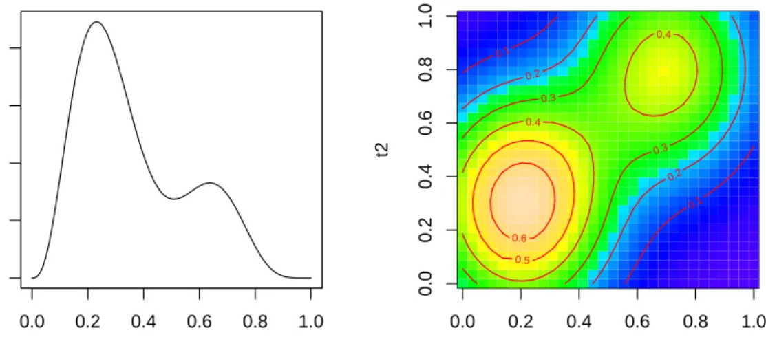
2-dimensional argument (see Figure1).
s1(t) = 0.2t11(10(1−t))6+ 10(10t)3(1−t)10, 0≤t≤1 s2(t1, t2) = 0.3×0.4π n 1.2e−(t1−0.2)2/0.32−(t2−0.3)2+ 0.8e−(t1−0.7)2/0.32−(t2−0.8)2/0.42 o , 0≤t1, t2 ≤1.
In theCOZIGAM package, the two test functions are named f0 and test respectively. We will simulate some Poisson and binomial count data based on these functions and then use the simulated data to fit COZIGAMs and ZIGAMs. As mentioned earlier, because the underlying regular distributions in these examples are discrete, the EM algorithm is used to find the maximizer of the penalized log-likelihood function (10), with initial valuesµ[0]i = max(yi,0.01),
p[0]i = 0.7 for all i= 1,· · ·, n, and α[0]= 0, δ[0] =1. Example 1: Zero-inflated Poisson data
The first example is a constrained zero-inflated Poisson model with the regular mean response given byµi = exp(η0(ti)), where η0(ti) =s1(t1i)/5 + 2s2(t2i, t3i), and the non-zero-inflation
0.0 0.2 0.4 0.6 0.8 1.0 0 2 4 6 8 s1(t) t 0.0 0.2 0.4 0.6 0.8 1.0 0.0 0.2 0.4 0.6 0.8 1.0 s2(t1,t2) t1 t2 0.1 0.1 0.2 0.2 0.3 0.3 0.4 0.4 0.5 0.6
Figure 1: Test functions used in simulation studies.
probability given by pi = logit−1{α0+δ0η0(ti)}, where α0 = −0.5, δ0 = 1.0; the covariate
(T1, T2, T3) is assumed to be independent and uniformly distributed over [0,1]3. Data from
this model can be simulated in steps. In an R session, the following set of codes loads the COZIGAMpackage and generates 500 cases of covariate values.
R> library("COZIGAM") R> set.seed(8) R> n <- 500 R> t1 <- runif(n, 0, 1) R> t2 <- runif(n, 0, 1) R> t3 <- runif(n, 0, 1)
Next, we simulate the latent Poisson count data without zero-inflation: R> eta0 <- f0(t1) / 5 + 2 * test(t2, t3)
R> mu0 <- exp(eta0)
R> y <- rpois(rep(1, n), mu0)
Finally, the Poisson variates are then set to zero with probability 1−pi. The zero-inflated Poisson data may be saved in a data frame, say nameddata1:
R> alpha0 <- -0.5 R> delta0 <- 1.0
R> p0 <- .Call("logit_linkinv", alpha0 + delta0 * eta0, PACKAGE = "stats") R> z <- rbinom(rep(1,n), 1, p0)
R> y[z == 0] <- 0
y Frequency 0 5 10 15 20 0 50 100 150 200 250
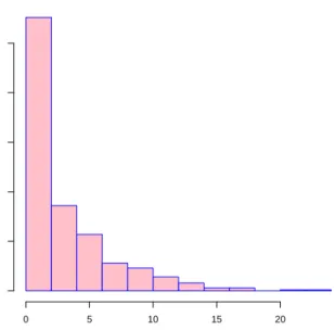
Figure 2: Histogram of the simulated zero-inflated Poisson responses.
Note that in the process of simulating the data, we actually have the information of the latent indicator variableZi (defined by Equation11). However, in model fitting, we will not use this information but treat theZi’s as missing.
The simulated zero-inflated dataset comprises of 200 zero responses out of 500 observations (40%), see Figure2. Among the 200 zero responses, some are due to zero-inflation and the rest are the zero realizations of the Poisson distribution (and we cannot tell them apart). To fit a COZIGAM to the simulated zero-inflated Poisson data, simply call the cozigam()
function in theCOZIGAM package:
R> res1 <- cozigam(y ~ s(t1) + s(t2,t3), constraint = "proportional", + conv.crit.out = 1e-3, family = poisson, data = data1)
iteration = 2 norm = 0.9125572 iteration = 3 norm = 0.4334777 iteration = 4 norm = 0.3359116 iteration = 5 norm = 0.3083645 iteration = 6 norm = 0.2004221 iteration = 7 norm = 0.1152472 iteration = 8 norm = 0.06296885 iteration = 9 norm = 0.03366744 iteration = 10 norm = 0.01782503 iteration = 11 norm = 0.009393632 iteration = 12 norm = 0.004939645 iteration = 13 norm = 0.00259332
iteration = 14 norm = 0.001360528 iteration = 15 norm = 0.0007138289 ========================================== estimated alpha = -0.4963178 ( 0.3005424 ) estimated delta = 0.8134658 ( 0.2017702 ) ==========================================
Here y ~ s(t1,t2)+s(t3) is a GAM formula (see the gam() function in the mgcv
pack-age) specifying the response and predictor variables structure; the argument constraint
= "proportional" specifies the proportionality constraint (7); conv.crit.out is the
pre-selected stopping criterion for the iterative estimation procedure (see below); the distribution of the regular component (the non-zero-inflated data) is specified via the argumentfamily, which is similar to the family argument of theglm() function for fitting a GLM; the data
argument points to the dataset where the responses and covariates are saved. For a full list of the arguments as well as the object returned by thecozigam()function, see its help manual by running the command?cozigam.
At the end of each iteration, the iteration number and the maximum norm of the difference between the current estimate and the previous one is displayed on the console, which lets the user keep track of the progress of the estimation procedure. The maximum norm is defined as norm= max |αb−αbold|,|bδ−bδold| ,
where α,b δb are the current parameter estimates and αbold,bδold are the estimates from the previous iteration. The iteration procedure is considered to have successfully converged if the maximum norm is sufficiently small, i.e., it is less than the value specified by the
argu-mentconv.crit.out, at which iterate the estimation algorithm stops. For this example, the
estimation algorithm converged after 15 iterations which took less than 10 seconds. Further-more, the function outputs the parameter estimatesα,b bδ, with their standard errors enclosed in parentheses. The generic function summary() presents further useful information about the fitted COZIGAM:
R> summary(res1)
Family: poisson Link function: log Formula:
y ~ s(t1) + s(t2, t3) Parametric coefficients:
Estimate Std. Error z value Pr(>|z|)
(Intercept) 1.31622 0.03636 36.198 < 2e-16 ***
alpha -0.49632 0.30054 -1.651 0.0987 .
delta1 0.81347 0.20177 4.032 5.54e-05 ***
Approximate significance of smooth terms: edf Est.rank Chi.sq p-value
s(t1) 7.435 9 377.2 <2e-16 ***
s(t2,t3) 11.744 24 132.9 <2e-16 ***
---Signif. codes: 0 `***' 0.001 `**' 0.01 `*' 0.05 `.' 0.1 ` ' 1
Scale est. = 1 n = 500
The above summary consists of two parts: the first part reports the parametric estimation results which includes the estimate of the intercept term β0 in (2), as well as those of the
constraint parameters α andδ. The corresponding standard errors of the estimators and the Wald test results for testing whether the parameters are individually equal to 0 are also given. The second part reports the estimation results of the nonparametric smooth components, which lists the efficient degrees of freedom (edf) for each smooth term and the approximate F tests for significance. See Wood (2006) for relevant discussions in the context of GAM. The last line in the summary reports the scale (dispersion) parameter estimate of the regular distribution or its true value (if it is known), and the sample size as well; for example, the scale parameter is known and equals 1 for Poisson distributions. The users can check the help manual on the object returned by the cozigam() function (in this example saved as res1) for more information of the fitted COZIGAM.
The smooth function estimates can be displayed using the generic function plot(). The commands
R> par(mfrow = c(1, 2))
R> plot(res1, shade.ci = TRUE, Rug = TRUE)
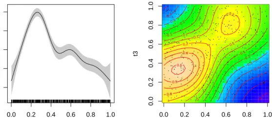
produce two figures, one for each of two smooth components in the modelres1, as shown in Figure3. The plotting convention depends on the dimension of the argument of the function. For the case of 1-dimensional argument, the function estimate is plotted as a smooth function by connecting the point estimates over a grid by lines in the plot, with a 95% pointwise confidence band. Setting the argumentshade.citoTRUE shades the confidence band in grey but otherwise the confidence band is unshaded except that its upper and lower boundaries are drawn as dashed lines. The covariate values of each data case are drawn as a short stick on the bottom of the x-axis if Rug = TRUE.
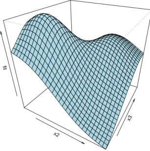
For the 2-dimensional case, the function estimate is displayed in a contour plot by default, with the covariate values of each data case plotted as a dot ifRug = TRUE(the right panel of Figure3). Alternatively, the function estimate can be drawn in a perspective plot by setting the argumentplot.2d = "persp". We could also require only the second smooth component
s2 to be plotted by letting select = 2. The command to produce Figure 4 is listed below.
Note that the test functions are scaled in the model and the estimated smooth functions are centered at 0.
0.0 0.2 0.4 0.6 0.8 1.0 −1.0 −0.5 0.0 0.5 1.0 t1 0.0 0.2 0.4 0.6 0.8 1.0 0.0 0.2 0.4 0.6 0.8 1.0 t2 t3 −0.7 −0.6 −0.5 −0.4 −0.4 −0.3 −0.3 −0.2 −0.2 −0.1 −0.1 0 0 0.1 0.1 0.2 0.2 0.3 0.4 0.5 0.6
Figure 3: Plots of fitted smooth functions in Example 1. The left panel depicts the estimate ofs1, and the right panel displays the estimated s2.
Given a new set of covariates, we can use the generic functionpredict()to make predictions for the new data. Suppose we have two new observations with predictors ˜t1 = (0.5,0.2,0.3)>
and ˜t2 = (0.8,0.1,0.7)>. To predict the response values at those two points, we first create a
data frame named newdata containing the new data:
R> newdata <- data.frame(t1 = c(0.5, 0.8), t2 = c(0.2, 0.1), + t3 = c(0.3, 0.7)) R> newdata t1 t2 t3 1 0.5 0.2 0.3 2 0.8 0.1 0.7
The names of the covariates in the new data set must match those in the fitted model. In the case of missing values in the covariate or if there is a mis-match in the covariate names,
the predict() function will return an error message. Next, we call the function predict()
to make predictions for the new observations:
R> pred <- predict(res1, newdata = newdata, se.fit = TRUE, type = "response") R> pred
fit se p
1 6.112847 0.6563248 0.7263883 2 2.327128 0.2841570 0.5475469
x2
x3 fit
Figure 4: Perspective plot of the estimateds2(t2, t3) in Example 1.
With the option se.fit = TRUE, the standard errors of the point predictors are computed and reported in the output. The argument type = "response" specifies that predictions are done on the original scale of the response, whereas if type = "link", predictions on the link scale are returned. The returned object is a data frame that consists of three columns: the column fit gives the predicted response for each observation; the column se gives the standard errors of the point predictors; and the last columnp gives the predicted non-zero-inflation probability.
Example 2: Zero-inflated binomial data
In the second example, we fit a zero-inflated binomial model with the component-specific constraint (8). We first generate the latent binomial count data with probability of success
µ0(ti) = logit−1{¯s1(t1i)/5 + 3¯s2(t2i, t3i)−0.6}, where ¯sdenotes the function centered over the sampling points andN is the number of trials:
R> set.seed(23) R> n <- 800 R> N <- as.integer(runif(n, 3, 11)) R> t1 <- runif(n, 0, 1) R> t2 <- runif(n, 0, 1) R> t3 <- runif(n, 0, 1) R> eta.p10 <- (f0(t1) - mean(f0(t1)))/5
R> eta.p20 <- (test(t2, t3) - mean(test(t2, t3))) * 3 R> eta0 <- eta.p10 + eta.p20 - 0.6
R> mu0 <- binomial()$linkinv(eta0) R> y <- rbinom(n, N, mu0)
Then the binomial responses are set to zero with probability 1−pi, wherepi = logit−1{0.8 + 1.2¯s1(t1i)}, i.e., the true constraint coeffients are α0= 0.8, δ10= 1.2 andδ20= 0:
R> alpha0 <- 0.8 R> delta10 <- 1.2 R> delta20 <- 0
R> p0 <- .Call("logit_linkinv", alpha0 + delta10*eta.p10 + delta20 * eta.p20, + PACKAGE = "stats")
R> z <- rbinom(p0, 1, p0) R> y[z == 0] <- 0
R> data2 <- data.frame(y = y, t1 = t1, t2 = t2, t3 = t3, N = N)
Note that in this example the zero-inflation process is in fact partially coupled with the regular binomial data generating process, because we set δ20 = 0 so that the
non-zero-inflation probability only depends on the first smooth component s(t1). We can fit a
CO-ZIGAM with component-specific constraint to the data by setting the argumentconstraint
= "component" in the cozigam()function:
R> res2 <- cozigam(y/N ~ s(t1) + s(t2,t3), constraint = "component",
zero.delta = c(NA, NA), size = data2$N, family = binomial, data = data2)
iteration = 2 norm = 2.024079 iteration = 3 norm = 0.5581407 iteration = 4 norm = 0.3056323 iteration = 5 norm = 0.1603028 iteration = 6 norm = 0.1344999 iteration = 7 norm = 0.1180119 iteration = 8 norm = 0.0928619 iteration = 9 norm = 0.06900769 iteration = 10 norm = 0.04951595 iteration = 11 norm = 0.03471060 iteration = 12 norm = 0.02394276 iteration = 13 norm = 0.01632966 iteration = 14 norm = 0.01104894 iteration = 15 norm = 0.007433903 iteration = 16 norm = 0.004981663 iteration = 17 norm = 0.003328833 iteration = 18 norm = 0.002219848 iteration = 19 norm = 0.001478151 iteration = 20 norm = 0.0009832362 ==========================================
estimated alpha = 0.740801 ( 0.09779283 ) estimated delta1 = 1.287182 ( 0.2679535 ) estimated delta2 = -0.02485902 ( 0.2285234 ) ==========================================
The argumentzero.deltacan be used to fix some proportionality coefficients to be 0 in order to exclude the corresponding covariates (smooth components) from the zero-inflation process. For example, if the model has two smooth componentss(t1i) ands(t2i),zero.delta = c(NA, 0) would include only the first smooth component in the zero-inflation constraint, so that,
gp(pi) = α+δ1s(t1i). In the above example, we initially did not fix δ2, but let the data tell
us which covariate may affect the zero-inflation process, as, in practice, there may be little information on which factors affects zero-inflation. Instead, we fitted a COZIGAM with all constraint coefficients being free parameters. The fitted model yields that δb2 =−0.025 with standard error 0.229, which is not significant. Hence, we fitted another COZIGAM with δ2
fixed to be 0 (unreported). In practice we can use similar strategy or some prior information to determine which smooth components should be included in the zero-inflation constraint.
The use of model selection criterion
In Section2we have discussed the proposed model selection criterion for choosing between an unconstrained ZIGAM and a COZIGAM. We demonstrate its use here. Let us revisit the first example with zero-inflated Poisson responses. We have fitted a COZIGAM with the fitted model saved as res1. The validity of the proportionality constraint (7) can be checked via model comparison between the fitted COZIGAM and an unconstrained ZIGAM, the latter of which can be fitted by the zigam()function:
0.0 0.2 0.4 0.6 0.8 1.0 −1.5 −1.0 −0.5 0.0 0.5 1.0 t1 0.0 0.2 0.4 0.6 0.8 1.0 0.0 0.2 0.4 0.6 0.8 1.0 t2 t3 0.1 0.2 0.2 0.2 0.3 0.3 0.4 0.5 0.6 0.7
Figure 5: Plots of the smooth function components of the non-zero-inflation probability, on the logit scale, of the fitted ZIGAM with the data of Example 1. The left panel depicts the estimate ofs1, and the right panel displays the estimated s2.
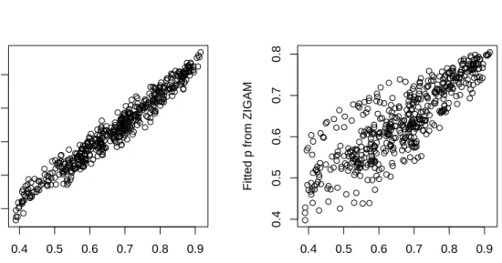
0.4 0.5 0.6 0.7 0.8 0.9 0.4 0.5 0.6 0.7 0.8 p0
Fitted p from COZIGAM
0.4 0.5 0.6 0.7 0.8 0.9 0.4 0.5 0.6 0.7 0.8 p0
Fitted p from ZIGAM
Figure 6: Plots of fitted non-zero-inflation probabilities vs. the true from both the COZIGAM (left) and ZIGAM (right).
R> res1.un <- zigam(y ~ s(t1) + s(t2,t3), family = poisson, data = data1) We can then compare the (approximate) logarithmic marginal likelihoods of the two models: R> res1$logE; res1.un$logE
[1] -962.3233 [1] -969.3942
The COZIGAM has a greater marginal likelihood (−962.32) than the unconstrained ZIGAM (−969.39), which suggests that the more parsimonious COZIGAM is preferred by the model selection criterion. It is instructive to compare the non-zero-probability functions from the two model fits. Because the ZIGAM assumes no constraint on the smooth function of non-zero-inflation probability ξ, its estimated smooth components have much wider confidence intervals (Figure 3) as compared to their counterparts of the COZIGAM (Figure3). Figure6 plots the estimated non-zero-inflation probabilities versus their true counterpart with the left diagram for the fitted COZIGAM and the right digram for the fitted (unconstrained) ZIGAM, which shows that the ZIGAM results in much more variable estimates than the COZIGAM. The larger variablility in the ZIGAM estimates owes to the fact that the ZIGAM estimate of the non-zero-inflation probability function is based on the presence/absence binary data, which is generally less informative than the non-zero-inflated data. This confirms that fitting a COZIGAM gains efficiency when the constraint obtains (Liu and Chan 2008).
Furthermore, we can use the model selection criterion to check the presence of zero-inflation. The function disgam() can be used to fit discrete GAMs and calculate their corresponding logarithmic marginal likelihoods:
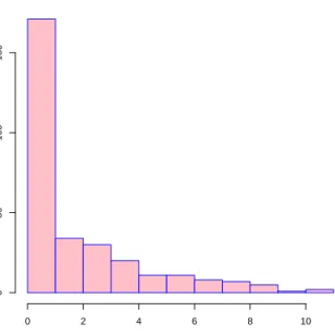
y Frequency 0 2 4 6 8 10 0 50 100 150
Figure 7: Histogram of the simulated non-zero-inflated Poisson responses. R> res1.gam <- disgam(y ~ s(t1) + s(t2,t3), family = poisson, data = data1) R> res1.gam$logE
[1] -1245.787
The logarithmic marginal likelihood of the fitted GAM (−1245.79) which does not incorporate zero-inflation is much lower than that of the (unconstrained) ZIGAM model, revealing the presence of zero-inflation.
Consider another example in which we simulated Poisson data that are not zero-inflated and the Poisson mean equals exp{s1(t1)/3−1} with sample size n = 300. The simulated
Poisson responses have 98 zeroes. The histogram of the non-zero-inflated Poisson responses in Figure 7 looks very similar to Figure 2 where zero-inflation does exist. Therefore, in this case, we cannot easily tell whether zero-inflation is present in the data. However, the model selection approach provides a convenient way to assessing the presence of zero-inflation. The Poisson data were generated by the following Rcodes:
R> set.seed(1) R> n <- 300 R> t1 <- runif(n, 0, 1) R> eta0 <- f0(t1)/3 - 1 R> mu0 <- exp(eta0) R> y <- rpois(rep(1, n), mu0) R> data3 <- data.frame(y = y, t1 = t1)
We fitted a GAM and a ZIGAM to the data respectively and then compared their logarithmic marginal likelihoods:
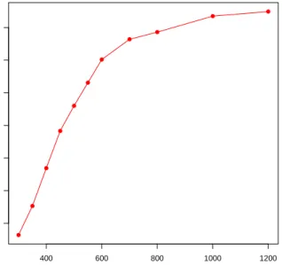
400 600 800 1000 1200 0.3 0.4 0.5 0.6 0.7 0.8 0.9 Sample Size Proportion
Figure 8: Proportions of choosing the true model under different sample sizes. The simulation results are based on 1000 replications for each case.
R> res3.gam <- disgam(y ~ s(t1), family = poisson, data = data3) R> res3.un <- zigam(y ~ s(t1), family = poisson, data = data3) R> res3.gam$logE; res3.un$logE
[1] -460.9531 [1] -476.6719
The higher logarithmic marginal likelihood of the fitted GAM (−460.95) suggests that there is no zero-inflation in the data.
We could also compare the marginal likelihood of a GAM with that of a COZIGAM for checking the presence for zero-inflation. However, because the COZIGAM adds only two more degrees of freedom to the parameter space, the model selection criterion tends to choose the COZIGAM over the GAM even though the true model is non-zero-inflated, for relatively small sample size. We study the relative frequency of detecting the presence of zero-inflation by choosing between a GAM and a COZIGAM, via simulations using the above model setting and with different sample sizes. The simulation results are summarized in Figure 8, which suggests that, for small to medium sample sizes, the model selection criterion is not so powerful in picking the true (non-zero-inflated) model. However, for large sample sizes, the proportion of choosing the true model increases from 80.2% when n = 600 to 94.5% when n = 1200. On the other hand, our limited simulation experience suggests that if the model comparison is restricted to between the GAM and the ZIGAM, the model selection approach was found to yield very high probability (above 90%) of choosing the true model even with relatively small sample size (e.g.,n= 200), whether the true model is zero-inflated or not. Therefore, in order to use the model selection approach to detect zero-inflation in the data, our suggestion
is to compare the marginal likelihood of the GAM with that of the (unconstrained) ZIGAM, unless the sample size is sufficiently large, in which case we can also compare the GAM with the COZIGAM.
3.2. Real data application
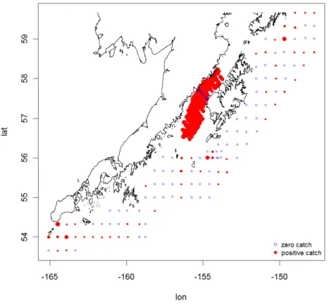
Now we illustrate the use of the COZIGAM package with a real data application; see Liu and Chan (2008) for further discussion. The data analyzed in this example is part of an extensive survey data on walleye pollock egg density (numbers 10m−2) collected during the ichthyoplankton surveys of the Alaska Fisheries Science Center (AFSC, Seattle) in the Gulf of Alaska (GOA) from 1972 to 2000. Ciannelli, Bailey, Chan, and Stenseth(2007a) showed that the spatial-temporal distribution of the pollock egg in the GOA underwent a change around 1989–90. However, their analysis was confined to positive catch data and information from the zero catches were ignored. Here, we illustrate the use of the COZIGAM for extracting information from all data including zero catches. For simplicity, we only analyze the data from 1987 which contain 274 observations sampled from the 93rd to the 116th Julian day over sites with bottom depth in the range of 28–5200m. This dataset is included in theCOZIGAM package with nameeggdata.
Figure 9: Raw data plot of pollock egg density. Blue circles denote zero catches; positive catches are displayed by red dots, whose sizes are proportional to logarithmic responses.
To load the dataset into anRsession, type R> data("eggdata")
The first 6 observations are all zero catches: R> head(eggdata)
bottom lon lat catch j.day year
1 170 -147.7500 59.33333 0 99 1987 2 620 -147.7500 59.01333 0 100 1987 3 160 -148.3000 59.03333 0 100 1987 4 135 -148.3167 59.35000 0 100 1987 5 175 -149.0000 59.00000 0 101 1987 6 115 -149.0333 58.33333 0 101 1987
The dataset contains six variables: bottom records the bottom depth (in meters) for each observation;lonand latrepresent longitude and latitude respectively, i.e., the geographical location of each sampling site; thecatchcolumn contains the observed pollock egg abundance which is measured by CPUE (catch per unit effort);j.dayis the Julian day information; and the last variable is year.
There are totally 274 observations in the year of 1987, among which 84 are zero catches making up over 30% of the data (see Figure9). Because the survey in 1987 took place in a relatively short period (93rd to 116th Julian day), preliminary analysis showed that the sampling day is not significant and hence it could be dropped from the analysis. Here, the main goal is to explore the spatial distribution of pollock spawning aggregations in the GOA. The response variable is the CPUE, and the covariates include location (longitude and latitude) and (log-transformed) bottom depth. Consider the model that the CPUE follows a COZIGAM with a zero-inflated lognormal distribution. Specifically, for thei-th observation, i= 1, . . . ,274,
CPUEi|ti ∼
0 with probability 1−pi Lognormal(µi, σ2) with probability pi.
The mean response µi of the (log) non-zero-inflated data is assumed to be additive in the covariates:
µi =β0+s(loni,lati) +s(log(bottomi)), (15) with the following constraint on the non-zero-inflation probabilitypi:
logit(pi) =α+δ·µi, (16) where β0, α, δ are parameters, s are assumed to be distinct smooth functions if they have
distinct arguments; for model identifiability, the smooth functions are constrained to be of zero mean and hence the corresponding function estimates are centered over the data. The function cozigam() was called to fit a COZIGAM to the pollock egg data: R> egg.res <- cozigam(catch ~ s(lon, lat) + s(log(bottom)),
iteration = 2 norm = 1.665588 iteration = 3 norm = 0.1355504 iteration = 4 norm = 0.01318743 iteration = 5 norm = 0.001327496 iteration = 6 norm = 0.0001342566 ========================================== estimated alpha = -1.815788 ( 0.3471865 ) estimated delta = 0.4894744 ( 0.0635757 ) ==========================================
The argument log.tran = TRUE effects the log-transformation to all positive responses so that the normal family is specified in the model fit.
Before accepting the fitted COZIGAM, we need to assess the validity of the contraint on the non-zero-inflation probability. We do this by fitting an unconstrained ZIGAM to the data and comparing its logarithmic marginal likelihood with that of the COZIGAM:
R> egg.res.un <- zigam(catch ~ s(lon,lat) + s(log(bottom)), + log.tran = TRUE, family = gaussian, data = eggdata) R> egg.res$logE; egg.res.un$logE
[1] -454.6639 [1] -463.1898
which provides some justification for constraining the non-zero-inflation probability specified by (16). The fitted model is summarized as follows:
R> summary(egg.res)
Family: gaussian
Link function: identity Formula:
catch ~ s(lon, lat) + s(log(bottom)) Parametric coefficients:
Estimate Std. Error t value Pr(>|t|)
(Intercept) 6.26022 0.10811 57.904 < 2e-16 ***
alpha -1.81579 0.34719 -5.230 3.64e-07 ***
delta1 0.48947 0.06358 7.699 3.39e-13 ***
---Signif. codes: 0 `***' 0.001 `**' 0.01 `*' 0.05 `.' 0.1 ` ' 1
Approximate significance of smooth terms:
edf Est.rank F p-value
s(lon,lat) 24.067 29 13.971 < 2e-16 ***
Figure 10: Effects of location and bottom depth: The left diagram shows the contour plot of
s(lon,lat) on the right side of Equation15; the right diagram depicts the bottom depth effect
s(log(bottom)) with 95% pointwise confidence band.
−3 −2 −1 0 1 2 3 −3 −2 −1 0 1 2 3 Theoretical Quantiles Sample Quantiles 2 4 6 8 10 −3 −2 −1 0 1 2 3 Fitted Residuals 2 4 6 8 10 2 4 6 8 10 Fitted Responses
Figure 11: Model diagnostics based on the non-zero pollock egg data.
---Signif. codes: 0 `***' 0.001 `**' 0.01 `*' 0.05 `.' 0.1 ` ' 1
Scale est. = 1.0723 n = 274
The parameter estimates for Equation 16 are αb = −1.816 (0.347) and δb = 0.489 (0.064), which is significantly positive. Recall the non-zero-inflation probability p is the probability of positive catch. Because logit(p) = α+δµ,bδ >0 implies that less egg density (smaller µ) will result in less positive catch (smaller p), and hence more zero-inflation. Thus, there is strong evidence indicating that zero-inflation is more likely to occur at locations with less egg
density. Approximate F tests show that the two smooth functions are highly significant. See Figure 10 for the plots of the estimated functions.
The validity of the lognormal regression assumption for the positive data may be explored with the model fit using only the residuals of the non-zero data. The model diagnostic plots including the Q-Q normal score plot of the residuals and the plot of residuals vs. fitted values (Figure 11) suggest that the model assumptions for the positive data are generally valid. Therefore the lognormal regression assumption is reasonable according to the model diagnostics.
4. Conclusion
In summary, we have presented a new approach for analyzing zero-inflated data, and intro-duced a corresponding package COZIGAM of R routines for fitting constrained and uncon-strained zero-inflated generalized additive models. Some simulation studies and a real data application were used to illustrate the use of the COZIGAM package. Future work includes incorporating more general form of constraints on the non-zero-inflation probability, develop-ing methods of model diagnostics for zero-inflated models usdevelop-ing all data, and extenddevelop-ing the package to fit threshold COZIGAM that can account for nonstationarity or nonlinearity. We plan to incorporate some of these features into later versions of the COZIGAMpackage.
Acknowledgments
We thank an Associate Editor and two referees for helpful comments and suggestions including the cigarette consumption example. We gratefully acknowledge partial support from the US National Science Foundation (CMG-0620789) and North Pacific Research Board (Project 709; Publication No. 217).
References
Barry SC, Welsh AH (2002). “Generalized Additive Modelling and Zero Inflated Count Data.” Ecological Modelling,157(2-3), 179–188.
Breslow NE, Clayton DG (1993). “Approximate Inference in Generalized Linear Mixed Mod-els.”Journal of the American Statistical Association,88(421), 9–25.
Busemeyer JR, Wang YM (2000). “Model Comparisons and Model Selections Based on Gen-eralization Criterion Methodology.”Journal of Mathematical Psychology,44, 171–189. Chiogna M, Gaetan C (2007). “Semiparametric Zero-Inflated Poisson Models with Application
to Animal Abundance Studies.”Environmetrics,18, 303–314.
Ciannelli L, Bailey K, Chan KS, Stenseth NC (2007a). “Phenological and Geographical Pat-terns of Walleye Pollock Spawning in the Gulf of Alaska.” Canadian Journal of Aquatic and Fisheries Sciences,64, 713–722.
Ciannelli L, Fauchald P, Chan KS, Agostini VN, Dingsør GE (2007b). “Spatial Fisheries Ecology: Recent Progress and Future Prospects.”Journal of Marine Systems,71, 223–236.
Dempster AP, Laird NM, Rubin DB (1977). “Maximum Likelihood from Incomplete Data via the EM Algorithm (with Discussion).”Journal of the Royal Statistical Society B,39, 1–38. Green PJ (1987). “Penalized Likelihood for General Semi-Parametric Regression Models.”
International Statistical Review,55, 245–259.
Green PJ, Silverman BW (1994). Nonparametric Regression and Generalized Linear Models. Chapman and Hall, London.
Gu C (2002). Smoothing Spline ANOVA Models. Springer-Verlag, New York.
Hadfield JD (2010). “MCMC Methods for Multi-Response Generalized Linear Mixed Models: The MCMCglmm R Package.” Journal of Statistical Software, 33(2), 1–22. URL http: //www.jstatsoft.org/v33/i02/.
Hastie TJ, Tibshirani RJ (1990). Generalized Additive Models. Chapman and Hall, London. Heilbron D (1994). “Zero-Altered and Other Regression Models for Count Data with Added
Zeros.”Biometrical Journal,36, 531–547.
Lambert D (1992). “Zero-Inflated Poisson Regression, with an Application to Defects in Manufacturing.”Technometrics,34(1), 1–14.
Liu H, Chan KS (2008). “Constrained Generalized Additive Model with Zero-Inflated Data.” Technical Report 388, The University of Iowa, Department of Statistics and Actuarial Sci-ence.
Mullahy J (1986). “Specification and Testing of Some Modified Count Data Models.”Journal of Econometrics,33, 341–365.
Nelder JA, Wedderburn RWM (1972). “Generalized Linear Models.” Journal of the Royal Statistical Society A,135, 370–384.
RDevelopment Core Team (2010).R: A Language and Environment for Statistical Computing. Vienna, Austria. ISBN 3-900051-07-0, URL http://www.R-project.org/.
Schwarz G (1978). “Estimating the Dimension of a Model.” The Annals of Statistics, 6(2), 461–464.
Stasinopoulos DM, Rigby RA (2007). “Generalized Additive Models for Location Scale and Shape (GAMLSS) in R.” Journal of Statistical Software, 23(7), 1–46. URL http://www. jstatsoft.org/v23/i07/.
Tierney L, Kadane JB (1986). “Accurate Approximations for Posterior Moments and Marginal Densities.”Journal of the American Statistical Association,18(393), 82–86.
Wahba G (1990). Spline Models for Observational Data. Volume 59 of CBMS-NSF Regional Conference Series in Applied Mathematics, Philadelphia, SIAM.
Wood SN (2000). “Modelling and Smoothing Parameter Estimation with Multiple Quadratic Penalties.”Journal of the Royal Statistical Society B,62, 413–428.
Wood SN (2006). Generalized Additive Models: An Introduction with R. Chapman and Hall, London.
Wood SN (2008). mgcv: GAMs with GCV Smoothness Estimation and GAMMs by REML/PQL. R package version 1.3-31, URL http://CRAN.R-project.org/package= mgcv.
Zeileis A, Kleiber C, Jackman S (2008). “Regression Models for Count Data in R.” Journal of Statistical Software,27(8), 1–25. URL http://www.jstatsoft.org/v27/i08/.
Affiliation: Hai Liu
Division of Biostatistics
Indiana University School of Medicine
Indianapolis, IN 46202, United States of America E-mail: [email protected]
URL: http://www.biostat.iupui.edu/Faculty/HaiLiu.aspx Kung-Sik Chan
Department of Statistics and Actuarial Science The University of Iowa
Iowa City, IA 52245, United States of America E-mail: [email protected]
URL: http://www.stat.uiowa.edu/~kchan/
Journal of Statistical Software
http://www.jstatsoft.org/ published by the American Statistical Association http://www.amstat.org/Volume 35, Issue 11 Submitted: 2009-02-25