Differentiation of schizophrenia using
structural MRI with consideration of scanner
differences: A real‐world multisite study
著者(英)
Kiyotaka NEMOTO, Tetsuya Shimokawa, Masaki
Fukunaga, Fumio Yamashita, Masashi Tamura,
Hidenaga Yamamori, Yuka Yasuda, Hirotsugu
Azechi, Noriko Kudo, Yoshiyuki Watanabe, Mikio
Kido, Tsutomu Takahashi, Shinsuke Koike,
Naohiro Okada, Yoji Hirano, Toshiaki Onitsuka,
Hidenori Yamasue, Michio Suzuki, Kiyoto Kasai,
Ryota Hashimoto, Tetsuaki Arai
journal or
publication title
Psychiatry and clinical neurosciences
volume
74
number
1
page range
56-63
year
2020-01
権利
(C) 2019 The Authors
Psychiatry and Clinical Neurosciences
published by John Wiley & Sons Australia, Ltd
on behalf of Japanese Society of Psychiatry
and Neurology This is an open access article
under the terms of the Creative Commons
Attribution-NonCommercial License, which
permits use, distribution and reproduction in
any medium, provided the original work is
properly cited and is not used for commercial
purposes.
URL
http://hdl.handle.net/2241/00159526
doi: 10.1111/pcn.12934
Creative Commons : 表示 - 非営利 http://creativecommons.org/licenses/by-nc/3.0/deed.ja
REGULAR ARTICLE
Differentiation of schizophrenia using structural MRI with
consideration of scanner differences: A real-world multisite
study
Kiyotaka Nemoto, MD, PhD
,
1*
Tetsuya Shimokawa, PhD,
2Masaki Fukunaga, PhD,
3Fumio Yamashita, PhD,
4Masashi Tamura, MD, PhD,
1Hidenaga Yamamori, MD, PhD,
5,6,7Yuka Yasuda, MD, PhD
,
5,8Hirotsugu Azechi, PhD,
5Noriko Kudo, PhD,
5Yoshiyuki Watanabe, MD, PhD,
9Mikio Kido, MD, PhD,
10Tsutomu Takahashi, MD, PhD,
10Shinsuke Koike, MD, PhD
,
11,12,13,14Naohiro Okada, MD, PhD
,
13,15Yoji Hirano, MD, PhD,
16Toshiaki Onitsuka, MD, PhD,
16Hidenori Yamasue, MD, PhD,
17Michio Suzuki, MD, PhD,
10Kiyoto Kasai, MD, PhD
,
11,13,14,15Ryota Hashimoto, MD, PhD
5,7*
and Tetsuaki Arai, MD, PhD
1Aim: Neuroimaging studies have revealed that patients with schizophrenia exhibit reduced gray matter volume in various regions. With thesefindings, various studies have indicated that structural MRI can be useful for the diagnosis of schizo-phrenia. However, multisite studies are limited. Here, we evaluated a simple model that could be used to differentiate schizophrenia from control subjects considering MRI scan-ner differences employing voxel-based morphometry. Methods: Subjects were 541 patients with schizophrenia and 1252 healthy volunteers. Among them, 95 patients and 95 controls (Dataset A) were used for the generation of regions of interest (ROI), and the rest (Dataset B) were used to evaluate our method. The two datasets were comprised of different subjects. Three-dimensional T1-weighted MRI scans were taken for all subjects and gray-matter images were extracted. To differentiate schizophrenia, we generated ROI for schizophrenia from Dataset A. Then, we determined volume within the ROI for each subject from Dataset B. Using
the extracted volume data, we calculated a differentiation feature considering age, sex, and intracranial volume for each MRI scanner. Receiver–operator curve analyses were per-formed to evaluate the differentiation feature.
Results: The area under the curve ranged from 0.74 to 0.84, with accuracy from 69% to 76%. Receiver–operator curve analysis with all samples revealed an area under the curve of 0.76 and an accuracy of 73%.
Conclusion: We moderately successfully differentiated schizophrenia from control using structural MRI from differ-ing scanners from multiple sites. This could be useful for applying neuroimaging techniques to clinical settings for the accurate diagnosis of schizophrenia.
Keywords:classification, multisite study, schizophrenia, structural MRI, voxel-based morphometry.
http://onlinelibrary.wiley.com/doi/10.1111/pcn.12934/full
Schizophrenia is a mental disorder that affects around 1% of the general population.1Patients with schizophrenia suffer from various symptoms, including positive symptoms, negative symptoms, and cognitive decline. Indeed, according to the Global Burden of Disease Study, schizophrenia
causes a high degree of disability, which accounts for 1.1% of total disability-adjusted life years and 2.8% of years lived with disability.2
Various neuroimaging studies have investigated structural brain changes caused by schizophrenia using MRI. A region-of-interest
1
Department of Psychiatry, Faculty of Medicine, University of Tsukuba, Ibaraki, Japan 2
Center for Information and Neural Networks, National Institute of Information and Communications Technology, Osaka, Japan 3
Division of Cerebral Integration, National Institute for Physiological Sciences, Aichi, Japan 4
Division of Ultrahigh Field MRI, Institute for Biomedical Sciences, Iwate Medical University, Iwate, Japan 5
Department of Pathology of Mental Diseases, National Center of Neurology and Psychiatry, National Institute of Mental Health, Tokyo, Japan 6
Japan Community Health Care Organization, Osaka Hospital, Osaka, Japan 7
Department of Psychiatry, Osaka University Graduate School of Medicine, Osaka, Japan 8
Life Grow Brilliant Mental Clinic, Osaka, Japan 9
Department of Future Diagnostic Radiology, Osaka University Graduate School of Medicine, Osaka, Japan 10
Department of Neuropsychiatry, University of Toyama Graduate School of Medicine and Pharmaceutical Sciences, Toyama, Japan 11
University of Tokyo Institute for Diversity & Adaptation of Human Mind (UTIDAHM), Tokyo, Japan 12
Center for Evolutionary Cognitive Sciences, Graduate School of Arts and Sciences, The University of Tokyo, Tokyo, Japan 13
The International Research Center for Neurointelligence (WPI-IRCN), The University of Tokyo Institutes for Advanced Study (UTIAS), Tokyo, Japan 14
UTokyo Center for Integrative Science of Human Behavior (CiSHuB), The University of Tokyo, Tokyo, Japan 15
Department of Neuropsychiatry, Graduate School of Medicine, The University of Tokyo, Tokyo, Japan 16
Department of Neuropsychiatry, Graduate School of Medical Sciences, Kyushu University, Fukuoka, Japan 17
Department of Psychiatry, Hamamatsu University School of Medicine, Shizuoka, Japan
*Correspondence: Emails: [email protected] and [email protected]
PCN
Clinical Neurosciences
©2019 The Authors
Psychiatry and Clinical Neurosciences published by John Wiley & Sons Australia, Ltd on behalf of Japanese Society of Psychiatry and Neurology This is an open access article under the terms of the Creative Commons Attribution-NonCommercial License, which permits use, distribution and reproduction in any medium, provided the original work is properly cited and is not used for commercial purposes.
(ROI) approach revealed that patients with schizophrenia exhibit lat-eral ventricular enlargement as well as atrophy in medial temporal lobes, including the amygdala, hippocampus, parahippocampal gyrus, and superior temporal gyrus.3In addition to the ROI approach, sev-eral studies have employed a voxel-based-morphometry approach, which allows investigation of focal differences in the whole brain. Meta-analysis of voxel-based-morphometry studies has shown that patients with schizophrenia exhibit reduced gray matter volume in the medial temporal lobes, superior temporal lobes, anterior cingulate gyrus, medial portion of prefrontal regions, or insulae.4–8 A recent mega-analysis of subcortical structure by ENIGMA–Schizophrenia reconfirmed that schizophrenia patients exhibit smaller hippocampus, amygdala, thalamus, and accumbens volumes and larger pallidum and lateral ventricle volumes.9 Related to this finding, schizophrenia-specific leftward asymmetry in pallidum volume has also been reported.10
That patients with schizophrenia exhibit gray-matter volume reduction in certain regions has led to the idea of applying thesefi nd-ings to the diagnosis of schizophrenia. Back in 1999, Leonard and colleagues showed that they could classify patients with schizophrenia from control with 77% accuracy using several variables derived from brain MRI, including hemisphere and third ventricle volume, and nor-malized location of three associated cortex sulcal landmarks.11Since then, several studies have investigated discrimination of schizophrenia using thalamic and hippocampal shape12 or ventricle volume13with multivariate analyses. Subsequent to these reports, automatic preprocessing of MRI as well as various methods of differentiation, such as machine learning or multivariate pattern classification, have been introduced.14–19 Kambeitz and colleagues performed a meta-analysis of reports to examine the differentiation of schizophrenia from control. With structural MRI, patients were differentiated from controls with a sensitivity of 76.4% and a specificity of 79.0%.20
Although these reports indicate that structural MRI can be useful for the diagnosis of schizophrenia, it is not widely used in clinical set-tings. While there may be several reasons for this, one potential rea-son is that these approaches are not fully tested in the real world. It is well known that afitting model for a cohort for machine learning can-not be applied easily to acan-nother cohort. In addition, differences in MRI scanners have a huge impact on image quality and compartment volume,21which could affect differentiation models.
Therefore, in this study, we tried to generate a simple model that could be used to differentiate schizophrenia from control subjects with consideration of MRI scanner differences employing voxel-based morphometry. Then, we evaluated how measurements could allow the differentiation of schizophrenia from control with real-world samples from multiple sites.
Methods
SubjectsSubjects to generate ROI (Dataset A)
MRI data of 95 patients with schizophrenia (57 men, 38 women; mean ageSD, 29.85.2 years) and the same number of age- and sex-matched control subjects (57 men, 38 women; 29.95.1 years) were used to generate ROI. Both patients and control subjects were
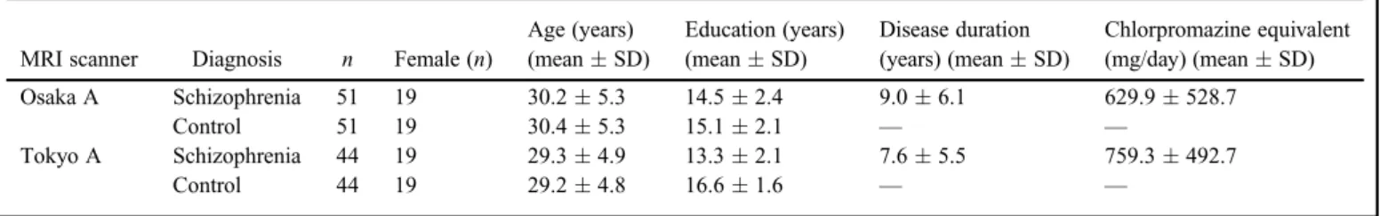
recruited from the University of Osaka and the University of Tokyo. We chose these two institutes because demographics of patients in these two institutes were similar and both had a sufficient number of healthy control subjects for balanced datasets. As the number of sub-jects scanned at the University of Osaka was greater than that at the University of Tokyo, we first selected a balanced dataset from the University of Tokyo, and then chose sex- and age-matched subjects from the University of Osaka. The remaining data from the University of Osaka were used for Dataset B, which is described in the following section. Each patient with schizophrenia was assessed and diagnosed according to the DSM-IV by at least two trained psychiatrists. Con-trols were recruited through local advertisements and evaluated via the DSM-IV Structured Clinical Interview, Non-Patient Version.22 Subjects were excluded if they had neurological or medical conditions that could potentially affect the central nervous system, such as atypi-cal headache, head trauma with loss of consciousness, chronic lung disease, kidney disease, chronic hepatic disease, thyroid disease, active stage cancer, cerebrovascular disease, and epilepsy or seizures. Subject demographics are summarized in Table 1. The total pre-scribed antipsychotics being taken by patients was calculated using chlorpromazine equivalent (mg/day) based on Inada and Inagaki.23
Subjects to evaluate the model (Dataset B)
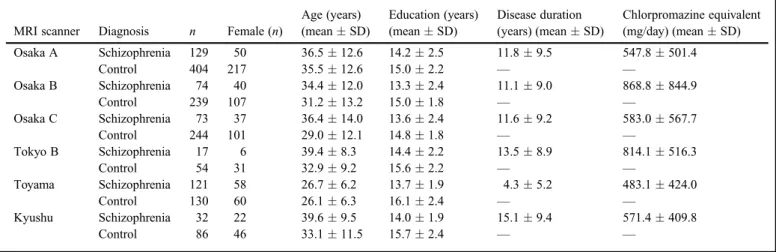
For the evaluation of the model we propose in this study, we used a total sample of 1603 subjects (schizophrenia: 446; control: 1157) from Osaka University, University of Tokyo, University of Toyama, and Kyushu University. The subjects in this dataset were independent of the subjects in Dataset A. As we wanted to estimate how useful our model would be in clinical settings, we did not match age and sex between patients and control subjects. Subject demographics are sum-marized in Table 2. This study was approved by the ethics commit-tees of each institute and performed in accordance with the guidelines and regulations of these research institutions. All participants gave written informed consent prior to participation.
MRI data acquisition
MRI data were obtained using seven different scanners. A 3-D volu-metric acquisition of a T1-weighted sequence produced a gapless series of sagittal sections. Table 3 provides a summary of the MRI scanners and the pulse sequences for each scanner.
Preprocessing of imaging
All of the MR images were processed usingSPM12 (Wellcome
Depart-ment of Imaging Neuroscience, University College London, UK, http:// www.fil.ion.ucl.ac.uk/spm) running on MATLAB R2015b (MathWorks,
Natick, MA, USA) on Ubuntu 16.04 based Lin4Neuro.24 Prior to
preprocessing, all data were co-registered to‘icbm152’standard image implemented inSPM12 so that the origin of images would be close to the
anterior commissure–posterior commissure (AC-PC) and so that images would be aligned with the AC-PC line. Each image was segmented into gray matter (GM), white matter (WM), and cerebrospinalfluid (CSF) using the segment function ofSPM12. Subsequently, the segmented GM
images were spatially normalized using diffeomorphic anatomical regis-tration through an exponentiated lie algebra (DARTEL) algorithm.25
Custom DARTEL templates were generated from all the GM and WM
Table 1. Demographics of Dataset A subjects MRI scanner Diagnosis n Female (n)
Age (years) (meanSD) Education (years) (meanSD) Disease duration (years) (meanSD) Chlorpromazine equivalent (mg/day) (meanSD) Osaka A Schizophrenia 51 19 30.25.3 14.52.4 9.06.1 629.9528.7 Control 51 19 30.45.3 15.12.1 — — Tokyo A Schizophrenia 44 19 29.34.9 13.32.1 7.65.5 759.3492.7 Control 44 19 29.24.8 16.61.6 — —
Psychiatry and Clinical Neurosciences 74: 56–63, 2020 57
PCN
Psychiatry andimages of the participants. After spatial normalization, the GM images were modulated to preserve the volume, followed by smoothing with an 8-mm full width at half maximum Gaussian kernel. For this preprocessing, default parameters were used. In addition to that, total intracranial volume (TIV) was calculated by summing GM image, WM image, and CSF image using the‘Tissue Volumes’function ofSPM12.
ROI for schizophrenia
We used the ‘two-sample t-test’ model implemented in SPM12 to
detect regions where patients with schizophrenia exhibited decreased volume compared with control subjects. Age, sex, and TIV were input as covariates of no interest. In addition, to consider the use of two different MRI scanners, we added another column to the design matrix to account for scanner difference and designated‘one’for one scanner and‘zero’for the second scanner as done by Mechelliet al. for multi-scanner data analysis.26As we wanted to obtain robust ROI, we employed conservative statistical thresholds for both peak-level and cluster-level. As for peak-level, statistical threshold was set to a family-wise error (FWE)-corrected P-value of <0.05. With this threshold as a cluster-defining threshold, an extent threshold of
250 voxels, which corresponded to a false discovery rate (FDR)-correctedP-value of <0.05, was set as a cluster-level threshold. We should note that we employed FDR instead of FWE for cluster-level correction because the FWE-correctedP-value of <0.05 corresponded to only one voxel. As described in the Results section, the ROI com-prised four clusters. Since voxel values within these clusters were highly correlated with each other, handling the values of each cluster separately would introduce a multicollinearity problem. Therefore, we united the clusters to form one ROI, binarized it, and obtained the averaged modulated volume within the united ROI as a single value for each subject.
Feature definition and statistical analysis
In clinical settings, MRI parameters vary from site to site. In this situ-ation, it is almost impossible to accommodate a wide variety of scan-ner differences with a single model. Therefore, we employed a strategy to determine the coefficients of a model for each MRI scan-ner. Voxel values of MRI data are subject to MRI scanner differences as well as various subject factors, such as age, sex, TIV, or disease. In order to estimate the effect of MRI scanners accurately, we also
Table 2. Demographics of Dataset B subjects MRI scanner Diagnosis n Female (n)
Age (years) (meanSD) Education (years) (meanSD) Disease duration (years) (meanSD) Chlorpromazine equivalent (mg/day) (meanSD) Osaka A Schizophrenia 129 50 36.512.6 14.22.5 11.89.5 547.8501.4 Control 404 217 35.512.6 15.02.2 — — Osaka B Schizophrenia 74 40 34.412.0 13.32.4 11.19.0 868.8844.9 Control 239 107 31.213.2 15.01.8 — — Osaka C Schizophrenia 73 37 36.414.0 13.62.4 11.69.2 583.0567.7 Control 244 101 29.012.1 14.81.8 — — Tokyo B Schizophrenia 17 6 39.48.3 14.42.2 13.58.9 814.1516.3 Control 54 31 32.99.2 15.62.2 — — Toyama Schizophrenia 121 58 26.76.2 13.71.9 4.35.2 483.1424.0 Control 130 60 26.16.3 16.12.4 — — Kyushu Schizophrenia 32 22 39.69.5 14.01.9 15.19.4 571.4409.8 Control 86 46 33.111.5 15.72.4 — —
Table 3. Summary of MRI scanners and pulse sequences
Osaka A Osaka B Osaka C Tokyo A Tokyo B Toyama Kyushu
Manufacturer GE GE GE GE GE Siemens Philips
Scanner name Signa EXCITE Signa Hdxt Discovery MR750
Signa Horizon Discovery MR750w
Magnetom Vision
Achieva
Magnet strength 1.5 T 3 T 3 T 1.5 T 3 T 1.5 T 3 T
Head coil Head QD 8HRBRAIN HNS Head Circularly
polarized head
Head 24 CP head 8ch head
Pulse sequence Fast SPGR Fast SPGR Fast SPGR SPGR SPGR FLASH 3D T1-TFE
Number of slices 124 172 156 124 200 160 190
Echo time (ms) 4.2 2.9 3.2 7 3.1 10 3.8
Repetition time (ms) 12.6 7.2 8.2 35 7.7 24 8.2
Flip angle (degree) 15 11 11 30 11 40 8
Acquisition matrix 256×256 256×256 256×256 256×256 256×256 256×256 240×240 Number of excitations (NEX) 1 1 1 1 1 1 1 Field of view (cm) 24×24 24×24 26×26 24×24 26×26 25.6×25.6 24×24 Voxel dimension (mm) 0.9×0.9×1.4 0.9×0.9×1.0 1.0×1.0×1.2 0.9×0.9×1.5 1.0×1.0×1.2 1.0×1.0×1.0 1.0×1.0×1.0 Slice thickness (mm) 1.4 1.0 1.2 1.5 1.2 1.0 1.0
considered age, sex, and TIV in the model and estimated the effect of MRI scanners using healthy control MRI data. This process is similar to preparing a standard for a control experiment. We chose a general-linear-model-based approach to extract a feature for differentiation. Though recent studies have tended to employ a machine-learning approach or multivariate analysis to extract features for classification, it is difficult to evaluate the effect of how MRI scanner differences are considered with these approaches. Therefore, we used a simple linear model to see if the model could minimize scanner differences. Using modulated volume within ROI as an objective variable (Y), we defined the model as follows:
Y =
β
1×
Age +
β
2×
Sex +
β
3×
TIV +
C
+
ε
,
where the betas are coefficients for each independent variable,Cis a constant term in which we expect to include the scanner factor, andε is the residual, which we use as a classification feature. Given a design matrix Y consisting of modulated volumes within the ROI (n×1 matrix where n is the number of subjects), X consisting of age, sex, TIV and‘one’for each subject (n×4 matrix), B consisting of β1, β2, β3, and C (4×1 matrix), and E consisting of residuals
(n×1 matrix), the formula can also be described as follows:
Y = XB + E
According to the ordinary least square method, B is estimated by multiplying the inversion matrix of X by Y. However, X is not a square matrix here, so we cannot directly compute the inversion matrix of X. In this situation, considering XT, which is the transposed matrix of X, XTX will always be a square matrix, so using the inver-sion matrix of XTX, (XTX)−1, B can be estimated.
Y = XB
X
TY = X
TXB
X
TX
−1X
TY = X
TX
−1X
TXB
X
TX
−1X
TY = B
This computation can be easily done withMATLABusing thepinv function (B = pinv(X)*Y), so we usedMATLABR2015b to estimate the Matrix B. After obtaining B, we applied Formula 1 to all subjects for each scanner to obtain Matrix E, which comprisesεfor each subject. Matrix E represents the ‘schizophrenia likeness’ feature by
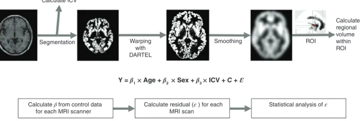
minimizing the MRI scanner effect and adjusting for age, sex, and TIV at the same time. Figure 1 is the processingflowchart. We then performed receiver–operator curve (ROC) analysis with the ROCR package in R 3.4.3 (R Foundation for Statistical Computing, Vienna, Austria) to evaluate the accuracy of the differentiation.27
Validation of our method
Our method for deciding the coefficient of the model is entirely dependent on control subjects. We explored how coefficients from different datasets would affect the results of ROC analysis. As Osaka A was the largest dataset in Dataset B, we used it for validation. We randomly divided the Osaka A dataset into two subsets. We prepared Matrices Y1and X1from Subset 1 and Matrices Y2and X2from
Sub-set 2. From the control subjects of SubSub-set 1, we calculated coefficient Matrix B1. We also calculated coefficient Matrix B2from the control
subjects of Subset 2. Then we calculated the residual Matrix E1from
Subset 1 with E1= Y1–X1B2and the residual Matrix E2from Subset
2 with E2 = Y2 – X2B1. ROC analyses were performed on these
residuals.
Results
ROI for schizophrenia
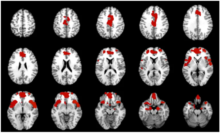
Figure 2 and Table 4 show the ROI we used for further analysis. Patients with schizophrenia showed a significant gray matter volume reduction in the bilateral insulae, superior temporal gyri, the middle frontal gyri, the medial portion of the superior frontal gyri, and the hippocampi. These results are consistent with a previous meta-analysis,5–7so we used these areas as our ROI. We did notfind any volume increase in patients with schizophrenia with the statistical threshold we employed.
ROC analysis
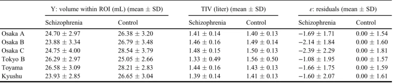
Table 5 shows the statistics for Dataset B. Figure 3 and Table 6 show the results of ROC analysis. The purpose of this study was to evaluate how a single model with a certain feature can be applied to different sites, so we adopted a single cut-off among analyses. ROC analysis with the Osaka A scanner (GE 1.5T) with the largest sample in this study revealed that the cut-off score of the closest point to (0, 1) in the ROC curve was−1.3. Therefore, we applied this value (−1.3) as a cut-off score to evaluate sensitivity, specificity, and accuracy for each ROC analysis. As a result, sensitivity ranged from 47% to 67% as well as specificity from 75% to 84%. The area under the curve (AUC) ranged from 0.74 to 0.84 and accuracy ranged from 69% to 76%. ROC analysis with all samples revealed an AUC of 0.76 and an
Calculate ICV Segmentation Warping with DARTEL Smoothing ROI Calculate regional volume within ROI
Y = β1 ×Age + β2× Sex + β3 × ICV + C + Ɛ
Calculate β from control data for each MRI scanner
Calculate residual (ε ) for each MRI scan
Statistical analysis of ε
Fig.1Scheme of feature extraction. Segmentation of 3-D T1-weighted image was performed to extract gray matter image and intracranial volume (ICV), followed by anatomical normalization with diffeomorphic anatomical registration through an exponentiated lie algebra (DARTEL) and smoothing. Then the within-region-of-interest (ROI) volume was calculated. Using this volume as a dependent variable Y, a general linear model wasfitted considering age, sex, ICV, and a constant that could reflect scanner differences for each MRI scanner. Then the residualεfor each subject was calculated and this value was treated as a differentiation feature.
Psychiatry and Clinical Neurosciences 74: 56–63, 2020 59
PCN
Psychiatry andaccuracy of 73%. Table S1 shows the ROC results for the two subsets of Osaka A. The results were similar, which indicates the validity of our method to some extent.
Discussion
In this study, we tried to minimize the effect of scanner differences for differentiation of schizophrenia patients from control subjects.
Even with a single cut-off score, overall accuracy remained around 70% among different sites/scanners, which implies the reproducibility of our model for different datasets. Our results also have the potential-ity for clinical application. Conventionally, in order tofind the schizo-phrenia likeness from brain MRI data, one needs to prepare datasets for large numbers of patients and controls. In this situation, if a facility’s MRI scanner is replaced, researchers and physicians must create entirely new datasets with data from the new machine.
Fig.2Regions of interest (ROI) for this study. ROI are defined from group comparisons between 95 patients with schizophrenia and age- and sex-matched controls. Statistical threshold was set to a family-wise-error-correctedP-value of <0.01 with an extent threshold of 100 voxels. These regions include the bilateral superior tem-poral gyri, the middle frontal gyri, the medial portion of the superior frontal gyri, and hippocampi.
Table 4. Volume reduction in patients with schizophrenia using Dataset A
Cluster Region Cluster size
Cluster-level FDR corrected P Peak-level FWE corrected P T MNI coordinates x y z
Cluster 1 Lt. anterior insula 4787 <0.001 <0.001 8.34 −36 23 −5
Lt. hippocampus <0.001 6.58 −14 −6 −15
Lt. opercular part of inferior frontal gyrus <0.001 6.12 −50 12 4
Cluster 2 Rt. anterior insula 2792 <0.001 <0.001 7.48 39 21 −3
Rt. planum polare <0.001 7.03 57 −1 1
Rt. posterior orbital gyrus <0.001 6.9 36 18 −18
Cluster 3 Rt. medial frontal gyrus 5489 <0.001 <0.001 7.46 2 41 −20
Lt. superior frontal lobe medial segment <0.001 7.06 −3 51 3
Lt. medial frontal gyrus <0.001 6.93 0 54 −11
Cluster 4 Lt. middle cingulate gyrus 810 <0.001 <0.001 6.38 −8 −13 39
Rt. middle cingulate gyrus 0.003 5.38 6 −25 36
However, the model we propose in this study requires only control subjects for a specific MRI scanner. Once the coefficients of the model are determined, we can apply the model to as few as one patient, eliminating the need for multiple datasets from multiple
individuals, to see if that single patient has a schizophrenia likeness.
Though there are various reports that have discussed the classifi -cation of schizophrenia patients from a control group using structural
Table 5. Statistics of Dataset B
Y: volume within ROI (mL) (meanSD) TIV (liter) (meanSD) ε: residuals (meanSD)
Schizophrenia Control Schizophrenia Control Schizophrenia Control
Osaka A 24.702.97 26.383.20 1.410.14 1.400.13 −1.691.71 0.001.54 Osaka B 23.883.34 26.793.48 1.460.16 1.490.14 −2.141.84 0.001.60 Osaka C 24.754.00 28.543.79 1.480.15 1.500.13 −2.392.29 0.001.81 Tokyo B 26.292.97 25.052.66 1.330.49 1.560.50 −1.081.95 0.001.57 Toyama 26.583.09 28.212.83 1.440.16 1.430.13 −1.661.75 0.001.59 Kyushu 23.932.85 26.653.04 1.390.14 1.410.13 −1.602.07 0.001.61
ROI, region of interest; TIV, total intracranial volume.
0 0 0.2 0.4 0.6 0.8 1 0.2 0.4 False Positive Rate
True Positive Rate
0.6 Osaka A
Tokyo B Toyama Kyushu All
Osaka B Osaka C 0.8 1 0 0 0.2 0.4 0.6 0.8 1 0.2 0.4 0.6 0.8 1 0 0 0.2 0.4 0.6 0.8 1 0.2 0.4 0.6 0.8 1 0 0 0.2 0.4 0.6 0.8 1 0.2 0.4 0.6 0.8 1 0 0 0.2 0.4 0.6 0.8 1 0.2 0.4 0.6 0.8 1 0 0 0.2 0.4 0.6 0.8 1 0.2 0.4 0.6 0.8 1 0 0 0.2 0.4 0.6 0.8 1 0.2 0.4 0.6 0.8 1 Fig.3Receiver–operator curve (ROC) analysis. The area under the curve (AUC) ranged from 0.74 to 0.84, and accuracy from 69% to 76%. ROC analysis with all sam-ples revealed an AUC of 0.76 and an accuracy of 73%.
Table 6. Results of receiver–operator curve analysis
Osaka A Osaka B Osaka C Tokyo B Toyama Kyushu All data
Schizophrenia 129 74 73 17 121 32 446
Control 404 239 244 54 130 86 1157
Area under curve 0.78 0.84 0.83 0.68 0.76 0.74 0.76
Sensitivity 0.60 0.67 0.70 0.44 0.57 0.56 0.63
Specificity 0.81 0.80 0.77 0.84 0.79 0.80 0.75
Positive predictive value 0.49 0.50 0.47 0.47 0.71 0.51 0.34
Negative predictive value 0.86 0.88 0.89 0.82 0.66 0.83 0.91
Accuracy 0.76 0.76 0.74 0.74 0.69 0.74 0.73
Psychiatry and Clinical Neurosciences 74: 56–63, 2020 61
PCN
Psychiatry andMRI, multisite studies are limited. Rozycki and colleagues used mul-tivariate analysis tools and found a neuroanatomical signature of patients with schizophrenia, with which they achieved a prediction accuracy of 72%–77%.28 They took into account the effect of MRI scanner as a variable in the multivariate analysis. Our results are simi-lar to theirs, which substantiates that structural MRI could be a useful tool for schizophrenia at the individual level and indicates that our approach of considering the MRI scanner as a factor in the model could be as effective as their approach. From a diagnostic point of view, the accuracy of our method did not exceed the previous reports. Meta-analysis of brain volumes in schizophrenia showed that effect sizes for gray matter structures ranged from −0.22 to −0.58.29This effect size means that there is substantial overlap between patients with schizophrenia and controls. In this context, it might be difficult to improve the accuracy of classification with structural data alone. Another point of our result is that specificity is generally higher than sensitivity in each site of Dataset B. Florkowski indicates that high sensitivity is the ideal property of a‘rule-out’test while high specifi c-ity is the ideal property of a ‘rule-in’ test.30 Considering this, our results suggest that our method might be suitable to rule-in the possi-bilities of schizophrenia rather than rule-out.
Not only structural MRI, but also other modalities, such as func-tional MRI (fMRI) or diffusion tensor imaging, could contribute to the differentiation of schizophrenia at the individual level. Recent studies using the Alzheimer’s Disease Neuroimaging Initiative dataset to investigate the combined biomarkers from different modalities, such as structural MRI, fMRI,fluorodeoxyglucose–positron emission tomography, or CSF, to discriminate between Alzheimer’s disease, mild cognitive impairment, and control reported that classification accuracy with a combination of modalities was better than that with a single modality.31–33Similar results have been reported for the
classi-fication of schizophrenia. Yang et al. reported that a classifier of schizophrenia using combined features of structural and functional MRI data achieved higher accuracy than did a single-modal-features method.34 However, no multisite studies on the differentiation of schizophrenia using multimodal imaging have been reported to date. Scanner differences need to be considered for diffusion tensor imag-ing or fMRI as well as for structural MRI. Our approach might pro-vide a means to identify appropriate features of different modalities while also considering scanner differences.
There are several limitations in our study. Our method for decid-ing the coefficient of the model was entirely dependent on control subjects. Though we showed that coefficients from different control subjects did not change the result much, we have not explored the minimum number of subjects required in order to obtain robust results. In Dataset B, Tokyo B and Kyushu resulted in low sensitivi-ties. The sample sizes of the control group for the Tokyo B and Kyu-shu datasets were relatively small (less than 100) compared with those for other facilities, which might have affected the results. We must also consider the variation in control subjects. In Dataset B, the subjects for Toyama were young and the standard deviation of age was small. In this situation, two things need to be considered: (i) brain volume changes might be subtle due to the shorter duration of disease; and (ii) overfitting might occur when calculating coeffi -cients, as the range of variables is limited. We used as many control subjects as possible for this study, but in order for this approach to become feasible in a clinical setting, further study is necessary to determine the minimal sample size for control subjects. At the same time, the Alzheimer’s Disease Neuroimaging Initiative uses phantom and common pulse sequence to obtain images of similar quality across MRI scanners. This kind of approach might also be useful in our model. Another limitation is that the ROI we employed was deter-mined using only 1.5-T MRI scanners. Though we set a statistically conservative threshold in order to generate a robust ROI and the results were consistent with a previous meta-analysis,5–7 larger bal-anced datasets using different MRI scanners might be necessary to generate a more robust ROI. One other limitation is that most of the subjects with schizophrenia were on medication. It is known that
antipsychotics can affect brain volume, especially subcortical vol-ume.35As our model depends upon control subjects, we did not take the medication dose into account. However, we defined the ROI with a conservative threshold (family wise error P< 0.05 with extent threshold of 250 voxels) in order to ensure the use of robust regions for the present analysis.
In conclusion, we demonstrated that in considering scanner dif-ferences we could differentiate schizophrenia from control using structural MRI across multiple sites. This could be a useful method for applying neuroimaging techniques to a clinical setting in order to achieve an accurate diagnosis of schizophrenia.
Acknowledgments
This work was supported by the Brain Mapping by Integrated Neurotechnologies for Disease Studies (Brain/MINDS; Grant Num-ber: JP18dm0207006 to RH), Brain/MINDS Beyond (Grant NumNum-ber: JP18dm0307002 to RH), Japan Agency for Medical Research and Development (AMED; Grant Number 16dk0307031h0003 to K.N., T.O., M.S., K.K., and R.H.), and the Grants-in-Aid for Scientific Research (KAKENHI; Grant Number JP25293250 and JP16H05375 to R.H., and JP18K18164 to K.N.).
Disclosure statement
The authors declare no conflicts of interest.
Author contributions
K.N. was critically involved in analysis and wrote thefirst draft of the manuscript. T.S., M.F., F.Y., and M.T. were involved in the data analysis and contributed to the interpretation of the data. H.Y., Y.Y., H.A., N.K., Y.W., M.K., T.T., S.K., N.O., Y.H., T.O., H.Y., M.S., and K.K. were involved in data collection and contributed to the inter-pretation of the data. T.A. was involved in the interinter-pretation of the data and critical review of the manuscript. R.H. supervised the entire project, collected the data, and was critically involved in the design and interpretation of the data. All authors contributed to and approved thefinal manuscript.
References
1. American Psychiatric Association.Diagnostic and Statistical Manual of Mental Disorders, 5th edn. American Psychiatric Association Publishing, Washington, DC, 2013.
2. Rössler W, Joachim Salize H, van Os J, Riecher-Rössler A. Size of bur-den of schizophrenia and psychotic disorders. Eur. Neuro-psychopharmacol.2005;15: 399–409.
3. Shenton ME, Dickey CC, Frumin M, McCarley RW. A review of MRI
findings in schizophrenia.Schizophr. Res.2001;49: 1–52.
4. Honea R, Sc B, Crow TJet al. Regional deficits in brain volume in schizophrenia: A meta-analysis of voxel-based morphometry studies.
Am. J. Psychiatry2005;162: 2233–2245.
5. Glahn DC, Laird AR, Ellison-Wright Iet al. Meta-analysis of gray mat-ter anomalies in schizophrenia: Application of anatomic likelihood esti-mation and network analysis.Biol. Psychiatry2008;64: 774–781. 6. Fornito A, Yücel M, Patti J, Wood SJ, Pantelis C. Mapping grey matter
reductions in schizophrenia: An anatomical likelihood estimation analy-sis of voxel-based morphometry studies. Schizophr. Res. 2009; 108: 104–113.
7. Bora E, Fornito A, Radua J et al. Neuroanatomical abnormalities in schizophrenia: A multimodal voxelwise analysis and meta-regression analysis.Schizophr. Res.2011;127: 46–57.
8. Takahashi T, Suzuki M. Brain morphologic changes in early stages of psychosis: Implications for clinical application and early intervention.
Psychiatry Clin. Neurosci.2018;72: 556–571.
9. van Erp TGM, Hibar DP, Rasmussen JMet al. Subcortical brain volume abnormalities in 2028 individuals with schizophrenia and 2540 healthy con-trols via the ENIGMA Consortium.Mol. Psychiatry2016;21: 547–553. 10. Okada N, Fukunaga M, Yamashita Fet al. Abnormal asymmetries in
subcortical brain volume in schizophrenia. Mol. Psychiatry 2016; 21: 1460–1466.
11. Leonard CM, Kuldau JM, Breier JIet al. Cumulative effect of anatomi-cal risk factors for schizophrenia: An MRI study.Biol. Psychiatry1999;
12. Csernansky JG, Schindler MK, Splinter NRet al. Abnormalities of tha-lamic volume and shape in schizophrenia.Am. J. Psychiatry2004;161: 896–902.
13. Nakamura K, Kawasaki Y, Suzuki M et al. Multiple structural brain measures obtained by three-dimensional magnetic resonance imaging to distinguish between schizophrenia patients and normal subjects.
Schizophr. Bull.2004;30: 393–404.
14. Davatzikos C, Shen D, Gur RCRE et al. Whole-brain morphometric study of schizophrenia revealing a spatially complex set of focal abnor-malities.Arch. Gen. Psychiatry2005;62: 1218–1227.
15. Kawasaki Y, Suzuki M, Kherif Fet al. Multivariate voxel-based mor-phometry successfully differentiates schizophrenia patients from healthy controls.NeuroImage2007;34: 235–242.
16. Yoon U, Lee J-M, Im Ket al. Pattern classification using principal com-ponents of cortical thickness and its discriminative pattern in schizophre-nia.NeuroImage2007;34: 1405–1415.
17. Pohl KM, Sabuncu MR. A unified framework for MR based disease clas-sification.Inf. Process. Med. Imaging2009;21: 300–313.
18. Ota M, Sato N, Ishikawa Met al. Discrimination of female schizophrenia patients from healthy women using multiple structural brain measures obtained with voxel-based morphometry. Psychiatry Clin. Neurosci.
2012;66: 611–617.
19. Zanetti MV, Schaufelberger MS, Doshi Jet al. Neuroanatomical pattern classification in a population-based sample offirst-episode schizophrenia.
Prog. Neuropsychopharmacol. Biol. Psychiatry2013;43: 116–125. 20. Kambeitz J, Kambeitz-Ilankovic L, Leucht Set al. Detecting
neuroimag-ing biomarkers for schizophrenia: A meta-analysis of multivariate pattern recognition studies.Neuropsychopharmacology2015;40: 1742–1751. 21. Kruggel F, Turner J, Muftuler LT, Alzheimer’s Disease Neuroimaging
Initiative. Impact of scanner hardware and imaging protocol on image quality and compartment volume precision in the ADNI cohort.
NeuroImage2010;49: 2123–2133.
22. Shear MK, Greeno C, Kang Jet al. Diagnosis of nonpsychotic patients in community clinics.Am. J. Psychiatry2000;157: 581–587.
23. Inada T, Inagaki A. Psychotropic dose equivalence in Japan.Psychiatry Clin. Neurosci.2015;69: 440–447.
24. Nemoto K, Dan I, Rorden Cet al. Lin4Neuro: A customized Linux distri-bution ready for neuroimaging analysis.BMC Med. Imaging2011;11: 3.
25. Ashburner J. A fast diffeomorphic image registration algorithm.
NeuroImage2007;38: 95–113.
26. Mechelli A, Riecher-Rössler A, Meisenzahl EMet al. Neuroanatomical abnormalities that predate the onset of psychosis: A multicenter study.
Arch. Gen. Psychiatry2011;68: 489–495.
27. Sing T, Sander O, Beerenwinkel N, Lengauer T. ROCR: Visualizing classifier performance in R.Bioinformatics2005;21: 3940–3941. 28. Rozycki M, Satterthwaite TD, Koutsouleris Net al. Multisite machine
learning analysis provides a robust structural imaging signature of schizophrenia detectable across diverse patient populations and within individuals.Schizophr. Bull.2018;44: 1035–1044.
29. Haijma SV, Van Haren N, Cahn W, Koolschijn PCMP, Hulshoff Pol HE, Kahn RS. Brain volumes in schizophrenia: A meta-analysis in over 18 000 subjects.Schizophr. Bull.2013;39: 1129–1138.
30. Florkowski CM. Sensitivity, specificity, receiver-operating characteristic (ROC) curves and likelihood ratios: Communicating the performance of diagnostic tests.Clin. Biochem. Rev.2008;29: S83–S87.
31. Gray KR, Aljabar P, Heckemann RA, Hammers A, Rueckert D. Random forest-based similarity measures for multi-modal classification of Alzheimer’s disease.NeuroImage2013;65: 167–175.
32. Zhang Z, Huang H, Shen D, Alzheimer’s Disease Neuroimaging Initia-tive. Integrative analysis of multi-dimensional imaging genomics data for Alzheimer’s disease prediction.Front. Aging Neurosci.2014;6: 260. 33. Zhang D, Wang Y, Zhou L, Yuan H, Shen D, Alzheimer’s Disease
Neu-roimaging Initiative. Multimodal classification of Alzheimer’s disease and mild cognitive impairment.NeuroImage2011;55: 856–867. 34. Yang H, He H, Zhong J. Multimodal MRI characterisation of
schizo-phrenia: A discriminative analysis.Lancet2016;388: S36.
35. Hashimoto N, Ito YM, Okada Net al. The effect of duration of illness and antipsychotics on subcortical volumes in schizophrenia: Analysis of 778 subjects.NeuroImage Clin.2018;17: 563–569.
Supporting information
Additional Supporting Information may be found in the online ver-sion of this article at the publisher’s web-site:
Table S1.Results of ROC analysis on Osaka A subset data.
Psychiatry and Clinical Neurosciences 74: 56–63, 2020 63
PCN
Psychiatry and