Introduction to the Maxwell Garnett approximation:
tutorial
Vadim Markel
To cite this version:
Vadim Markel. Introduction to the Maxwell Garnett approximation: tutorial . Journal of
the Optical Society of America A, Optical Society of America, 2016, 33 (7), pp.1244-1256.
<
10.1364/JOSAA.33.001244
>
.
<
hal-01282105v2
>
HAL Id: hal-01282105
https://hal.archives-ouvertes.fr/hal-01282105v2
Submitted on 3 Jun 2016
HAL
is a multi-disciplinary open access
archive for the deposit and dissemination of
sci-entific research documents, whether they are
pub-lished or not.
The documents may come from
teaching and research institutions in France or
abroad, or from public or private research centers.
L’archive ouverte pluridisciplinaire
HAL
, est
destin´
ee au d´
epˆ
ot et `
a la diffusion de documents
scientifiques de niveau recherche, publi´
es ou non,
´
emanant des ´
etablissements d’enseignement et de
recherche fran¸cais ou ´
etrangers, des laboratoires
publics ou priv´
es.
Introduction to Maxwell Garnett approximation: tutorial
VADIM
A. MARKEL
∗Aix-Marseille Université, CNRS, Centrale Marseille, Institut Fresnel UMR 7249, 13013 Marseille, France [email protected]
Compiled May 2, 2016
This tutorial is devoted to the Maxwell Garnett approximation and related theories. Topics covered in this first, introductory part of the tutorial include the Lorentz local field correction, the Clausius-Mossotti rela-tion and its role in the modern numerical technique known as the Discrete Dipole Approximarela-tion (DDA), the Maxwell Garnett mixing formula for isotropic and anisotropic media, multi-component mixtures and the Bruggeman equation, the concept of smooth field, and Wiener and Bergman-Milton bounds. © 2016 Optical Society of America
OCIS codes: (000.1600) Classical and quantum physics; (160.0160) Materials.
http://dx.doi.org/10.1364/JOSAA.XX.XXXXXX
1. INTRODUCTION
In 1904, Maxwell Garnett [1] has developed a simple but im-mensely successfulhomogenization theory. As any such theory, it aims to approximate a complex electromagnetic medium such as a colloidal solution of gold micro-particles in water with a homogeneouseffective medium. The Maxwell Garnettmixing for-mulagives the permittivity of this effective medium (or, sim-ply, the effective permittivity) in terms of the permittivities and volume fractions of the individual constituents of the complex medium.
A closely related development is the Lorentz molecular the-ory of polarization. This thethe-ory considers a seemingly different physical system: a collection of point-like polarizable atoms or molecules in vacuum. The goal is, however, the same: compute the macroscopic dielectric permittivity of the medium made up by this collection of molecules. A key theoretical ingredient of the Lorentz theory is the so-called local field correction, and this ingredient is also used in the Maxwell Garnett theory.
The two theories mentioned above seem to start from very different first principles. The Maxwell Garnett theory starts from the macroscopic Maxwell’s equations, which are assumed to be valid on a fine scale inside the composite. The Lorentz the-ory does not assume that the macroscopic Maxwell’s equations are valid locally. The molecules can not be characterized by macroscopic quantities such as permittivity, contrary to small inclusions in a composite. However, the Lorentz theory is still macroscopic in nature. It simply replaces the description of inclusions in terms of the internal field and polarization by a cumulative characteristic called the polarizability. Within the approximations used by both theories, the two approaches are
∗On leave from the Department of Radiology, University of Pennsylvania,
Philadelphia, Pennsylvania 19104, USA; [email protected]
mathematically equivalent.
An important point is that we should not confuse the the-ories ofhomogenization that operate with purely classical and macroscopic quantities with the theories that derive the macro-scopic Maxwell’s equations (and the relevant constitutive pa-rameters) from microscopic first principles, which are in this case the microscopic Maxwell’s equations and the quantum-mechanical laws of motion. Both the Maxwell Garnett and the Lorentz theories are of the first kind. An example of the sec-ond kind is the modern theory of polarization [2,3], which com-putes the induced microscopic currents in a condensed medium (this quantity turns out to be fundamental) by using the density-functional theory (DFT).
This tutorial will consist of two parts. In the first, introduc-tory part, we will discuss the Maxwell Garnett and Lorentz theories and the closely related Clausius-Mossotti relation from the same simple theoretical viewpoint. We will not attempt to give an accurate historical overview or to compile an exhaus-tive list of references. It would also be rather pointless to write down the widely known formulas and make several plots for model systems. Rather, we will discuss the fundamental un-derpinnings of these theories. In the second part, we will dis-cuss several advanced topics that are rarely covered in the text-books. We will then sketch a method for obtaining more general homogenization theories in which the Maxwell Garnett mixing formula serves as the zeroth-order approximation.
Over the past hundred years or so, the Maxwell Garnett ap-proximation and its generalizations have been derived by many authors using different methods. It is unrealistic to cover all these approaches and theories in this tutorial. Therefore, we will make an unfortunate compromise and not discuss some important topics. One notable omission is that we will not
dis-cuss random media [4–6] in any detail, although the first part of the tutorial will apply equally to both random and determin-istic (periodic) media. Another interesting development that we will not discuss is the so-called extended Maxwell Garnett theories [7–9] in which the inclusions are allowed to have both electric and magnetic dipole moments.
Gaussian system of units will be used throughout the tuto-rial.
2. LORENTZ LOCAL FIELD CORRECTION, CLAUSIUS-MOSSOTTI RELATION AND MAXWELL GARNETT MIXING FORMULA
The Maxwell Garnett mixing formula can be derived by differ-ent methods, some being more formal than the others. We will start by introducing the Lorentz local field correction and deriv-ing the Clausius-Mossotti relation. The Maxwell Garnett mix-ing formula will follow from these results quite naturally. We emphasize, however, that this is not how the theory has pro-gressed historically.
A. Average field of a dipole
The key mathematical observation that we will need is this: the integral over any finite sphere of the electric field created by a static point dipoledlocated at the sphere’s center is not zero but equal to−(4π/3)d.
The above statement may appear counterintuitive to anyone who has seen the formula for the electric field of a dipole,
Ed(r) = 3ˆ
r(rˆ·d)−d
r3 , (1)
where ˆr = r/r is the unit vector pointing in the direction of the radius-vectorr. Indeed, the angular average of the above expression is zero [10]. Nevertheless, the statement made above is correct. The reason is that the expression (1) is incomplete. We should have written
Ed(r) = 3ˆ
r(ˆr·d)−d
r3 −
4π
3 δ(r)d, (2) whereδ(r)is the three-dimensional Dirac delta-function.
The additional delta-term in (2) can be understood from many different points of view. Three explanations of varying degree of mathematical rigor are given below.
(i) A qualitative physical explanation can be obtained if we consider two point chargesq/βand−q/βseparated by the dis-tanceβhwhereβis a dimensionless parameter. This set-up is illustrated in Fig.1. Now letβtend to zero. The dipole moment of the system is independent ofβand has the magnituded=qh. The field created by these two charges at distances r ≫ βhis indeed given by (1) where the direction of the dipole is along the axis connecting the two charges. But this expression does not describe the field in the gap. It is easy to see that this field scales as−q/(β3h2)while the volume of the region where this
very strong field is supported scales as β3h3. The spatial inte-gral of the electric field is proportional to the product of these two factors,−qh=−d. Then 4π/3 is just a numerical factor.
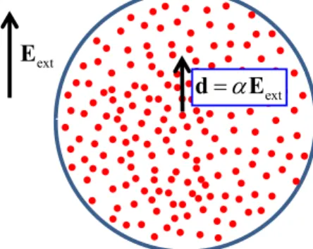
(ii) A more rigorous albeit not a very general proof can be obtained by considering a dielectric sphere of radiusaand per-mittivityǫin a constant external electric fieldEext. It is known
that the sphere will acquire a dipole momentd =αEextwhere
the static polarizabilityαis given by the formula
α=a3ǫ−1 ǫ+2. (3)
+
-q
-q
q
+
q
+
h
Z
q
!
"
q
! "# $
%
zE P
# !
q
h
P
zd
#
qh
Fig. 1.(color online) Illustration of the set-up used in the derivation (i) of the equation (2). The dipole moment of the system of two charges in theZ-direction isdz = qh. The
elec-tric field in the mid-pointPisEz(P) = −8q/β3h2. The oval
shows the region of space were the strong field is supported; its volume scales asβ3h3. Note that rigorous integration of the
electric field of a truly point charge is not possible due to a di-vergence. In this figure, the charges are shown to be of finite size. In this case, a small spherical region around each charge gives a zero contribution to the integral.
This result can be obtained by solving the Laplace equation with the appropriate boundary conditions at the sphere surface and at infinity. From this solution, we can find that the electric field outside of the sphere is given by (1) (plus the external field, of course) while the field inside is constant and given by
Eint= 3
ǫ+2Eext. (4)
The depolarizing field Edepis by definition the difference be-tween the internal field (the total field existing inside the sphere) and the external (applied) field. By the superposition principle,Eint=Eext+Edep. Thus,Edepis the field created by
the charge induced on the sphere surface. By using (4), we find that
−Edep=ǫ−1 ǫ+2Eext=
1
a3d. (5)
Integrating over the volume of the sphere, we obtain
Z
r<a
Edepd3r=−4π
3 d. (6) We can write more generally for anyR≥a,
Z r<R (E−Eext)d3r= Z r<R Edd3r=−4π 3 d. (7) The expression in the right-hand side of (7) is the pre-factor in front of the delta-function in (2).
(iii) The most general derivation of the singular term in (2) can be obtained by computing the static Green’s tensor for the electric field [11],
G(r,r′) =−∇r⊗ ∇r′ 1
|r−r′|. (8)
Here the symbol ⊗ denotes tensor product. For example,
(a⊗b)c=a(b·c),(a⊗b)αβ=aαbβ, etc. The singularity
origi-nates from the double differentiation of the non-analytical term
|r−r′|. This can be easily understood if we recall that, in one di-mension,∂2∂|xx∂−xx′′| =δ(x−x′). Evaluation of the right-hand side
+q -q +q -q -q +q -q-q -q -q +q -q -q -q -q -q -q !" !"
!
!
Fig. 2.(color online) A collection of dipoles in an external field. The particles are distributed inside a spherical volume either randomly (as shown) or periodically. It is assumed, however, that the macroscopic density of particles is constant inside the sphere and equal tov−1=N/V. Herevis the specific volume
per one particle.
of (8) is straightforward but lengthy, and we leave it for an ex-ercise. If we perform the differentiation accurately and then set
r′ =0, we will find thatG(r, 0)dis identical to the right-hand side of (2).
Now, the key approximation of the Lorentz molecular theory of polarization, as well as that of the Maxwell Garnett theory of composites, is that the regular part in the right-hand side of (2) averages to zero and, therefore, it can be ignored, whereas the singular part does not average to zero and should be retained. We will now proceed with applying this idea to a physical prob-lem.
B. Lorentz local field correction
Consider some spatial regionVof volumeVcontainingN≫1
small particles of polarizabilityαeach. We can refer to the par-ticles as to “molecules”. The only important physical property of a molecule is that it has a linear polarizability. The specific volume per one molecule isv=V/N. We will further assume thatVis connected and sufficiently “simple”. For example, we
can consider a plane-parallel layer or a sphere. In these two cases, the macroscopic electric field inside the medium is con-stant, which is important for the arguments presented below. The system under consideration is schematically illustrated in Fig.2.
Let us now place the whole system in a constant external electric fieldEext. We will neglect the electromagnetic
interac-tion of all the dipoles since we have decided to neglect the regu-lar part of the dipole field in (2). Again, the assumption that we use is that this field is unimportant because it averages to zero when summed over all dipoles. In this case, each dipole “feels” the external fieldEextand therefore it acquires the dipole mo-mentd=αEext. The total dipole moment of the object is
dtot=Nd=NαEext. (9)
On the other hand, if we assign the sample some macroscopic permittivityǫand polarizationP= [(ǫ−1)/4π]E, then the to-tal dipole moment is given by
dtot=VP=Vǫ−1
4π E. (10)
In the above expression,Eis the macroscopic electric field in-side the medium, which is, of course, different from the applied
fieldEext. To find the relation between the two fields, we can
use the superposition principle and write
E=Eext+ *
∑
n En(r) + , r∈V. (11)Here En(r) is the field produced by then-th dipole andh. . .i
denotes averaging over the volume of the sample. Of course, the individual fields En(r)will fluctuate and so will the sum
of all these contributions,∑nEn(r). The averaging in the
right-hand side of (11) has been introduced since we believe that the macroscopic electric field is a suitably defined average of the fast-fluctuating “microscopic” field.
We now compute the averages in (11) as follows:
hEn(r)i= 1 V Z VEd(r−rn)d 3r≈ −4π 3 d V , (12)
wherern is the location of then-th dipole andEd(r)is given
by (2). In performing the integration, we have disregarded the regular part of the dipole field and, therefore, the second equal-ity above is approximate. We now substitute (12) into (11) and obtain the following result:
E=Eext+
∑
n h Eni=Eext−N4π 3 d V = 1−4π 3 α v Eext. (13)In the above chain of equalities, we have usedd = αEextand V/N=v.
All that is left to do now is substitute (13) into (10) and use the condition that (9) and (10) must yield the same total dipole moment of the sample. Equating the right-hand sides of these two equations and dividing by the total volumeVresults in the equation α v = ǫ−1 4π 1−4π 3 α v . (14)
We now solve this equation forǫand obtain
ǫ=1+ 4π(α/v)
1−(4π/3)(α/v) =
1+ (8π/3)(α/v)
1−(4π/3)(α/v). (15)
This is the Lorentz formula for the permittivity of a non-polar molecular gas. The denominator in (15) accounts for the famous local field correction. The external fieldEextis frequently called
the local field and denoted byEL. Eq. (13) is the linear relation between the local field and the average macroscopic field.
If we did not know about the local field correction, we could have written naivelyǫ = 1+4π(α/v). Of course, in dilute gases, the denominator in (15) is not much different from unity. To first order inα/v, the above (incorrect) formula and (15) are identical. The differences show up only to second order inα/v. The significance of higher-order terms in the expansion ofǫin powers ofα/vand the applicability range of the Lorentz for-mula can be evaluated only by constructing a more rigorous the-ory from which (15) is obtained as a limit. Here we can mention that, in the case of dilute gases, the local field correction plays a more important role in nonlinear optics, where field fluctua-tions can be enhanced by the nonlinearities. Also, in some appli-cations of the theory involving linear optics of condensed mat-ter (withǫsubstantially different from unity), the exact form of the denominator in (15) turns out to be important. An example will be given in Sec.Cbelow.
It is interesting to note that we have derived the local field correction without the usual trick of defining the Lorentz sphere and assuming that the medium outside of this sphere is truly continuous, etc. The approaches are, however, mathe-matically equivalent if we get to the bottom of what is going on in the Lorentz molecular theory of polarization. The deriva-tion shown above illustrates one important but frequently over-looked fact, namely, that the mathematical nature of the ap-proximation made by the Lorentz theory is very simple: it is to disregard the regular part of the expression (2). One can state the approximation mathematically by writing Ed(r) =
−(4π/3)δ(r)d instead of (2). No other approximation or as-sumption is needed.
C. Clausius-Mossotti relation
Instead of expressingǫ in terms ofα/v, we can expressα/v
in terms ofǫ. Physically, the question that one might ask is this. Let us assume that we knowǫof some medium (say, it was measured) and know that it is describable by the Lorentz formula. Then what is the value ofα/vfor the molecules that make up this medium? The answer can be easily found from (14), and it reads α v = 3 4π ǫ−1 ǫ+2. (16)
This equation is known as the Clausius-Mossotti relation. It may seem that (16) does not contain any new information compared to (15). Mathematically this is indeed so because one equation follows from the other. However, in 1973, Purcell and Pennypacker have proposed a numerical method for solving boundary-value electromagnetic problems for macroscopic par-ticles of arbitrary shape [12] that is based on a somewhat non-trivial application of the Clausius-Mossotti relation.
The main idea of this method is as follows. We know that (16) is an approximation. However, we expect (16) to become accurate in the limita/h→0, whereh=v1/3is the character-istic inter-particle distance andais the characteristic size of the particles. Physically, this limit is not interesting because it leads to the trivial resultsα/v→0 andǫ→1. But this is true for phys-icalparticles. What if we considerhypotheticalpoint-like parti-cles and assign to them the polarizability that follows from (16) with some experimental value ofǫ? It turns out that an array of such hypothetical point dipoles arranged on a cubic lattice and constrained to the overall shape of the sample mimics the electromagnetic response of the latter with arbitrarily good pre-cision as long as the macroscopic field in the sample does not vary significantly on the scale ofh(sohshould be sufficiently small). We, therefore, can replace the actual sample by an ar-ray of N point dipoles. The electromagnetic problem is then reduced to solvingNlinearcoupled-dipole equationsand the cor-responding method is known as the discrete dipole approxima-tion (DDA) [13].
One important feature of DDA is that, for the purpose of solving the coupled-dipole equations, one should not disregard the regular part of the expression (2). This is in spite of the fact that we have used this assumption to arrive at (16) in the first place! This might seem confusing, but there is really no contra-diction because DDA can be derived from more general consid-erations than what was used above. Originally, it was derived by discretizing the macroscopic Maxwell’s equations written in the integral form [12]. The reason why the regular part of (2) must be retained in the coupled-dipole equations is because we are interested in samples of arbitrary shape and the regular part
of (2) does not really average out to zero in this case. Moreover, we can apply DDA beyond the static limit, where no such can-cellation takes place in principle. Of course, the expression for the dipole field (2) and the Clausius-Mossotti relation (16) must be modified beyond the static limit to take into account the ef-fects of retardation, the radiative correction to the polarizability, and other corrections associated with the finite frequency [14] – otherwise, the method will violate energy conservation and can produce other abnormalities.
We note, however, that, if we attempt to apply DDA to the static problem of a dielectric sphere in a constant external field, we will obtain the correct result from DDA either with or with-out account for the point-dipole interaction. In other words, if we represent a dielectric sphere of radiusRand permittivityǫ
by a large numberNof equivalent point dipoles uniformly dis-tributed inside the sphere and characterized by the polarizabil-ity (16), subject all these dipoles to an external field and solve the arising coupled-dipole equations, we will recover the cor-rect result for the total dipole moment of the large sphere. We can obtain this result without accounting for the interaction of the point dipoles. This can be shown by observing that the po-larizability of the large sphere,αtot, is equal toNα, whereαis
given by (16). Alternatively, we can solve the coupled-dipole equations with the full account of dipole-dipole interaction on a supercomputer and – quite amazingly – we will obtain the same result. This is so because the regular parts of the dipole fields, indeed, cancel out in this particular geometry (as long as
N → ∞, of course). This simple observation underscores the very deep theoretical insight of the Lorentz and Maxwell Gar-nett theories.
We also note that, in the context of DDA, the Lorentz lo-cal field correction is really important. Previously, we have remarked that this correction is not very important for di-lute gases. But if we started from the “naive” formulaǫ =
1+4π(α/v), we would have gotten the incorrect “Clausius-Mossotti” relation of the formα/v= (ǫ−1)/4πand, with this definition ofα/v, DDA would definitely not work even in the simplest geometries.
To conclude the discussion of DDA, we would like to em-phasize one important but frequently overlooked fact. Namely, the point dipoles used in DDA do not correspond to any phys-ical particles. Their normalized polarizabilities α/vare com-puted from the actualǫof material, which can be significantly different from unity. Yet the size of these dipoles is assumed to be vanishingly small. In this respect, DDA is very different from the Foldy-Lax approximation [15,16], which is known in the physics literature as, simply, thedipole approximation(DA), and which describes the electromagnetic interaction of suffi-ciently smallphysical particles via the dipole radiation fields. The coupled-dipole equations are, however, formally the same in both DA and DDA.
The Clausius-Mossotti relation and the associated coupled-dipole equation (this time, applied to physical molecules) have also been used to study the fascinating phenomenon of ferro-electricity (spontaneous polarization) of nanocrystals [17], the surface effects in organic molecular films [18], and many other phenomena wherein the dipole interaction of molecules or par-ticles captures the essential physics.
D. Maxwell Garnett mixing formula
We are now ready to derive the Maxwell Garnett mixing for-mula. We will start with the simple case of small spherical par-ticles in vacuum. This case is conceptually very close to the
Lorentz molecular theory of polarization. Of course, the lat-ter operates with “molecules”, but the only important physical characteristic of a molecule is its polarizability,α. A small inclu-sions in a composite can also be characterized by its polarizabil-ity. Therefore, the two models are almost identical.
Consider spherical particles of radiusaand permittivityǫ, which are distributed in vacuum either on a lattice or randomly but uniformly on average. The specific volume per one particle isvand the volume fraction of inclusions isf = (4π/3)(a3/v).
The effective permittivity of such medium can be computed by applying (15) directly. The only thing that we will do is substi-tute the appropriate expression forα, which in the case consid-ered is given by (3). We then have
ǫMG= 1+2fǫ−1 ǫ+2 1−fǫ−1 ǫ+2 = 1 +1+2f 3 (ǫ−1) 1+1−f 3 (ǫ−1) . (17)
This is the Maxwell Garnett mixing formula (hence the sub-script MG) for small inclusions in vacuum. We emphasize that, unlike in the Lorentz theory of polarization, ǫMGis the
effec-tive permittivity of a composite, not the usual permittivity of a natural material.
Next, we remove the assumption that the background medium is vacuum, which is not realistic for composites. Let the host medium have the permittivityǫh and the inclusions
have the permittivityǫi. The volume fraction of inclusions is
still equal to f. We can obtain the required generalization by making the substitutionsǫMG→ǫMG/ǫhandǫ→ǫi/ǫh, which
yields ǫMG=ǫh 1+2f ǫi−ǫh ǫi+2ǫh 1−f ǫi−ǫh ǫi+2ǫh =ǫh ǫh+ 1+2f 3 (ǫi−ǫh) ǫh+ 1−f 3 (ǫi−ǫh) . (18)
We will now justify this result mathematically by tracing the steps that were made to derive (17) and making appropriate modifications.
We first note that the expression (2) for a dipole embedded in an infinite host medium [19] should be modified as
Ed(r) = 1 ǫh 3ˆr(ˆr·d)−d r3 − 4π 3 δ(r)d , (19)
This can be shown by using the equation∇ ·D = ǫh∇ ·E =
4πρ, whereρis the density of the electric charge making up the dipole. However, this argument may not be very convincing be-cause it is not clear what is the exact nature of the chargeρand how it follows from the constitutive relations in the medium. Therefore, we will now consider the argument (ii) given in Sec.Aand adjust it to the case of a spherical inclusion of permit-tivityǫiin a host medium of permittivityǫh. The polarization
field in this medium can be decomposed into two contributions,
P=Ph+Pi, where
Ph(r) = ǫh−1
4π E(r), Pi(r) =
ǫ(r)−ǫh
4π E(r). (20)
Obviously,Pi(r)is identically zero in the host medium while
Ph(r)can be nonzero anywhere. The polarizationPi(r)is the
secondary sourceof the scattered field. To see that this is the case, we can start from the equation∇ ·ǫ(r)E(r) =0 and write
∇ ·ǫhE(r) =−∇ ·[ǫ(r)−ǫh]E(r) =4πρi(r),
where ρi = −∇ ·Pi (note that the total induced charge is
ρ=ρi+ρh,ρh =−∇ ·Ph). Therefore, the relevant dipole
mo-ment of a spherical inclusion of radiusaisd=R r<aPid
3r. The
corresponding polarizabilityαand the depolarizing field inside the inclusionEdepcan be found by solving the Laplace equation for a sphere embedded in an infinite host, and are given by
α=a3ǫhǫǫi−ǫh i+2ǫh [compare to(3)], (21a) −Edep= ǫi−ǫh ǫi+2ǫh Eext= d ǫha3 [compare to(5)]. (21b)
We thus find that the generalization of (7) to a medium with a non-vacuum host is Z r<R (E−Eext)d3r= Z r<R Edd3r=−4π 3ǫhd. (22)
Correspondingly, the formula relating the external and the av-erage fields (Lorentz local field correction) now reads
E= 1− 4π 3ǫh α v Eext, (23)
whereαis given by (21a). We now consider a spatial regionV
that contains many inclusions and compute its total dipole mo-ment by two formulas: dtot = NαEext anddtot = V[(ǫMG− ǫh)/4π]E. Equating the right-hand sides of these two
expres-sions and substituting Ein terms ofEext from (23), we obtain
the result
ǫMG=ǫh+ 4
π(α/v)
1−(4π/3ǫh)(α/v) . (24)
Substituting αfrom (21a) and using 4πa3/3v = f, we obtain (18). As expected, one power ofǫh cancels in the denominator
of the second term in the right-hand side of (24), but not in its numerator.
Finally, we make one conceptually important step, which will allow us to apply the Maxwell Garnett mixing formula to a much wider class of composites. Equation (18) was derived under the assumption that the inclusions are spherical. But (18) does not contain any information about the inclusions shape. It only contains the permittivities of the host and the inclusions and the volume fraction of the latter. We therefore make the con-jecture that (18) is a valid approximation for inclusions of any shape as long as the medium is spatially-uniform and isotropic on average. Making this conjecture now requires some leap of faith, but a more solid justification will be given in the second part of this tutorial.
3. MULTI-COMPONENT MIXTURES AND THE BRUGGE-MAN MIXING FORMULA
Equation (18) can be rewritten in the following form:
ǫMG−ǫh
ǫMG+2ǫh
= f ǫi−ǫh ǫi+2ǫh .
(25)
Let us now assume that the medium contains inclusions made of different materials with permittivitiesǫn (n = 1, 2, . . . ,N).
Then (25) is generalized as ǫMG−ǫh ǫMG+2ǫh = N
∑
n=1 fn ǫn−ǫh ǫn+2ǫh , (26)where fnis the volume fraction of then-th component. This
result can be obtained by applying the arguments of Sec.2to each component separately.
We now notice that the parameters of the inclusions (ǫnand
fn) enter the equation (26) symmetrically, but the parameters of
the host,ǫhandfh=1−∑nfn, do not. That is, (26) is invariant
under the permutation
ǫn←→ǫmandfn←→ fm, 1≤n,m≤N. (27)
However, (26) is not invariant under the permutation
ǫn←→ǫhandfn←→ fh, 1≤n≤N. (28)
In other words, the parameters of the host enter (26) not in the same way as the parameters of the inclusions. It is usually stated that the Maxwell Garnett mixing formula is not symmet-ric.
But there is no reason to apply different rules to different medium components unless we know something about their shape, or if the volume fraction of the “host” is much larger than that of the “inclusions”. At this point, we do not assume anything about the geometry of inclusions (see the last para-graph of Sec.2D). Moreover, even if we knew the exact ge-ometry of the composite, we would not know how to use it – the Maxwell Garnett mixing formula does not provide any adjustable parameters to account for changes in geometry that keep the volume fractions fixed. Therefore, the only reason why we can distinguish the “host” and the “inclusions” is because the volume fraction of the former is much larger than that of the latter. As a result, the Maxwell Garnett theory is obviously inapplicable when the volume fractions of all components are comparable.
In contrast, the Bruggeman mixing formula [20], which we will now derive, is symmetric with respect to all medium com-ponents and does not treat any one of them differently. There-fore, it can be applied, at least formally, to composites with arbi-trary volume fractions without causing obvious contradictions. This does not mean that the Bruggeman mixing formula is al-ways “correct”. However, one can hope that it can yield mean-ingful corrections to (26) under the conditions when the volume fraction of inclusions is not very small. We will now sketch the main logical steps leading to the derivation of the Brugge-man mixing formula, although these arguments involve a lot of hand-waving.
First, let us formally apply the mixing formula (26) to the fol-lowing physical situation. Let the medium be composed ofN
kinds of inclusions with the permittivitiesǫnand volume
frac-tions fnsuch that∑nfn =1. In this case, the volume fraction
of the host is zero. One can say that the host is not physically present. However, its permittivity still enters (26).
We know already that (26) is inapplicable to this physical sit-uation, but we can look at the problem at hand from a slightly different angle. Assume that we have a composite consisting ofN components occupying a large spatial regionV such as
the sphere shown in Fig.2and, on top of that, letVbe
embed-ded in an infinite host medium [19] of permittivityǫh. Then we
canformallyapply the Maxwell Garnett mixing formula to the composite insideVeven though we have doubts regarding the
validity of the respective formulas. Still, the effective permit-tivity of the composite insideVcan not possibly depend onǫh
since this composite simply does not contain any host material. How can these statements be reconciled?
Bruggeman’s solution to this dilemma is the following. Let us formally apply (26) to the physical situation described above
and find the value ofǫh for whichǫMG would be equal toǫh.
The particular value of ǫh determined in this manner is the
Bruggeman effective permittivity, which we denote byǫBG. It
is easy to see thatǫBGsatisfies the equation
N
∑
n=1 fnǫn−ǫBG ǫn+2ǫBG =0 where N∑
n=1 fn=1 . (29)We can see that (29) possesses some nice mathematical proper-ties. In particular, if fn=1, thenǫBG=ǫn. If fn=0, thenǫBG
does not depend onǫn.
Physically, the Bruggeman equation can be understood as follows. We take the spatial regionVfilled with the composite
consisting of allNcomponents and place it in a homogeneous infinite medium with the permittivityǫh. The Bruggeman
ef-fective permittivityǫBGis the special value ofǫhfor which the
dipole moment ofVis zero. We note that the dipole moment
ofVis computed approximately, using the assumption of
non-interacting “elementary dipoles” insideV. Also, the dipole
mo-ment is defined with respect to the homogeneous background, i.e.,dtot=RV[(ǫ(r)−ǫh)/4π]E(r)d3r[see the discussion after
equation (20)]. Thus, (29) can be understood as the condition thatVblends with the background and does not cause a
macro-scopic perturbation of a constant applied field.
We now discuss briefly the mathematical properties of the Bruggeman equation. Multiplying (29) by ΠNn=1(ǫn+2ǫBG),
we obtain a polynomial equation of order N with respect to
ǫBG. The polynomial has N (possibly, degenerate) roots. But
for each set of parameters, only one of these roots is the phys-ical solution; the rest are spurious. If the roots are known an-alytically, one can find the physical solution by applying the condition ǫBG|fn=1 = ǫnand also by requiring thatǫBG be a
continuous and smooth function of f1, . . . ,fN [21]. However,
ifN is sufficiently large, the roots are not known analytically. In this case, the problem of sorting the solutions can be solved numerically by considering the so-called Wiener bounds [22] (defined in Sec.6below).
Consider the exactly-solvable case of a two-component mix-ture. The two solutions are in this case
ǫBG=b± p
8ǫ1ǫ2+b2
4 , b= (2f1−f2)ǫ1+ (2f2−f1)ǫ2, (30) and the square root branch is defined by the condition 0 ≤
arg(√z) <π. It can be verified that the solution (30) with the
plus sign satisfies ǫBG|fn=1 =ǫnand also yields Im(ǫBG) ≥0,
whereas the one with the minus sign does not. Therefore, the latter should be discarded. The solution (30) with the “+” is a continuous and smooth function of the volume fractions as long as we use the square root branch defined above andf1+f2=1.
If we take ǫ1 = ǫh, ǫ2 = ǫi, f2 = f, then the Bruggeman
and the Maxwell Garnett mixing formulas coincide to first or-der in f, but the second-order terms are different. The expan-sions near f =0 are of the form
ǫMG ǫh =1+3ǫi−ǫh ǫi+2ǫhf +3(ǫi−ǫh) 2 (ǫi+2ǫh)2f 2+. . . (31a) ǫBG ǫh =1+3ǫi−ǫh ǫi+2ǫhf +9ǫi (ǫi−ǫh)2 (ǫi+2ǫh)3 f2+. . . (31b)
Of course, we would also get a similar coincidence of expan-sions to first order in fif we takeǫ2=ǫh,ǫ2=ǫiandf1= f.
We finally note that one of the presumed advantages of the Bruggeman mixing formula is that it is symmetric. However,
there is no physical requirement that the exact effective permit-tivity of a composite has this property. Imagine a composite consisting of spherical inclusions of permittivityǫ1in a
homo-geneous host of permittivityǫ2. Let the spheres be arranged on
a cubic lattice and have the radius adjusted so that the volume fraction of the inclusions is exactly 1/2. The spheres would be almost but not quite touching. It is clear that, if we interchange the permittivities of the components but keep the geometry un-changed, the effective permittivity of the composite will change. For examples, if spheres are conducting and the host dielectric, then the composite is not conducting as a whole. If we now make the host conducting and the spheres dielectric, then the composite would become conducting. However, the Brugge-man mixing formula predicts the same effective permittivity in both cases. This example shows that the symmetry require-ment is not fundarequire-mental since it disregards the geometry of the composite. Due to this reason, the Bruggeman mixing formula should be applied with care and, in fact, it can fail quite dramat-ically.
4. ANISOTROPIC COMPOSITES
So far, we have considered only isotropic composites. By isotropy we mean here that all directions in space are equiva-lent. But what if this is not so? The Maxwell Garnett mixing formula (18) can not account for anisotropy. To derive a gener-alization of (18) that can, we will consider inclusions in the form of uniformly-distributed and similarly-oriented ellipsoids.
Consider first an assembly ofN ≫ 1 small noninteracting spherical inclusions of the permittivityǫi that fill uniformly a
large spherical region of radiusR. Everything is embedded in a host medium of permittivityǫh. The polarizabilityαof each
inclusion is given by (21a). The total polarizability of these par-ticles isαtot = Nα(since the particles are assumed to be not
interacting). We now assign the effective permittivityǫMG to
the large sphere and require that the latter has the same polariz-abilityαtotas the collection of small inclusions. This condition
results in equation (25), which is mathematically equivalent to (18). So the procedure just described is one of the many ways (and, perhaps, the simplest) to derive the isotropic Maxwell Garnett mixing formula.
Now let all inclusions be identical and similarly-oriented el-lipsoids with the semiaxesax,ay,azthat are parallel to the X,
YandZaxes of a Cartesian frame. It can be found by solving the Laplace equation [23] that the static polarizability of an el-lipsoidal inclusion is a tensor ˆαwhose principal valuesαpare
given by αp= axayaz 3 ǫh(ǫi−ǫh) ǫh+νp(ǫi−ǫh) , p=x,y,z. (32)
Here the numbersνp (0 < νp < 1, νx+νy+νz = 1) are the
ellipsoid depolarization factors. Analytical formulas forνpare
given in [23]. For spheres (ap = a), we haveνp = 1/3 for all
p, so that (32) is reduced to (21a). For prolate spheroids resem-bling long thin needles (ax=ay≪az), we haveνx=νy→1/2
andνz → 0. For oblate spheroids resembling thin pancakes
(ax=ay≫az),νx=νy→0 andνz→1.
Let the ellipsoidal inclusions fill uniformly a large ellipsoid of a similar shape, that is, with the semiaxes Rx,Ry,Rz such
thatap/ap′ = Rp/Rp′ andRp ≫ ap. As was done above, we
assign the large ellipsoid an effective permittivity ˆǫMGand
re-quire that its polarizability ˆαtotbe equal toNαˆ, where ˆαis given
by (32). Of course, different directions in space in the compos-ite are no longer equivalent and we expect ˆǫMGto be tensorial;
this is why we have used the overhead hat symbol in this no-tation. The mathematical consideration is, however, rather sim-ple because, as follows from the symmetry, ˆǫMGis diagonal in
the reference frame considered. We denote the principal values (diagonal elements) of ˆǫMGby(ǫMG)p. In the geometry
consid-ered, all tensors ˆα, ˆαtot, ˆǫMGand ˆν(the depolarization tensor)
are diagonal in the same axes and, therefore, commute. The principal values of ˆαtotare given by an expression that
is very similar to (32), except thatapmust be substituted byRp
andǫimust be substituted by(ǫˆMG)p. We then write ˆαtot=Nαˆ
and, accounting for the fact that Naxayaz = f RxRyRz, obtain
the following equation:
(ǫMG)p−ǫh
ǫh+νp[(ǫMG)p−ǫh]
=f ǫi−ǫh ǫh+νp(ǫi−ǫh) .
(33)
This is a generalization of (25) to the case of ellipsoids. We now solve (33) for(ǫMG)p and obtain the conventional anisotropic
Maxwell Garnett mixing formula, viz,
(ǫMG)p=ǫh 1+ (1−νp)f ǫi−ǫh ǫh+νp(ǫi−ǫh) 1−νpf ǫi−ǫh ǫh+νp(ǫi−ǫh) =ǫh ǫh+ [νp(1−f) +f](ǫi−ǫh) ǫh+νp(1−f)(ǫi−ǫh) . (34)
It can be seen that (34) reduces to (18) ifνp =1/3. In addition,
(34) has the following nice properties. If νp = 0, (34) yields
(ǫMG)p = fǫi+ (1−f)ǫh = hǫ(r)i. If νp = 1, (34) yields
(ǫMG)−p1= fǫi−1+ (1−f)ǫ−h1=hǫ−1(r)i. We will see in Sec.5
below that these results are exact.
It should be noted that equation (34) implies that the Lorentz local field correction is not the same as given by (23). Indeed, we can use equation (34) to compute the macroscopic electric fieldE inside the large “homogenized” ellipsoid subjected to an external fieldEext. We will then find that
E= 1−νˆ4π ǫh ˆ α v Eext. (35)
Here ˆν =diag(νx,νy,νz)is the depolarization tensor. The
dif-ference between (35) and (23) is not just that in the former ex-pression ˆαis tensorial and in the latter it is scalar (this would have been easy to anticipate); the substantial difference is that the expression (35) has the factor of ˆνinstead of 1/3.
The above modification of the Lorentz local field correction can be easily understood if we recall that the property (22) of the electric field produced by a dipole only holds if the integra-tion is extended over a sphere. However, we have derived (34) from the assumption that an assembly of many small ellipsoids mimic the electromagnetic response of a large “homogenized” ellipsoid of a similar shape. In this case, in order to compute the relation between the external and the macroscopic field in the effective medium, we must compute the respective integral over an elliptical regionErather than over a sphere. If we place
the dipoledin the center ofE, we will obtain
Z E(E−Eext)d 3r=Z EEdd 3r=−νˆ4π ǫh d. (36)
In fact, equation (36) can be viewed as a definition of the depo-larization tensor ˆν.
Thus, the specific form (34) of the anisotropic Maxwell Gar-nett mixing formula was obtained because of the requirement that the collection of small ellipsoidal inclusions mimic the elec-tromagnetic response of the large homogeneous ellipsoid of the same shape. But what if the large object is not an ellipsoid or an ellipsoid of a different shape? It turns out that the shape of the “homogenized” object influences the resulting Maxwell Garnett
mixing formula, but the differences are second order inf. Indeed, we can pose the problem as follows: let N ≫ 1 small, noninteracting ellipsoidal inclusions with the depolariza-tion factorsνp and polarizability ˆα (32) fill uniformly a large
sphereof radiusR≫ax,ay,az; find the effective permittivity of
the sphere ˆǫMG′ for which its polarizability ˆαtotis equal toNαˆ.
The problem can be easily solved with the result
(ǫ′MG)p=ǫh 1+2f 3 ǫi−ǫh ǫh+νp(ǫi−ǫh) 1− f 3 ǫi−ǫh ǫh+νp(ǫi−ǫh) =ǫh ǫh+ (νp+2f/3)(ǫi−ǫh) ǫh+ (νp−f/3)(ǫi−ǫh) . (37)
We have used the prime in ˆǫ′MGto indicate that (37) is not the same expression as (34); note also that the effective permittivity ˆ
ǫMG′ is tensorial even though the overall shape of the sample is a sphere. As one could have expected, the expression (37) corresponds to the Lorentz local field correction (23), which is applicable to spherical regions.
As mentioned above, ˆǫMG(34) and ˆǫMG′ (37) coincide to first
order in f. We can write ˆ ǫMG, ˆǫ′MG =ǫh 1+f ǫi−ǫh ǫh+νp(ǫi−ǫh) +O(f2). (38)
As a matter of fact, expression (37) is just one of the family of approximations in which the factors 2f/3 and f/3 in the nu-merator and denominator of the first expression in (37) are re-placed by(1−np)f andnpf, wherenpare the depolarization
factors for the large ellipsoid. The conventional expression (34) is obtained if we takenp=νp; expression (37) is obtained if we
takenp=1/3. All these approximations are equivalent to first
order in f.
Can we tell which of the two mixing formulas (34) and (37) is more accurate? The answer to this question is not straight-forward. The effects that are quadratic in f also arise due to the electromagnetic interaction of particles, and this interaction is not taken into account in the Maxwell Garnett approxima-tion. Besides, the composite geometry can be more general than isolated ellipsoidal inclusions, in which case the depolarization factorsνpare not strictly defined and must be understood in a
generalized sense as some numerical measures of anisotropy. If inclusions are similar isolated particles, we can use (36) to de-fine the depolarization coefficients for any shape; however, this definition is rather formal because the solution to the Laplace equation is expressed in terms ofjust threecoefficientsνp only
in the case of ellipsoids (an infinite sequence of similar coeffi-cient can be introduced for more general particles).
Still, the traditional formula (34) has nice mathematical prop-erties and one can hope that, in many cases, it will be more accurate than (37). We have already seen that it yields exact results in the two limiting cases of ellipsoids withνp = 0 and
νp=1. This is the consequence of using similar shapes for the
large sample and the inclusions. Indeed, in the limit when, say,
νx = νy →1/2 andνz →0, the inclusions become infinite
cir-cular cylinders. The large sample also becomes an infinite cylin-der containing many cylindrical inclusions of much smaller ra-dius (the axes of all cylinders are parallel). Of course, it is not possible to pack infinite cylinders into any finite sphere.
We can say that the limit whenνx = νy = 0 andνz = 1
corresponds to the one-dimensional geometry (a layered plane-parallel medium) and the limitνx+νy =1 andνz = 0
corre-sponds to the two-dimensional geometry (infinitely long paral-lel fibers of elliptical cross section). In these two cases, the over-all shape of the sample should be selected accordingly: a plane-parallel layer or an infinite elliptical fiber. Spherical overall shape of the sample is not compatible with the one-dimensional or two-dimensional geometries. Therefore, (34) captures these cases better than (37).
Additional nice features of (34) include the following. First, we will show in Sec.5that (34) can be derived by applying the simple concept of thesmooth field. Second, because (34) has the correct limits whenνp → 0 andνp → 1, the numerical
val-ues of(ǫMG)pproduced by (34) always stay inside and sample
completely the so-called Wiener bounds, which are discussed in more detail in Sec.6below.
We finally note that the Bruggeman equation can also be gen-eralized to the case of anisotropic inclusions by writing [24]
N
∑
n=1 fn ǫn− (ǫBG)p (ǫBG)p+νnp[ǫn−(ǫBG)p] =0 . (39)Hereνnpis the depolarization coefficient for then-th inclusion
and p-th principal axis. The notable difference between the equation (39) and the equation given in [24] is that the depolar-ization coefficients in (39) depend onn. In [24] and elsewhere in the literature, it is usually assumed that these coefficients are the same for all medium components. While this assumption can be appropriate in some special cases, it is difficult to justify in general. Moreover, it is not obvious that the tensor ˆǫBG is
diagonalizable in the same axes as the tensors ˆνn. Due to this
uncertainty, we will not consider the anisotropic extensions of the Bruggeman’s theory in detail.
5. MAXWELL GARNETT MIXING FORMULA AND THE SMOOTH FIELD
Let us assume that a certain fieldS(r)changes very slowly on the scale of the medium heterogeneities. Then, for any rapidly-varying functionF(r), we can write
hS(r)F(r)i=hS(r)ihF(r)i, (40)
whereh. . .i denotes averaging taken over a sufficiently small volume that still contains many heterogeneities. We will call the fields possessing the above propertysmooth.
To see how this concept can be useful, consider the well-known example of a one-dimensional, periodic (say, in the Z
direction) medium of period h. The medium can be homoge-nized, that is, described by an effective permittivity tensor ˆǫeff
whose principal values,(ǫeff)x= (ǫeff)yand(ǫeff)z, correspond
to the polarizations parallel (alongXorYaxes) and perpendic-ular to the layers (alongZ), and are given by
(ǫeff)x,y=hǫ(z)i= N
∑
n=1 fnǫn, (41a) (ǫeff)z= D ǫ−1(z)E−1= " N∑
n=1 fn ǫn #−1 . (41b)Here the subscript in(ǫeff)x,yindicates that the result applies to
eitherXorYpolarization and we have assumed that each ele-mentary cell of the structure consists ofNlayers of the widths
fnhand permittivitiesǫn, where∑nfn=1. The result (41) has
been known for a long time in statics. At finite frequencies, it has been established in [25] by taking the limith → 0 while keeping all other parameters, including the frequency, fixed (in this work, Rytov has considered a more general problem of lay-ered media with nontrivial electric and magnetic properties).
Direct derivation of (41) at finite frequencies along the lines of Ref. [25] requires some fairly lengthy calculations. However, this result can be established without any complicated math-ematics, albeit not as rigorously, by applying the concept of smooth field. To this end, we recall that, at sharp interfaces, the tangential component of the electric fieldEand the normal component of the displacementDare continuous.
In the case ofXorYpolarizations, the electric fieldEis tan-gential at all surfaces of discontinuity. Therefore,Ex,y(z)is in
this case smooth [26] whileEz=0. Consequently, we can write
hDx,y(z)i=hǫ(z)Ex,y(z)i=hǫ(z)ihEx,y(z)i. (42)
On the other hand, we expect thathDx,yi= (ǫˆeff)x,yhEx,yi.
Com-paring this to (42), we arrive at (41a).
For the perpendicular polarization, both the electric field and the displacement are perpendicular to the layers. The elec-tric field jumps at the surfaces of discontinuity and, therefore, it is not smooth. But the displacement is smooth. Correspond-ingly, we can write
hEz(z)i=hǫ−1(z)Dz(z)i=hǫ−1(z)ihDz(z)i. (43)
CombininghDzi= (ǫˆeff)zhEziand (43), we immediately arrive
at (41b).
Alternatively, the two expressions in (41) can be obtained as the limitsνp →0 andνp →1 of the anisotropic Maxwell
Gar-nett mixing formula (34). Since (41) is an exact result, (34) is also exact in these two limiting cases.
So, in the one-dimensional case considered above, either the electric field or the displacement are smooth, depending on the polarization. In the more general 3D case, we do not have such a nice property. However, let us conjecture that, for the external field applied along the axis p(= x,y,z) and to some approximation, the linear combination of the form
Sp(r) = βpEp(r) + (1−βp)Dp(r) = [βp+ (1−βp)ǫ(r)]Ep(r)
is smooth. Hereβp is a mixing parameter. Application of (40)
results in the following equalities:
hEp(r)i=hSp(r)i D βp+ (1−βp)ǫ(r)−1 E , (44a) hDp(r)i=hSp(r)i D ǫ(r) βp+ (1−βp)ǫ(r)−1 E . (44b)
Comparing these two expressions, we find that the effective per-mittivity is given by (ǫeff)p= ǫ(r)[ǫ(r) +βp/(1−βp)]−1 D ǫ(r) +βp/(1−βp)−1 E . (45)
The above equation is, in fact, the anisotropic Maxwell Garnett mixing formula (34), if we only adjust the parameter βp
cor-rectly. To see that this is the case, let us rewrite (34) in the fol-lowing rarely-used form:
(ǫMG)p= D ǫ(r) ǫ(r) + (1/νp−1)ǫh −1E D ǫ(r) + (1/νp−1)ǫh −1E . (46)
Hereǫ(r)is equal toǫiwith the probabilityfand toǫhwith the
probability 1−f and the averages are computed accordingly. Expressions (45) and (46) coincide if we take
βp=
(1−νp)ǫh
νp+ (1−νp)ǫh .
(47)
The mixing parameterβpdepends explicitly onǫhbecause the
Maxwell Garnett mixing formula is not symmetric.
Thus, the anisotropic Maxwell Garnett approximation (34) is equivalent to assuming that, forp-th polarization, the field
[(1−νp)ǫh+νpǫ(r)]Ep(r)is smooth. Therefore, (34) can be
de-rived quite generally by applying the concept of the smooth field. The depolarization factorsνpare obtained in this case as
adjustable parameters characterizing the composite anisotropy and not necessarily related to ellipsoids.
The alternative mixing formula (37) can not be transformed to a weighted averagehǫ(r)Fp(r)i/hFp(r)i, of which (45) and
(46) are special cases. Therefore, it is not possible to derive (37) by introducing a smooth field of the general formFp[ǫ(r)]Ep(r),
at least not without explicitly solving the Laplace equation in the actual composite. Finding the smooth field for the Brugge-man equation is also problematic.
6. WIENER AND BERGMAN-MILTON BOUNDS
The discussion of the smooth field in the previous section is closely related to the so-called Wiener bounds on the “correct” effective permittivity ˆǫeffof a composite medium. Of course, introduction of bounds is possible only if ˆǫeffcan be rigorously
and uniquely defined. We will see in the second part of this tutorial that this is, indeed, the case, at least for periodic com-posites in the limith → 0, hbeing the period of the lattice. Maxwell Garnett and Bruggeman mixing formulas give some relatively simple approximations toǫeff, but precise computa-tion of the latter quantity can be complicated. Wiener bounds and their various generalizations can be useful for localization of ǫeff or determining whether a given approximation is
rea-sonable. For example, the Wiener bounds have been used to identify the physical root of the Bruggeman equation (29) for a multi-component mixture [22].
In 1912, Wiener has introduced the following inequality for the principal values(ǫeff)p of the effective permittivity tensor
of a multi-component mixture of substances whose individual permittivitiesǫnare purely real and positive [27]:
hǫ−1i−1≤(ǫ
eff)p≤ hǫi, ifǫn>0 . (48)
It can be seen that the Wiener bounds depend on the set of
{ǫn,fn}but not on the exact geometry of the mixture. The lower
and upper bounds in (48) are given by the expressions (41). The Wiener inequality is not the only result of this kind. We can also write minn(ǫn) ≤ (ǫeff)p ≤ maxn(ǫn); sharper
es-timates can be obtained if additional information is available about the composite [28]. However, all these inequalities are in-applicable to complex permittivities that are commonly encoun-tered at optical frequencies. This fact generates uncertainty, es-pecially when metal-dielectric composites are considered. A powerful result that generalizes the Wiener inequality to com-plex permittivities was obtained in 1980 by Bergman [29] and Milton [30]. We will state this result for the case of a two com-ponent mixture with the constituent permittivitiesǫ1andǫ2.
Consider the complex ǫ-plane and mark the two pointsǫ1
-4 -2 2 4 2 4 6 1 2 Re( ) Im() MG1 MG2 BG LWB CWB A B C D E ' -4 -2 2 4 2 4 6 1 2 Re( ) Im() MG1 MG2 LWB CWB A B C D -4 -2 2 4 2 4 6 1 2 Re() Im( ) MG1 MG2 LWB CWB A B C D (a)νp=1/3 (b)νp=1/5 (c)νp=1/2
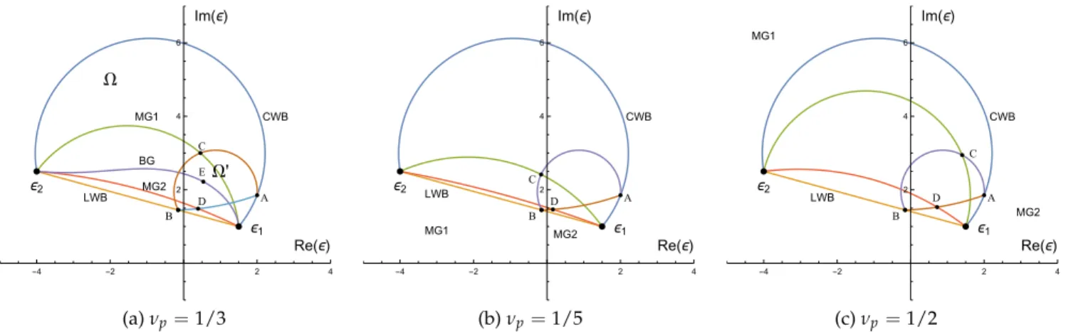
Fig. 3.(color online) Illustration of the Wiener and Bergman-Milton bounds for a two-component mixture withǫ1 =1.5+1.0iand ǫ2 =−4.0+2.5i. Curves MG1, MG2 and BG are parametric plots of the complex functions(ǫMG)p[formula (34)] andǫBG[formula
(30)] as functions of ffor 0≤ f ≤1 and three different values ofνp, as labeled. Arcs ACB and ADB are parametric plots of(ǫMG)p
as a function ofνpfor fixedfand different choice of the host medium (hence two different arcs). Notations: LWB - linear Wiener
bound; CWB - circular Wiener bound; MG1 - Maxwell Garnett mixing formula in whichǫh =ǫ1,ǫi =ǫ2andf = f2; MG2 - same
but forǫh = ǫ2,ǫi = ǫ1andf = f1, BG - symmetric Bruggeman mixing formula; A, B, C, D, E mark the points on CWB, LWB,
MG1, MG2, BG curves for which f1 = 0.7 and f2 = 0.3. Point E and curve BG are shown in Panel (a) only. Only the curves MG1
and MG2 depend onνp. The regionΩ(delineated by LWB and CWB) is the locus of all points(ǫeff)pthat are attainable for the
two-component mixture regardless off1andf2;Ω′(between the two arcs ACB and ADB) is the locus of all points that are attainable for
this mixture andf1=0.7,f2=0.3.
straight line and another a circle that crossesǫ1,ǫ2and the
ori-gin (three points define a circle). We only need a part of this circle - the arc that does not contain the origin. The two lines can be obtained by plotting parametrically the complex func-tionsη(f) = fǫ1+ (1−f)ǫ2andζ(f) = [f/ǫ1+ (1−f)/ǫ2]−1
for 0≤ f ≤1 and are marked in Fig.3as LWB (linear Wiener bound) and CWB (circular Wiener bound).
The closed areaΩ(we follow the notations of Milton [30])
be-tween the lines LWB and CWB is the locus of all complex points
(ǫeff)pthat can be obtained in the two-component mixture. We
can say thatΩisaccessible. This means that, for any pointξ∈Ω,
there exists a composite with(ǫeff)p =ξ. The boundary ofΩis
also accessible, as was demonstrated with the example of one-dimensional medium in Sec.5. However, all points outsideΩ
are not accessible - they do not correspond to(ǫeff)pof any
two-component mixture with the fixed constituent permittivitiesǫ1
andǫ2.
We do not give a mathematical proof of these properties of
Ωbut we can make them plausible. Let us start with a one-dimensional, periodic in theZ direction, two-component lay-ered medium with some volume fractionsf1andf2. The
princi-pal value(ǫeff)zfor this geometry will correspond to a point A
on the line CWB and the principal values(ǫeff)x = (ǫeff)ywill
correspond to a point B on LWB. The points A and B are shown in Fig.3for f1 = 0.7 and f2 =0.3. We will then continuously
deform the composite while keeping the volume fractions fixed until we end up with a medium that is identical to the original one except that it is rotated by 90◦in theXZplane. In the end state,(ǫeff)xwill correspond to the point A and(ǫeff)y= (ǫeff)z
will correspond to the Point B. The intermediate states of this transformation will generate two continuous trajectories [the loci of the points(ǫeff)xand(ǫeff)z] that connect A and B and
one closed loop staring and terminating at B [the loci of the points(ǫeff)y]. Two such curves that connect A and B (the arcs
ACB and ADB) are also shown in Fig.3.
Now, let us scanf1andf2fromf1=1,f2=0 tof1=0,f2=
1. The points A and B will slide on the lines CWB and LWB from
ǫ1toǫ2, and the continuous curves that connect them will fill
the regionΩcompletely while none of these curves will cross
the boundary ofΩ. On the other hand, while deforming the composite between the states A and B, we can arrive at a com-posite of an arbitrary three-dimensional geometry modulo the given volume fractions. Thus, for a two component medium with arbitrary volume fractions, we can state that (i)(ǫeff)p ∈Ω
and (ii) ifζ∈Ω, then there exists a composite with(ǫeff)p=ζ.
We now discuss the various curves shown in Fig.3in more detail.
The curves marked as MG1, MG2 display the results com-puted by the Maxwell Garnett mixing formula (34) with vari-ous values ofνp, as labeled. MG1 is obtained by assuming that
ǫh =ǫ1,ǫi =ǫ2, f = f2. We then take the expression (34) and
plot(ǫMG)pparametrically as a function of ffor 0≤ f ≤1 for
three different values ofνp. MG2 is obtained in a similar fashion
but usingǫh=ǫ2,ǫi=ǫ1, f =f1.
Notice that, at each of the three values ofνpused, the curves
MG1 and MG2 do not coincide because (34) is not “symmetric” in the sense of (28). For this reason, MG1 and MG2 can not be accuratesimultaneouslyanywhere except in the close vicinities ofǫ1andǫ2. Since there is no reason to prefer MG1 over MG2
or vice versa (unlessf1orf2are small), MG1 and MG2 can not
be accuratein general, that is for any composite that is somehow compatible with the parameters of the mixing formula. This point should be clear already from the fact that composites that are not made of ellipsoids are not characterizable mathemati-cally byjust threedepolarization factorsνp.
However, in the limitsνp →0 andνp →1, MG1 and MG2
coincide with each other and with either LWB or CWB. In these limits MG1 and MG2 are exact.
In Panel (a), we also plot the curve BG computed according to (30) with the “+” sign. This BG curve follows closely MG1 in the vicinity ofǫ1and MG2 in the vicinity ofǫ2. This result is
approxima-tions coincide to first order inf: see (31) and recall that f = f2
for MG1 andf = f1for MG2.
The two arcs ACB and ADB that connect the points A and B are defined by the following conditions: if continued to full cir-cles, ACB will crossǫ1and ADB will crossǫ2. The arcs can also
be obtained by plotting(ǫMG)pas given by (34) parametrically
as a function ofνpfor fixedf1and f2. To plot the arc ACB, we
setǫh=ǫ1,ǫi=ǫ2andf= f2in (34), just as was done in order
to compute the curve MG1. However, instead of fixingνpand
varying f, we now fix f=0.3 and varyνpfrom 0 to 1. Similarly,
the arc ADB is obtained by settingǫh=ǫ2,ǫi=ǫ1, f = f1and
varyingνpin the same interval.
The region delineated by the arcs ACB and ADB is denoted byΩ′. It is important for the following reason. Above, we have
defined the regionΩ, which is the locus of all points(ǫeff)pfor
the two-component mixture regardless of the volume fractions. If we fix the latter to f1andf2, the region of allowed(ǫeff)pcan
be further narrowed. It is shown in Refs. [29,30] that this region is preciselyΩ′. Note that the Maxwell Garnett approximation (34) with the same f1and f2yields the results on the boundary
ofΩ′. Conversely, any point on the boundary ofΩ′corresponds to (34) with someνp. The isotropic Bruggeman’s solution is
safely insideΩ′- see point E in Panel (a).
Just likeΩ, the regionΩ′is also accessible. This means that
each point insideΩ′ corresponds to a certain composite with
given ǫ1, ǫ2, f1 and f2. However, it is not obvious how the
boundaries ofΩ′ can be accessed. Above, we have seen that
the boundaries ofΩare accessed by the solutions to the
homog-enization problem in a very simple one-dimensional geometry wherein the smooth fieldScan be easily (and precisely) defined. The same is true forΩ′. It can be shown [29] that the
geome-try for which the boundary ofΩ′is accessed is an assembly of coated ellipsoids that are closely packed to fill the entire space. This is possible if we take an infinite sequence of such ellipsoids of ever decreasing size. Note that all major axes of the ellip-soids should be parallel, the core and the shell of each ellipsoid should be confocal, and the volume fractions of theǫ1 andǫ2
substances comprising each ellipsoid should be fixed tof1and f2. The arrangement in whichǫ1is the core andǫ2is the shell
will give one circular boundary ofΩ′and the arrangement in whichǫ2is in the core andǫ1 is in the shell will give another
boundary.
Of course, the above arrangement is a purely mathematical construct, it is not realizable in practice. However, it is interest-ing t