Practical
Contamination
Management
From Processing
to Delivery
HYDAC FILTER SYSTEMS GMBH
Industriegebiet 66280 Sulzbach/Saar
Page 25 Page 26 Page 27 Page 28 Page 28 Page 28 Page 29 Page 31 Page 32 Page 35 Page 35 Page 36 Page 36 Page 40 Page 42 Page 42 Page 43 Page 45 Page 47 Page 49
Definition of
Contamination Management
Contamination Management
Basics
2.1 Definition of
Contamination Types
2.2 Consequences of
Particulate Contamination
in Power Fluid Systems
2.3 Classification of
Particulate Contamination
in Fluids
2.3.1 ISO 4405 —
“Hydraulic Power Fluid —
Fluid Contamination —
Determining Particulate
Contamination Employing
Gravimetric Analysis Methods”
2.3.2 ISO 4406:1999
2.3.3 NAS 1638
2.3.4 SAE AS 4059
2.3.5 Procedure in Evaluating
Fluid Samples According to
ISO 4406:1999, NAS 1638
and SAE AS 4059
Determining the
Residual Dirt Quantity
of Components
3.1 Ultrasonic Method
3.2 Flushing Method
3.3 Shaking Method
3.4 Evaluation Methods
Analysis of the Cleanliness
of Systems
on the Flushing/
Test Stand
4.1 Turbulent Flow
4.2 Dispersion Effect
4.3 Flushing of All Ducts
and Surfaces
4.4 Pulsating Flow
during Flushing
1
2
3
4
Page 3 Page 5 Page 5 Page 8 Page 12 Page 13 Page 14 Page 15 Page 16 Page 17 Page 19 Page 19 Page 20 Page 20 Page 21 Page 23 Page 23 Page 24 Page 25 Page 254.5 Performing
a Cleanliness Check
on a Flushing Stand
4.5.1 Determining Overall System
Contamination
Contamination Monitoring
5.1 Planning and Design
5.2 How Sampling is Done
5.3 Inspection of the
Manufacturing and Assembly Line
5.4 Results
Drafting
a Cleanliness Specification
6.1 Establishing
Cleanliness Specifications
Sources of Contamination in the
Manufacturing and Assembly of
Hydraulic Systems
7.1 Preventing the Ingression
of Contamination in the
Manufacturing and Assembly
of Hydraulic Systems
7.2 Removal of
Particulate Contamination
from Hydraulic Systems
(Practical Experience)
and Components
7.2.1 Cleaning System
7.2.2 Function Testing
7.3 Storage, Logistics
and Ambient Conditions
7.4
Supplier Parts and Components
Manufactured In-house
Commissioning Flushing
Economic Efficiency Analysis
Contamination Management
in Practice
Reference List
5
6
7
8
9
10
E 7.604.1/05.091
Definition of
Contamination
Management
Contamination management pertains to the analysis and optimization of processes with regard to the cleanliness of
components, systems and the purity of the fluids employed. In today’s hydraulic systems — in the automotive industry and their suppliers, the hydraulics and mobile hydraulics industry — smaller, lighter and more powerful components are currently being employed as compared to say 10 years ago. The use of these components also means that the demands made of system
cleanliness are now much higher, as has been shown by various studies. Between 70-80 % of hydraulic system outages is due to increased contamination. This failure rate not only applies to the classic hydraulics industry. Contamination
Management is also a key issue in the automotive industry, in which the use of electrohydraulic systems is on the rise. In this context, hydraulic or fluid power systems are used in a general sense for all industries (automotive, hydraulics and mobile hydraulics industries). Cleanliness specifications are currently applied in the automotive industry for the following:
motors (fuel and oil supply systems)
power steering
manual/automatic transmissions electrohydraulic systems (suspension, clutch, brake, ABS and ESP systems)
central hydraulic systems
This list is by no means exhaustive and is intended rather as a sample of the areas in which contamination management plays a role.
In the past, power fluid systems were equipped with system filtration which cleaned the system during commissioning and then had the task of maintaining system fluid cleanliness at a constant level, e.g. by using commissioning filters and initial brief maintenance intervals followed by changing over to system filtration. This approach frequently no longer suffices due to the growing demands made of today’s hydraulic systems (extended maintenance intervals and mounting cost pressure). Precommissioning flushing is performed in large systems in the hydraulics industry to quickly bring the contamination level down to an acceptable level.
However, in small, mass-produced hydraulic systems (e.g. in the automotive and hydraulics industries) this is not always possible. That is why
contamination management begins with the manufacture of the individual components and extends throughout the entire process chain up to and including the finished component. Ideally, the design and development departments are also integrated in this process so that component design facilitates the washing of components in a cost-efficient manner. Suppliers also have to be involved in
contamination management when the manufacturing process involves a large portion of sourced
components. By introducing contamination management with a view to minimizing particulate concentration in all areas, beginning with manufacturing and extending to the operation of the entire system, system malfunction and failure caused by particulate contamination can be prevented and, as a result, costs savings achieved. Cutting the costs of machining tools, improving the utilization of test stations, and optimizing the use of washing machines can do this.
This results in the following contamination management tasks: development of systems which are optimized so as to facilitate cleaning
optimizing and monitoring washing and flushing processes
training employees and raising their awareness
detecting and eliminating sources of contamination
drafting analysis instructions drafting cleanliness specifications for components and systems An overall cost assessment is done to gauge the success of contamination management. The following factors are considered:
- warranty and non-warranty courtesy work
- energy costs - reworking costs - machining tool costs - operating costs of washing
machines and test stations - labor costs, etc.
The principles and applications of contamination management are detailed below.
Definitions:
Contamination management monitoring/optimization of cleanliness in material flows
and system assembly
Power fluid system hydraulic systems, including automotive systems containing
fluid fillings (e.g. motors, transmissions, power steering, ABS...)
Basic contamination quantity of contamination present subsequent to assembly
Ingress contamination particulate contamination caused by ingression
Initial damage damage to surfaces caused during function
testing/commissioning or assembly of systems
Contamination monitoring analysis of processes with regard to the ingress of dirt caused
by them
Online measurement measurement process in which the sample to be analyzed is
process fed to a measurement device directly from the system, e.g.
automatic particle counter of a hydraulic system
Offline measurement measurement process in which the sample is taken from the
process system and analyzed elsewhere, e.g. taking an oil sample
and sending it in to a laboratory
E
Contamination
Management
Basics
2.1
Definition of
Contamination Types
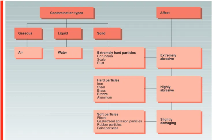
Various types of contamination occur in power fluid systems: gaseous (e.g. air), liquid (e.g. water) and solid contaminants.
An overview of the various contamination types is shown in the following diagram:
Fig. 1: Contamination Types
2
As you can tell from examining Figure 1, solid contamination is subdivided into three groups: extremely hard, hard and soft particles. Extremely hard particles can cause substantial damage in power fluid systems if they are not removed as quickly as possible. Preventive measures can reduce the ingress of contaminants in systems.
Hard particles are frequently listed separately in specifications. Maximum values are specified for the longest dimension these hard particles may have, e.g. largest abrasive particle: max. 200 µm or 200 x 90 µm or no particles > 200 µm.
Not only the hardness of
contamination particles play a role but also their number and size distribution as well.
The particle size distribution in new systems is different from that of systems that have been in operation for a number of hours. In new systems, there is an accumulation of coarse contaminants up to several millimeters long, which are then increasingly reduced in size in the course of operation or eliminated by filtration. After several hours of operation most particles are so small that they are no longer visible to the naked eye.
When commissioning power fluid systems there is additional particulate contamination by virtue of abrasive wear in which rough edges are worn away through running-in. Contamination management can’t prevent this ingress of contaminants, however if basic contamination is lower there is less abrasion during system startup.
Fig. 2
As the above diagram shows, the level of contamination without contamination management is higher throughout system operation as compared to a system in which contamination management is employed, the result being that more initial damage may be caused to surfaces.
E
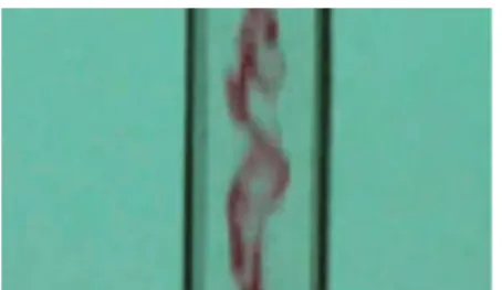
The following microscope images show typical particle samples as occur in power fluid systems.
Fig. 3
Sample containing coarse particles
Sample containing fine particles
An average healthy human eye can see items down to ca. 40 µm in size. Particle analyses are conducted using a microscope or in power fluid systems using particle counters employing the light extinction principle (cf. section 2.3.5).
2.2
Consequences of
Particulate Contamination
in Power Fluid Systems
Particulate contaminants circulating in power fluid systems cause surface degradation through general mechanical wear (abrasion, erosion, and surface fatigue).
This wear causes increasing numbers of particles to be formed, the result being that wear
increases if the “chain reaction of wear” is not properly contained (by reducing contamination). Gaps grow larger, leakage oil flows increase in size, and operating efficiency (e.g. of pumps) decreases. Metering edges are worn away, thus resulting in control inaccuracies. In some cases, blockage of control ducts or nozzle bores occurs.
The chain reaction of wear during the everyday operation of hydraulic systems has to be interrupted by properly designed and
dimensioned filter systems. However, the measure of security afforded the user is deceptive as highly damaging contaminants seep in during component and system assembly and system installation. This ingress of contaminants not only can cause preliminary damage to system components but also premature failure as well.
Generally speaking, system filtration concepts are not designed to adequately deal with large quantities of dirt as occur in connection with: component machining
system assembly system filling commissioning system repair work Fig. 5
Examples of Wear to Movable Surfaces
E
A study conducted by the University of Hanover describes the factors impacting the fatigue life of roller bearings as follows: “The quantity of contamination in the lubricant is described by the particle quantity and size. Combining this with particle hardness and geometry results in the type and extent of damage to raceways, with the extent also being affected by the elasto-plastic behavior of the material. The amount of damage is determined by the quantity of particles in the lubrication gap and the rollover frequency. Continued rollover leads to cracking, which in the form of fatigue damage (pitting) leads to roller bearing damage (bearing failure).”
Fig. 6
Factors Affecting Roller Bearing Life (1)
In practice ball bearings with their punctiform contact are shown in most cases to be less sensitive to particulate contamination than roller bearings with their linear contact. Friction bearings with their larger lubrication gaps are the least sensitive to particulate contamination.
The following table provides an overview of the most common gap sizes:
Fig. 7
Component Typical critical clearance
[µm] Gear pump (J1, J2) 0.5 – 5 Vane-cell pump (J1) 0.5 – 5 Piston pump (J2) 0.5 – 1 Control valve (J1) 5 - 25 Servo valve (J1) 5 – 8
Comprehensive studies of particle distributions on components and in hydraulic systems have shown that at the beginning of a system’s life, i.e. during assembly and
commissioning, the particles are larger than during subsequent operation.
These large particles – up to several millimeters in size in part – can cause spontaneous outages: valve blockages
substantial preliminary damage to pumps
destruction of seals and gaskets followed by leakage
Active contamination management enables this rate can be reduced and costs accordingly cut, i.e. costs caused by production stops costs caused by delays in commissioning systems costs incurred by longer testing periods since a flushing cycle is required to remove integral contamination
warranty costs reworking costs
E
Fig. 8
Destroyed Raceway of a Ball Bearing Caused by Particulate Contamination
Fig. 9
Chip Embedded in the Surface of a Friction Bearing
Contamination management counters the situation as follows: In new systems the individual components are brought to a uniform cleanliness level, the filling fluid is kept at a defined level, as is the fluid during system operation (cf. Contamination Monitoring, section 5 ff.).
2.3
Classification of
Particulate Contamination
in Fluids
The objective of the procedures described below is to enable a reproducible classification of particulate contaminants in fluids. Currently there are 4 procedures for classifying particulate contaminants in fluids: Standard Application Parameters Analysis methods Remarks ISO 4405 Highly contaminated media, e.g. washing media, machining fluids
[mg/liters of fluid]
In this lab method, 1 liter of the fluid undergoing analysis is filtered through a prepared membrane, which is then weighed
Very time-consuming method ISO 4406:1999 Hydraulic fluids Lubrication oils Number of particles > 4 µm (c) > 6 µm (c) > 14 µm (c) NAS 1638 Hydraulic fluids Lubrication oils Number of particles 5 – 15 µm 15 – 25 µm 25 – 50 µm 50 – 100 µm > 100 µm SAE AS 4059 Hydraulic fluids Lubrication oils Number of particles > 4 µm (c) > 6 µm (c) > 14 µm (c) > 21 µm (c) > 38 µm (c) > 70 µm (c) 1. Manual evaluation:
The fluid undergoing analysis is filtered through a prepared membrane and the cleanliness class (contamination rating) estimated or counted by hand using a microscope.
2. Automated particle counting:
The fluid undergoing analysis is conducted through a particle counter, which tallies the particle fractions.
1. Manual evaluation:
Very time-consuming, not very exact.
2. Automated particle counting:
Result available almost immediately. These standards are described
in detail below.
E
Afterwards the membrane is weighed and this value recorded as m (T).
Now the membranes are fixed in the membrane retainer and the fluid undergoing analysis is filtered. This is followed by flushing off the contaminant on the membrane using filtered solvent to completely remove the contaminant. When analyzing oil-laden fluids it is important that the remaining oil is completely flushed off the membrane.
This is followed by drying the membrane, cooling and weighing it (as described above). The measured value is now recorded as m (E). Gravimetric contamination is calculated as follows: M (G) = m(E) – m(T)
2.3.1
ISO 4405 – “Hydraulic
Power Fluid –
Fluid Contamination –
Determining Particulate
Contamination Employing
Gravimetric Analysis
Methods”
This international standard describes the gravimetric method for determining the particulate contamination of hydraulic fluids. Basic principle:
A known volume of fluid is filtered through one or two filter disks using vacuum action and the weight differential of the filter disks (upstream and downstream of filtration) measured. The second membrane is used for evaluating accuracy.
In order to determine the gravimetric contamination of the fluid, a representative sample has to be taken from the system. ISO 4405 describes the cleaning procedure for the equipment being used. It also describes the preparatory procedures for the analysis membranes:
The membranes are flushed with isopropanol prior to use, dried in a drying oven until they achieve a constant weight, and then cooled in a defined dry environment. It is important that cooling takes place in a defined dry environment,
otherwise the membrane absorbs moisture from the surroundings, thus skewing the final result.
2.3.2
ISO 4406:1999
In ISO 4406, particle counts are determined cumulatively, i.e. > 4 µm (c), > 6 µm (c) and > 14 µm (c) (manually by filtering the fluid through an analysis membrane or automatically using particle counters) and allocated to measurement references. The goal of allocating particle counts to references is to facilitate the assessment of fluid cleanliness ratings.
In 1999 the “old” ISO 4406 was revised and the size ranges of the particle sizes undergoing analysis redefined. The counting method and calibration were also changed. This is important for the user in his everyday work:
Even though the measurement references of the particles
undergoing analysis have changed, the cleanliness code will change only in individual cases. When drafting the “new” ISO 4406 it was ensured that not all the existing cleanliness provisions for systems
had to be changed (Lit.©HYDAC,
“Filters – Power Fluid Technology, New Test Dust, New Calibration, New Filter Testing Methods — How This Impacts Everyday Work”).
Overview of the changes:
If the number of particles counted in the sample is larger than 20, the
result has to be reported with≥.
Note: increasing the measurement reference by 1 causes the particle count to double.
Example:
ISO class 18 / 15 / 11 says that the following are found in 1 ml of analyzed sample: 1,300 – 2,500 particles > 4 µm (c) 160 – 320 particles > 6 µm (c) 10 – 20 particles > 14 µm (c) Fig. 11 Microscopic Examination of an Oil Sample (100 ml) Magnification 100x (ISO 18 / 15 / 11) Allocation of particle counts to
cleanliness classes:
No. of particles/ml Cleanliness class Over Up to 2,500,000 > 28 1,300,000 2,500,000 28 640,000 1,300,000 27 320,000 640,000 26 160,000 320,000 25 80,000 160,000 24 40,000 80,000 23 20,000 40,000 22 10,000 20,000 21 5,000 10,000 20 2,500 5,000 19 1,300 2,500 18 640 1,300 17 320 640 16 160 320 15 80 160 14 40 80 13 20 40 12 10 20 11 5 10 10 2.5 5 9 1.3 2.5 8
The reproducibility of the results in cleanliness class 8 depends on the concentration of particles in the sample undergoing analysis.
Size ranges Dimension determined Test dust Comparable size ranges “old” ISO 4406:1987 > 5 µm, > 15 µm Longest dimension of a particle ACFTD dust Old ACFTD calibration > 4 µm (c) > 6 µm (c) > 14 µm (c) Diameter of the area-equivalent circle ISO 11171:1999 ISO 12103-1A1 ISO 12103-1A2 ISO 12103-1A3 ISO 12103-1A4 New NIST calibration 4 µm (c) 6 µm (c) 14 µm (c) “new” ISO 4406:1999 1-10 µm Ultrafine fraction SAE Fine, AC Fine SAE 5-80 µm ISO MTD Calibration dust for particle counters SAE Coarse Coarse fraction Comparable ACFTD dusts < 1 µm 4.3 µm 15.5 µm 1,300 – 2,500 particles > 4 µm (c) 160 – 320 particles > 6 µm (c) 10 – 20 particles > 14 µm (c) E 7.604.1/05.09
2.3.3
NAS 1638
Like ISO 4406, NAS 1638 describes particle concentrations in liquids. The analysis methods can be applied in the same manner as ISO 4406:1987. In contrast to ISO 4406, certain particle ranges are counted in NAS 1638 and attributed to measurement references. The following table shows the cleanliness classes in relation to the particle concentration analyzed:
Increasing the class by 1 causes the particle count to double on average. The particle counts of class 10 are bold-faced in the above table.
Fig. 12 Microscopic Examination of an Oil Sample (100 ml) Magnification 100x (NAS 10) Particle size [µm] 5-15 15-25 25-50 50-100 >100
No. of particles in 100 ml sample
00 125 22 4 1 0 0 250 44 8 2 0 1 500 89 16 3 1 2 1,000 178 32 6 1 3 2,000 356 63 11 2 4 4,000 712 126 22 4 5 8,000 1,425 253 45 8 6 16,000 1,850 506 90 16 7 32,000 5,700 1,012 180 32 8 64,000 11,600 2,025 360 64 9 128,000 22,800 4,050 720 128 10 256,000 45,600 8,100 1,440 256 11 512,000 91,200 16,200 2,880 512 12 1,024, 000 182,400 32,400 5,760 1,024 Cleanliness class
2.3.4
SAE AS 4059
Like ISO 4406 and NAS 1638, SAE AS 4059 describes particle
concentrations in liquids. The analysis methods can be applied in the same manner as ISO 4406:1999 and NAS 1638. The SAE cleanliness classes are based on particle size, number and distribution. Just like for the ISO classification, the different particle concentrations are assigned numerical codes (see table). Compared to the 3-digit ISO code, in which the particle size ranges
are fixed (> 4 µm(c)/ > 6 µm(c)/
>14µm(c)), the SAE cleanliness
class assigns the capital letters A-F to the particle size range being considered.
These letters correspond to
> 4 µm(c)... > 70 µm(c).
The following table shows the cleanliness classes in relation to the particle concentration determined:
** Particle sizes determined according to the diameter of the projected area-equivalent circle. * Particle sizes measured according to the longest dimension.
A B C D E F 000 195 76 14 3 1 0 00 390 152 27 5 1 0 0 780 304 54 10 2 0 1 1,560 609 109 20 4 1 2 3,120 1,220 217 39 7 1 3 6,250 2,430 432 76 13 2 4 12,500 4,860 864 152 26 4 5 25,000 9,730 1,730 306 53 8 6 50,000 19,500 3,460 612 106 16 7 100,000 38,900 6,920 1,220 212 32 8 200,000 77,900 13,900 2,450 424 64 9 400,000 156,000 27,700 4,900 848 128 10 800,000 311,000 55,400 9,800 1,700 256 11 1,600,000 623,000 111,000 19,600 3,390 1,020 12 3,200,000 1,250,000 222,000 39,200 6,780
Maximum Particle Concentration [particles/100 ml]
> 1 µm > 5 µm > 15 µm > 25 µm > 50 µm > 100 µm > 4 µm (c) > 6 µm (c) > 14 µm (c) > 21 µm (c) > 38 µm (c) > 70 µm (c) Size ISO 4402 Calibration or visual counting* Size ISO 11171, Calibration or electron microscope** Size coding
The SAE cleanliness classes can be represented as follows:
1. Absolute particle count larger than a defined particle size
Example:
Cleanliness class according to AS 4059:6
The maximum permissible particle count in the individual size ranges is shown in the table in boldface. Cleanliness class according to AS 4059:6 B
Size B particles may not exceed the maximum number indicated for class 6.
6 B = max. 19,500 particles of a size of 5 µm or 6 µm (c)
2. Specifying a cleanliness class for each particle size
Example:
Cleanliness class according to AS 4059: 7 B / 6 C / 5 D Size B (5 µm or 6 µm (c)): 38,900 particles / 100 ml Size C (15 µm or 14 µm (c)): 3,460 particles / 100 ml Size D (25 µm or 21 µm (c)): 306 particles / 100 ml
3. Specifying the highest cleanliness class measured
Example:
Cleanliness class according to AS 4059:6 B – F
The 6 B – F specification requires a particle count in size ranges B – F. The respective particle
concentration of cleanliness class 6 may not be exceeded in any of these ranges.
E
2.3.5
Procedure in Evaluating
Fluid Samples According
to ISO 4406:1999,
NAS 1638 and
SAE AS 4059
A representative sample is taken of the fluid and analyzed as follows:
1. Manual procedure according
to ISO 4407(Hydraulic fluid power
– Fluid contamination – Determination of particulate contamination by the counting method using a microscope). ISO 4407 contains a description of a microscopic counting method for membranes. 100 ml of the sample undergoing analysis is filtered through an analysis membrane featuring an average pore size of < 1-µm and square markings. The standard also describes the cleaning procedure and maximum particle count of the negative control.
After the analysis membranes are dried, 10, 20 or 50 squares are counted depending on the size of the particles, followed by adding the values and extrapolating to the membrane diameter.
The manual count of the particles is done in the “old” levels of > 5 µm and > 15 µm since the longest dimension of a particle is counted in ISO 4407 yet the diameter of the area-equivalent circle is counted in the “new” ISO 4406:1999. As described above, the reference values obtained for this count correspond to the reference values of the “new” evaluation.
Fig. 13
This counting method can only be used for very clean samples. Generally speaking, the cleanliness classes are estimated on the basis of reference photographs or the samples automatically counted.
2. Automated particle counting
Below follows a description of how common particle counters
employing the light extinction principle function.
The figure below shows a simplified rendering of the measurement principle employed in the light extinction principle. The light source transmits the monochromatic light through the oil flow onto a photodetector, which generates a specific electrical signal. A shadow is created on the photodetector if a particle (black) comes between the light source and the photodetector.
This shadow causes the electrical signal generated by the sensor to change. This change can be used to determine the size of the shadow cast by this particle and thus the particle size to be determined.
Fig. 14
This procedure enables the cleanliness classes according to ISO 4406:1987, ISO 4406:1999, NAS 1638 and SAE AS 4059 to be determined.
The “noise” involved in this measurement principle is extraneous liquids and gases which cause the light beam to be interrupted and thus be counted as particles.
The particle counter should be calibrated according to ISO 11943 (for ISO 4406:1999).
The following types of automatic particle counting are used: Online processes in which the sample is taken directly from the system and conducted into the particle counter, or the sensor is integrated directly in the system.
Or offline processes in which the sample is filled into a sample container from which the liquid is conveyed through a particle counter.
Laboratory Particle Counter with a Bottle Sampling Unit
BSU 8000 with FCU 8000 Online Particle Counter of the FCU 2000 Series Fig. 15
Fig. 16
E
Determining the
Residual Dirt Quantity
of Components
Determining the residual dirt quantities present on components can be done employing quantitative and qualitative factors.
Quantitative: • mg/component • mg/surface unit (oil-wetted surface) • mg/kg component weight no. of particles > x µm/component • no. of particles > x µm/surface unit (oil-wetted surface)
Qualitative: length of the largest
particle (subdivision into hard/soft) Components with easily accessible surfaces are components in which only the outer surface is of interest for the most part when performing residual dirt analyses. There are exceptions here, e.g. transmission and pump housings, as the internal surface is of interest. These components belong to group 1 and their surfaces are not easily accessible in most cases. Components in which the inner surfaces are examined or
preassembled assemblies belong to group 2; for the analysis procedure for this group, refer to section 4. There are two methods that can be used to determine the residual dirt of group 1 components:
3.1
Ultrasonic Method
The ultrasound method involves submitting the components to an ultrasonic bath, exposing them for a defined period of time at a defined ultrasonic setting and bath temperature. The particulate contamination is loosened by the exposure and then flushed off the component using a suitable liquid. The particle dispersion in the flushing liquid obtained in this manner is analyzed according to specified evaluation methods (cf. section 3.4).
The ultrasonic energy setting and the duration of exposure have to be indicated in reporting the result. The ultrasonic procedure is particularly suitable for small components in which all surfaces have to be examined. Cast components and elastomers should not be subjected to ultrasonic washing if possible as a risk is posed here of the carbon inclusions in the cast piece being dissolved, thus skewing the results. These effects have to be
ascertained prior to performing an ultrasonic analysis.
3.2
Flushing Method
Components with easily accessible surfaces or components in which only surface parts have to be examined are analyzed using the flushing method. This method involves flushing the surface undergoing analysis in a defined clean environment using an analysis fluid, which also has a defined cleanliness. A “negative control” or basic contamination control is performed prior to analysis in which all the surfaces of the environment, e.g. the collecting basin, are flushed and the value obtained reported as the basic contamination of the analysis equipment. The flushing fluid is then analyzed using the specified evaluation methods.
Fig. 17
3.3
Shaking Method
This method is very rarely used, as it is very difficult to reproduce manually. However, results are reproducible when automatic shakers such as those used in chemical laboratories are employed. The analyzed components are components subject to wear whose inner surfaces are to be analyzed (e.g. pipes, tanks). The important thing is that the particles are flushed out of the inside of the components after being shaken.
The following table shows a comparison of the various methods for analyzing components and assemblies.
The areas shown inredare the
flushing areas; those shown in
bluethe designated analysis area.
In reality these two circuits are configured using suitable valves in such a manner that switchover can be done between the two storage tanks. The figure represents a simplified circuit diagram.
The analysis fluid is subjected to a pressure of ca. 4-6 bars and thus conveyed through the system filter and the spray gun into the analysis chamber. The system filter ensures that the analysis fluid sprayed on the surface being examined has a defined cleanliness. The particle-loaded fluid collects in the collecting basin and is filtered through the analysis membrane via vacuum action. The membrane is then evaluated according to the analysis methods described below.
Flushing method Components are flushed with the analysis fluid in a defined clean environment.
Components in which only surface parts have to be examined and components in which ultrasound may damage the surfaces.
Components with a simple design and with easily accessible surfaces. Analysis can be performed quickly Reproducibility Standards are not yet available (currently in preparation)
Ultrasonic method Components are exposed to an ultrasonic bath and are then flushed with the analysis fluid.
Small components and components in which all surfaces are to be analyzed (the component size depends on the ultrasonic bath).
Reproducibility Analysis takes a long time The energy acts on the surface undergoing analysis The surface has to be flushed No valid standards Applications How performed Cons Pros E 7.604.1/05.09
3.4
Evaluation Methods
Evaluating particle-laden flushing fluids can be done according to various criteria. Gravimetric analysis is useful for heavily contaminated components, whereas particle counts in various size ranges are useful for very clean components. The following table provides an overview of the individual evaluation methods:
The following table provides an overview of applications of the analysis and evaluation methods:
Evaluation Analysis method Simple components Components Complex components Simple systems Systems Complex systems easy-to-access surfaces gears internal surfaces pipes, tanks Components featuring various bore holes or ducts control plates surface is to be analyzed immersed sensors internal surfaces rails of common rail systems valves, pumps e.g. e.g. e.g. e.g. e.g. e.g.
Flushing Ultrasonic Flushing Ultrasonic Function testing*
method method U U U U NU U NU U NU CU** CU** NU CU** NU U U U U U NU CU** NU CU** NU U CU** NU CU** NU U
Gravimetry
Particle counting
U= usable
CU= conditionally usable
NU= not usable
*= section 4, Analysis of the Cleanliness of Systems on the Flushing/Test Stand.
**= It has to be ensured that the particles dislodged from the component can be flushed away.
E
Analysis of the
Cleanliness of
Systems on the
Flushing/Test Stand
The cleanliness of components and systems that pass through a flushing or test stand can be determined on the basis of the cleanliness of the test fluid in some cases. This indirect analysis method is preceded by manual analyses for validation purposes. For example, hoses are flushed by hand and the results evaluated in accordance with the methods discussed in section 3. At the same time, the cleanliness of the test fluid of the test stand is determined in the return flow, i.e. downstream of the component.
If a correlation is detected between the manual and the automatic (indirect) value, this means that indirect value analysis can be selected as a measure of quality. The flushing stand used for analyzing the residual dirt content of systems has to feature the following:
1. Flushing has to be done using as turbulent a flow as possible. 2. The fluid used has to posses a dispersion effect.
3. All channels and surfaces have to be exposed to the flow.
4. The effectiveness of flushing can be improved by pulsating the flushing.
4.1
Turbulent Flow
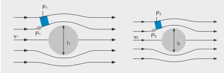
Reynolds NumberThe Reynolds number — a dimensionless reference — describes the flow properties of fluids. Below follows a brief description of how the Reynolds number is derived using pipe flow as an example.
Weights are discounted in the calculation of the Reynolds number. Generally speaking, only pressure, friction and inertial forces affect fluid elements and bodies subjected to flows. They have to be in balance at all points of the flow. If the relationship of friction and inertial forces is the same in similar points P1 and P2, then similar flows are said to be present.
Fig. 18 Similar Flows
Around Different Cylinders
The Reynolds equation looks like this when the above properties are taken into account:
Whereby: Q = volumetric flow rate (l/min)
v = viscosity (mm2/s)
and
d = inside pipe diameter (mm)
Re = mean velocity * internal pipe diameter
kinematic viscosity
Q di * v Re = 21220*
The critical Reynolds numberRecrit
depends on kinematic velocity v, flow rate Q of the fluid, and the geometry of the passage through the flow is being conducted. If the Reynolds number of a flow is smaller
thanRecrit, the flow is said to be
laminar.Turbulentflow is said to
be present for values aboveRecrit.
The critical Reynolds number for oil is given below.
Re crit oil = 1900 – 3000
(Source: Kahrs, M.: Der Druckverlust in Rohrleitungen ölhydraulischer Antriebe; VDI Forschungsheft 537, Düsseldorf 1970)
4
The following diagrams show the difference between laminar and turbulent flow.
Fig. 19
Laminar Flow
All particles move without mixing.
The path of a particle is described by a stream thread.
Parabola-shaped velocity distribution (applies to pipes).
Reynolds number smaller thanRecrit
Turbulent Flow
All particles are continuously mixed.
The path of a particle cannot be predicted.
Relatively even time-averaged velocity distribution (flattened parabola).
Reynolds number larger thanRecrit
The above diagram shows a
parabolic,laminar flowin a pipe.
This shows that the flow velocity of a laminar current in the middle of the pipe (peak of the parabola) is larger than along the pipe wall.
In aturbulent flowthis parabola
flattens and spreads (when mean values are considered), as
transversal currents are involved in a turbulent flow. They cause the flow velocity to be increased in the vicinity of the pipe walls.
This effect is utilized when flushing systems as increasing the flow rate causes particles that have been deposited on the wall to be loosened and swept away.
Source:
University of Würzburg Fluid Mechanics lecture
4.2
Dispersion Effect
The oil used for flushing has to have a dispersion effect so that particles are dislodged and transported off. Special thin-bodied mineral-oil-type flushing oils can contribute instrumentally to improving the flushing effect. They lower the adhesion force between the dirt particles and the pipe wall. By virtue of their excellent surface wetting properties, they creep into between the dirt particles and the wall, thus causing the particles to become dislodged. Experiments have shown that by changing the flushing fluid from an operating fluid to a flushing oil,
component/system cleanliness can be increased by a factor of 4. Flushing oils of this type have to then be closely matched to the hydraulic medium used as failure to properly match the two may lead to the following:
marked foaming filter blockage
clogging of the system
E
4.3
Flushing of All Ducts
and Surfaces
When setting up the inspection and testing plan, it has to be ensured that all surfaces and ducts are wetted during flushing.
4.4
Pulsating Flow during
Flushing
Pulsating flow or the reversal of the flow direction also results in improved removal of adhesive particles. In so doing, the main effect is achieved by virtue of alternating forces being applied to the particles to be dislodged. The same effect can be achieved via ultrasonic equipment or other vibration-generating equipment.
Fig. 20
The flushing of pipework/hoses and hydraulic systems can be done using a HYDAC Flushing Unit. The following is performed: Pressure testing
Flushing
Documentation of the flushing results
4.5
Performing a Cleanliness
Check on a Flushing
Stand
The cleanliness of components and systems which undergo function testing can be determined on a flushing or function test stand (= flushing stand).
This method is used for pumps, cylinders, transmissions, control units, power steering units, valve blocks, etc.
Once it is ensured that the flushing stand possesses the properties indicated above, an analysis is conducted as described below. Prior to the analysis the flushing stand is cleaned to a defined high cleanliness level so that the basic contamination of the test system does not affect the measurement results. Then this basic cleanliness is computed and recorded.
4.5.1
Determining Overall
System Contamination
The sampling site for an automatic particle counter is defined as a site upstream or downstream of the test item, which is subjected to a direct flow. The following is performed if the analysis result is to be additionally subjected to gravimetric analysis:
the entire test fluid is collected and filtered through an analysis membrane
or an inline membrane retainer featuring the analysis membrane is integrated in the return-flow line. Now the test item is tested in accordance with the inspection and testing plan, during which the cleanliness classes are recorded. Example 1:
The schematic below shows the analysis performed on a pump test stand.
Fig.21
After 5 minutes of testing the pump speed is increased to the maximum speed. This causes particulate contamination to be dislodged. The system becomes increasingly cleaner. Particulate contamination is still being released after 1 hour of testing (standard test time: 10-15 min.), consequently the cleanliness of the return-line fluid (blue = downstream of the test item) never achieves the same cleanliness as upstream of the test item. This method is suitable for checking the cleanliness of items being delivered quickly and simply in series testing, documenting it and then concluding the flushing procedure when the target value is achieved. By integrating the measurement circuit in the manufacturing instrumentation and control system it is also possible to quickly detect any deviations and initiate suitable measures. The goal of continuous cleanliness
monitoring is to monitor process reliability with regard to system cleanliness upon delivery.
A specification like this also enables increased system contamination to be responded to quickly. If these measurements are only conducted once a day, a whole day’s output might be affected and have to be remedied. The result is unnecessary costs that can be avoided by integrating a continuous measurement procedure.
When conducting a reference measurement, the system is disassembled after the test run, if possible, and the individual components analyzed using the flushing method.
Example:
As-supplied condition: 17 / 15 / 12 according to ISO 4406:1999
1. Warning point: 18 / 16 / 13 for 3 successive measurements
2. Stop signal: When exceeding 18 / 16 / 13 limit cleanliness class
in 2 successive measurements.
E
Contamination
Monitoring
The reliability of hydraulic systems can be impacted heavily by particulate contamination during the running-in phase. The risk of outages during the first minutes or hours of operation is particularly high as the foreign particles introduced or created during the assembly process are still relatively large and can thus cause sudden outages. During continued operation, these large particles are ground into smaller ones, the result being that damage can be caused to the surfaces of system
components during this crushing process. The consequences are leakage, degraded output and efficiency, or a shortening of the component’s service life. In many cases, microfiltering is used to quickly clean the system fluid during commissioning. However, in the automotive sector this is not possible in systems integrated in cars (exceptions: transmissions and motors). This is where contamination monitoring is key in the manufacture and assembly of these systems. By implementing contamination management a major portion of particulate contamination introduced during manufacture and assembly can be removed. The result is cost savings by virtue of smaller performance deviations on test stands caused by the sudden clogging of particles in sensitive system components plus lower costs associated with warranty and non-warranty courtesy work. For more information, refer to section 9. Below follows a description of the goal, design and performance of a process audit.
Contamination monitoring extends to checking the cleanliness status of all manufacturing and assembly processes considered relevant in this connection. (cf. analysis methods, described in section 4) Proper preparation and informing all those involved are key in contamination monitoring.
5.1
Planning and Design
First, the objective of contamination monitoring is specified, e.g. Determining the current situation Checking fluctuations between batches
Checking washing processes Comparing the target with the actual situation
Determining the sampling point During the planning and design phase, the sampling points for components and taking liquid samples are determined using a production plan or operation sheet. The employees to be involved in contamination monitoring are informed of the objectives and procedures.
NOTE:
Manufacturing has to continue in the same manner, meaning that no additional cleanliness levels, etc. are to be integrated. The purpose of contamination monitoring is not to check the quality produced by the employees but rather determining the causes and sources of contamination.
The following schematic is an excerpt of a manufacturing line:
Fig. 22
The schematic above shows the manufacturing processes and the corresponding sampling points. However, in actuality sampling is more comprehensive, i.e. the description includes the number of the Minimess fittings at which sampling is done, for example.
5.2
How Sampling is Done
A representative sampling is taken of the fluids and components; the samples are stored so as to prevent any further contamination. Special sampling bottles are used for the fluid samples; the
components are stored in defined clean packaging.
The analysis is performed in accordance with the methods specified in sections 3 and 4 and the findings recorded.
5.3
Inspection
of the Manufacturing
and Assembly Line
Properly trained or experienced individuals while inspecting the manufacturing and assembly line can detect some sources of contamination. That is why such an inspection is conducted during the audit. The findings made during inspection are then compared with the results in hand.
E
5.4
Results
The contamination monitoring results describe the condition at the time at when sampling is done. The findings might look like this:
Fig. 23
Micro-photograph Analysis membrane
Particulate contamination of a
componentprior tostorage
This chart shows an excerpt of the housing manufacturing process. The component samples are taken upstream and downstream of the washing station. The findings show that the washing station performs well and that it is well positioned here. Subsequent storage is not being done properly as the portion of particulate contamination is almost double. Fig. 24 Fig. 25 Micro-photograph Analysis membrane Particulate contamination of a
componentafterbeing in storage
Drafting a Cleanliness
Specification
By applying a cleanliness specification to components and the system it can be ensured that as-supplied quality is constant. The following should be borne in mind when drafting a cleanliness specification:
State of the art Benchmarking — what do others do?
Inclusion of previous experience — if available —
Defining and implementing contamination management as an “official project”
Inclusion of all hierarchy levels Accurate documentation of how the specification was developed Developing clear-cut definitions Next, it has to be determined which components in the system are the most sensitive. Frequently it is not possible to achieve the same level of cleanliness throughout the system during assembly. If suitable filtration takes place
upstreamof the sensitive
components, an area of low-contamination-sensitive components can be defined upstream of this filtration and an area of highly contamination-sensitive components downstream of the filter.
These individual components or system areas should be subdivided into sensitivity areas.
A maximum particulate
contamination value is specified for each of these cleanliness
categories.
A car motor illustrates this subdivision below:
In addition, the fluid cleanliness ratings of the individual system and process fluids are defined.
Category A B C Designation low particle-sensitivity particle-sensitive
high particle sensitivity
Category A B C Motor area Air
Coolant water circuit Low-pressure oil circuit Diesel direct injection High-pressure oil circuit
Description
For the most part low-pressure systems with large gap tolerances Low-pressure systems with small gap tolerances High-pressure systems with small gap tolerances and with exacting demands made of safety and security systems
6
E
6.1
Establishing
Cleanliness Specifications
The following parameters are defined in the cleanliness
specifications for the components: 1. Goal of the cleanliness
specification 2. Applicability
(system designation) 3. Extent of inspection
and testing; inspection and testing cycles 4. Sampling
5. Analysis method 6. Evaluation method 7. Accuracy
8. Analysis fluids to be used 9. Documentation
10. Limit values
This specification has to be made for each individual system; consequently a few things are discussed which have to be borne in mind.
Work instructions concerning sampling, analysis and evaluation methods should be described in detail so as to ensure that sampling is always done in a uniform manner. In addition, the analysis results depend on the analysis fluid and method, particularly when it comes to component analysis. Documentation should be done using forms so that all the results are readily accessible. Example of a form for entering findings:
Example of a Cleanliness Specification
1. Goal of the
cleanliness specification
The goal in implementing this cleanliness specification is to achieve a constant level of cleanliness for system X.
2. Applicability
(system designation)
This specification applies to system X including its series A, B, and C. It extends to all components whether sourced or manufactured in house. It also specifies the system fluids of system X with regard to their cleanliness.
3. Extent of inspection and testing; inspection and testing cycles
5 samples/month of each component are to be taken and analyzed. If the supplier parts achieve a constant cleanliness value after 6 months, the sampling cycle can be extended to sampling every 2 or 3 months. An analysis of the entire (assembled) system is to be done at least once a week prior to delivery. Checking of the fluid cleanliness should optimally be done on a continuous basis.
4. Sampling
Sampling of components is to be done at goods receiving. Sampling of components is to be
representative; samples are to be packed in a dust-tight manner and sent in to the laboratory. The fluid samples are to be taken at the sampling points indicated in the inspection and testing plan, or an instrument to be connected directly.
5. Analysis method
The flushing method is to be used for component analysis. The surfaces of the component are flushed in a defined clean environment using x ml of the test fluid (XY) — which possesses a cleanliness of xx — under a pressure of z bars as specified by the inspection and testing plan. The flushed-off particulate contamination is collected on an analysis membrane and subjected to gravimetric analysis.
Representative samples are taken of the system fluids at the specified sampling points. All testing parameters are specified, i.e. the duration of testing, what is tested, the pressures, speeds. When conducting static inspection and testing, e.g. pressure testing in pipeline and hoses, make sure that a flushing effect is present so that the cleanliness of these
components can be determined, i.e. the static pressure test has to be followed by a dynamic flushing process in order to analyze the actual quantity of particles which is flushed out of the component.
6. Evaluation method
In the component analyses the analysis membrane is dried until it achieves a constant weight, and then cooled in a defined dry environment and weighed. This procedure is repeated subsequent to filtration. The weight differential indicates the “gravimetric
contamination” of the component. This is followed by visually
examining the analysis membranes through a microscope and
measuring the longest particles. Evaluation of the fluid samples is done in accordance with ISO 4405, ISO 4407, ISO 4406:1999 or NAS 1638.
7. Accuracy
The analysis equipment has to be brought to a residual dirt content of 0.2 mg prior to conducting the analysis so that the measurements taken of the component samples are sufficiently accurate. This is determined by performing a negative control, i.e. flushing the equipment without testing. When the result of the analysis drops below 0.5 mg, the batch size is to be increased and thus a mean value of the results computed.
8. Analysis fluids to be used
The following analysis fluid should be used for the component analyses: ABC-XX, with a cleanliness class of 14 / 12 / 9 and no particles > 40 µm.
E
The following cleanliness specifications apply to each of these classes (fictitious example).
The transmission components are subdivided into the individual categories below:
Group A: crankcase sump Group B: intermediate housing,
transmission housing, coupling flange Group C: valve plate,
valve housing, centering plate
Fluid samples:
At the end of the test run, the transmission fluid may not fall short a cleanliness rating of 17 / 15 / 13 (c) according to ISO 4406:1999. The system is to be operated using a
cleanliness rating of 18 / 16 / 14 (c) according to ISO 4406:1999.
11. Procedure to be followed in the event that the specification is not adhered to
The supplier components are to be returned to the supplier in the event that the specification is not adhered to. If this procedure results in production delays, the components will be cleaned and analyzed by us at the supplier’s expense.
Particle sizes Max. 4 particles > 500 µm Max. size: 400 µm No fiber bundles Max. 4 particles > 400 µm Max. size: 800 µm Fibers up to 4 mm Max. 4 particles > 200 µm Max. size: 1,000 µm Fibers up to 2 mm Gravimetry 20 mg / component 10 mg / component 5 mg / component Category A B C Description
For the most part low-pressure systems with large gap tolerances Low-pressure systems with small gap tolerances
High-pressure systems with small gap tolerances and exacting demands
Designation low particle-sensitivity particle-sensitive high particle sensitivity Category A B C 9. Documentation
The documentation of the results is to done using a result sheet (cf. sample).
10. Limit values
The components are subdivided into 3 cleanliness classes:
Sources of
Contamination in
the Manufacturing
and Assembly of
Hydraulic Systems
Particulate contamination can enter a power fluid system in various ways. The main sources of ingression are shown in the following diagram:
Fig. 26
Some of these sources of
contamination can be eliminated in a simple, cost-effective manner.
The following applies in
Contamination Management:
What isn’t allowed to enter the system doesn’t have to be removed.
wear special, lint-free clothing. The assembly equipment has to be properly cleaned so as to prevent the ingress of dirt here, too.
Raising the Awareness of Employees
In order to achieve the objective of “defined cleanliness of components and systems” it is important that employees at all levels be involved in this process. Frequently, a considerable savings potential is contained in the employees’ wealth of ideas and experience — particularly those working at assembly lines and in fabrication. Experience has shown that when employees are able to identify with the objective being striven for, they are more able to help in
implementing it quickly and effectively.
Environment — Air Cleanliness
In some cases it will be necessary to set up a clean room for the final assembly of very contamination-sensitive systems, e.g. fuel systems, brakes shock absorbers, etc. This has to be decided on a case-by-case basis. However, in many cases performing the measures described here suffices.
7.1
Preventing the Ingression
of Contamination in the
Manufacturing and
Assembly of Hydraulic
Systems
The ingression of contamination in the manufacturing and assembly of hydraulic systems can be
eliminated in a cost-effective manner in various process steps.
Storage and Logistics
When storing and transporting the components and systems care has to be exercised to make sure that they are properly sealed shut or well packed. Transportation and storage packing has to be in keeping with the cleanliness status of the individual components.
Assembly of Systems and Subassemblies
The assembly of these systems is to be done in accordance with system requirements. This means that the assembly and mechanical fabrication areas have to be separated if necessary in order to prevent the ingress of
contamination. The assembly stations have to be kept clean to a defined cleanliness and those
7
E
7.2
Removal of Particulate
Contamination from
Hydraulic Systems
(Practical Experience)
and Components
Generally speaking, particulate contamination is removed from a hydraulic system via filtration. Various types of filters are used depending on the amount and type of contamination.
Belt filter systems or bag filters are used when large quantities of contaminants are involved (e.g. washing machines, machine tools). These filters have the job of removing the major portion of contaminants (often in kg) from the system. These filter types are also used for prefiltration purposes. In most cases, these coarse filters do their job of “removing a lot of dirt from the system” very well.
However, microfiltering also has to be done if a constant defined high level of cleanliness of the system fluid is to be ensured.
Whereas microfiltration ensures quality, the job of coarse filtration is to control the quantity of contamination.
7.2.1
Cleaning System
Individual components are freed of clinging contamination in cleaning systems (particles, remainder of machining or corrosion protection fluids, etc.). Cleaning can be done by employing various mechanical methods (e.g. spraying, flooding, ultrasonic methods) using various cleaning fluids (aqueous solutions or organic solvents). The
temperature and duration of cleaning also have a decisive effect on the cleaning effect. These factors have to be carefully matched and optimally tuned in order for a favorable cleaning effect to be achieved in an economical amount of time.
Fig. 27
Various studies of washing processes have shown that some of these for the most part cost-intensive processes aren’t worthy of the name. Some people refer to washing processes as “particle distribution processes”. This “property” was detected in examinations of components sampled upstream and
Example: Pipeline flushing after bending
Fig. 28
Micro-photograph Analysis membrane
When purchasing washing systems, make sure to specify the component cleanliness to be achieved and the maximum contamination load of the washing fluid in terms of mg/l or a
cleanliness class.
Washing systems used to be subdivided into micro and micronic washing. This was a very imprecise definition of the cleaning
performance to be achieved. Nowadays the permissible residual dirt quantity of the cleaned
components is defined. Specifying these residual dirt quantities is done as follows: mg/component, mg/kg component, mg/surface units or particle concentrations in various size ranges. In addition, the maximum sizes of the particles are defined which can be on the washed component, e.g. max. 3 particles > 200 µm, no particles > 400 µm. These values cannot be achieved unless the factors indicated above are matched and fine-tuned. The following factors additionally have to be borne in mind: environmental protection and labor safety, local situation relating to space and power available, and the target throughout rate.
The cleanliness of the washing and flushing fluids also has a decisive impact on the cleaning
performance of the washing machine.
However, we are concerned here only with the maintenance of the washing and flushing fluids. Pipe has been sawed and washed
Fig. 29
Micro-photograph Analysis membrane
After sawing and washing, the pipe is bent and flushed.
There are two possible responses in a case like this:
1. Discontinue the washing process when component cleanliness becomes worse after washing than before.
Advantage:
temporary cost savings The best alternative: 2. Optimize the process
The following should particularly be borne in mind when optimizing washing processes:
cleanliness of the washing, flushing and corrosion protection fluid mechanical aspects
(e.g. clogged washing nozzles) suitability of the washing process for the components undergoing washing
filtration of the washing and flushing fluid
E
The following methods are used in standard maintenance:
The type and composition of the cleaning medium is to be taken into account in selecting the fluid maintenance options indicated above. When using ultrafiltration, it has to be borne in mind that separating out the cleaning substances cannot be avoided in certain cases. In addition, ultrafiltration can only be used for precleaned washing media since the performance of the separating membranes is degraded when they are loaded with particulate
contamination.
Using Filtration as Fluid Maintenance for Separating out Particulate Contamination
Bag and backflush filters in various microfilter ratings are the standard equipment used in the
maintenance of the fluid of washing systems. Although these filters are suitable for removing large quantities of contamination from a system, they are not suitable in most cases for maintaining defined cleanliness classes. Owing to their design, they do not offer much resistance; i.e. the counterpressure built up across the filter is very low, below 1 bar for the most part. That is why this filter type is frequently used in the main (full) flow when feeding cleaning fluid into the washing or flushing chamber. The filter housings are equipped with pressure gauges for monitoring the proper functioning of the filter. Bag filters pose the risk that
That is why it is advisable to additionally define minimum change intervals and to regularly monitor the cleanliness of the washing fluid in addition to the standard parameters like pH value or microbial count.
Residual dirt values of cleaned components are increasingly being defined and specified as an acceptance criterion for the cleaning system. It is of paramount importance that constant
adherence be maintained to these values. It is also imperative that the quality of the cleaning fluid be maintained at a constant, high level.
This can be achieved by the targeted use of microfilters featuring a constant, absolute separation rate. For the most part, tube filters or disk filters are used. The advantage offered by these filter types as compared to
standard hydraulic filter elements is their high contaminant retention rate owing to their depth effect. Thanks to the high contaminant separation rate offered by these filter types, they remove a high amount of contamination from the washing fluid; this causing the filters to become quickly exhausted and blocked.
A sufficiently long service life coupled with high washing fluid cleanliness can be achieved by combining filters for removing the main portion of contaminants from the system with absolute
A typical example is described below.
At a leading automotive supplier, the camshafts were to be cleaned to a defined cleanliness of
9 mg/component. Point of departure:
Challenge:
Clogging of the tank Quality no longer sufficient after 2-3 days
Fluctuation in the contamination content of the components upstream of the line: 30 – 50 mg Cleaning costs per component not
to be any higher than€0.008
Technical specifications of the washing machine present on site:
Tank volume: 80 l
Pump delivery rate: 250 l/min (centrifugal pump) Washing agent: Ardox 6478 – chemetall
Concentration: 2.3 – 3 % Bath temperature: ca. 50 °C
Filtration: Backflush filter downstream of pump, 50 µm filter rating
Process data:
Bath change frequency: 1 time/week Throughput: 3,000 – 4,000
components/day Wash cycle: 15 s/component Cleaning method Filtration Belt-type filter Bag/backflush filter Micronic filter (tube/disk filters) Ultrafiltration Distillation Separator Oil separator Coalescer Solid contamination X X X X X X Liquid, non-dissolved contamination (emulsion) X X (for high boiling point differences) X (density difference) X X Liquid, dissolved contamination (emulsion) X
Goal of optimizing the cleaning line:
Achieve a residual contaminant value of a maximum
of 9 mg/camshaft
Cleanliness of washing fluid of < 30 mg/liter
Extend the service life of washing fluid, i.e. save costs associated with changing the fluid
Prevent clogging of the tank, e.g. save cleaning time
For process reliability reasons, a low-maintenance cleaning system was to result which enabled the camshafts to be cleaned to a residual contaminant content of 9 mg/component, this to be done cost-effectively.
Result of Optimization
The service life of the cleaning fluid was extended from 1 week to 8 weeks. There was no more clogging of the tank. Changing the bath fluid was done on account of the increased chloride content, not on account of contamination. The residual contaminant values of max. 9 mg/camshaft and max. 30 mg/liter of bath fluid (when using a 5-µm membrane for analysis) were achieved and maintained at this level.
The service life of the economical bag filters is 2 weeks. The service
life of the HYDAC Dimicron®
absolute filter is 8 weeks.
Economic Efficiency Analysis
Off-line filtration Filtration costs
Extension of the service life of the bath
Lower reworking costs Down time of the washing machine for cleaning Investment € 5,000.00 Recurring costs € 7,500.00 Savings/year € 10,000.00 These costs can’t be
quoted. These costs can’t be
quoted.
By optimizing the fluid maintenance of this washing line, an
improvement in quality was achieved at no added cost and without comprising process reliability; i.e. the washing costs
remained at€0.008/camshaft,
as was specified at the beginning of the project.
This example shows that prior to any such optimization or in new facilities the cleanliness of the components upstream of the system, throughput, technical details, targets have to be known and defined, for only in this way can the success of such an endeavor be ensured.
E
7.2.2
Function Testing
Most systems come into contact with the hydraulic fluid during initial system filling or function testing. This process affords the manufacturer a substantial
opportunity to decisively impact the final cleanliness of the entire system. By employing suitable filtration of the filling and test fluids, system cleanliness can be quickly optimized upon delivery or commissioning.
The cleanliness of the final product can be controlled via function testing in the same way as by a washing machine.
Some companies have the following motto:
“The test stand is our last washing machine.”
This statement might be true, however it is an expensive approach in practice. Yet when performing process reliability measures for supplying systems with a defined cleanliness, this is the first approach.
The following schematic illustrates the basic setup of most test stands.
Fig. 31
On a function test stand not only function testing is performed but the components and systems are run in as well. A frequent side effect of this is the flushing effect of the system undergoing testing. By employing targeted fluid maintenance and cleanliness monitoring, this flushing effect can be used to ensure that systems possess a defined, constant cleanliness status upon delivery. Cleanliness monitoring provides information on the process stability of the upstream fabrication and cleaning steps. Frequently, continuous monitoring of test fluid cleanliness results in the
cleanliness of the entire system as supplied being documented. This approach is used in mobile hydraulics, turbines or paper machinery upon delivery or during commissioning in order to demonstrate to the final customer that his system is being supplied with the specified cleanliness.
1. Example:
The following study illustrates the cleaning process of a pump during commissioning*:
The cleanliness of the test fluid upstream of the test item is maintained at a cleanliness rating of 16 / 14 / 11 (c). After 5 minutes of testing the pump speed is briefly increased to the maximum speed. The test run is concluded after 10 minutes.
In this case, the dirt content of the test item amounted to 1 mg/kg component weight upon the conclusion of the test run.
* Section 4, Analysis of the Cleanliness of Systems on the Flushing/Test Stand.
Fig. 33
Example: Valve test stand with 5-µm filtration
Fig. 34
Cleanliness class achieved by the test fluid: NAS 3
Fig. 32
As the schematic above shows, the particle concentration continuously drops during the first 4 minutes of the test run. The particle
concentration jumps when the pumps are turned up to full speed after 5 minutes. The next 5 minutes are again used for cleaning the system.
Cf. also section 4.5 Performing a Cleanliness Check on a Flushing Stand. The flushing/test stand described there served as a test object for determining the optimal flushing time in the function testing of pumps.
Now the following can be asked: “How clean are the valves that leave this test stand?”
The flushing procedure can be monitored by occasionally disassembling the valves in a defined clean environment and evaluating the dirt content of the individual components.
E
7.3
Storage, Logistics
and Ambient Conditions
Unfortunately, improper component storage is not uncommon. Seals and gaskets which arrive at the assembly line clean and packed in bags are unpacked and filled into containers which are dirty for the most part as this involves less work and effort.
In most cases, these factors are not taken into consideration and substantial savings potential th
![Fig. 12 Microscopic Examination of an Oil Sample (100 ml) Magnification 100x (NAS 10) Particle size [µm]5-1515-2525-50 50-100 >100](https://thumb-us.123doks.com/thumbv2/123dok_us/660535.2579641/15.892.109.566.343.688/fig-microscopic-examination-oil-sample-magnification-nas-particle.webp)