Sentiment cyclicality

(1)

Czech Economic Review 9 (2015) 104–134 Acta Universitatis Carolinae Oeconomica

Received 2 April 2015; Accepted 22 February 2016

Sentiment Cyclicality

Orlando Gomes

∗

Abstract The paper investigates the dynamics of a model of sentiment switching. The model is built upon rumor propagation theory and it is designed to uncover, for a given population, the social process through which optimistic individuals might become pessimistic or the other way around. The outcome is a scenario of perpetual motion with the shares of optimistic and pessimistic agents varying persistently over time. On a second stage, the cyclical sentiments setup is attached to a mechanism of formation of expectations based on the notion of optimized rationality, leading to a description of the macro economy in which aggregate output and infla-tion exhibit sentiment driven fluctuainfla-tions. The proposed model contributes to a recent strand of macroeconomic literature that recovers the Keynesian notions of animal spirits, market senti-ments and waves of optimism and pessimism.

Keywords sentiments, animal spirits, business cycles, rumor propagation, New-Keynesian macroeconomics, optimized rationality

JEL classification E32, E37, D83, D84*

1. Introduction

This paper merges two strands of scientific literature with the objective of offering a behavioral interpretation about observed aggregate business fluctuations. The here relevant lines of thought include, on one hand, the recent contributions on the macroe-conomic role of animal spirits and, on the other hand, rumor spreading theory, a widely debated theme in various disciplinary fields and a theme that can be easily adapted to a setting of sentiment propagation.

The first part of the paper describes the dynamics of sentiment switching. The sources of sentiment changes reside exclusively on social interaction and, therefore, this is a model of pure animal spirits where features outside the scope of the economy (as confidence, fairness, antisocial behavior, and other behavioral elements mentioned in detail in Akerlof and Shiller 2009) determine the mood with which agents face economic decisions. In a second stage, sentiment dynamics are integrated into a base-line macro model. Particularly, the New-Keynesian macroeconomic framework, that involves a dynamic IS equation, the New-Keynesian Phillips curve and a monetary po-licy Taylor rule, is used to this end. In the proposed setting, waves of optimism and pessimism will determine economic outcomes by exacerbating the fluctuations caused by random shocks and by contributing to generate well defined periods of expansion

* _{Lisbon Accounting and Business School (ISCAL/IPL) & Business Research Unit (UNIDE/ISCTE-IUL),} Av. Miguel Bombarda 20, 1069-035 Lisbon, Portugal. E-mail: [email protected].

(2)

Sentiment Cyclicality and recession in the economy.

A relevant feature of the setup is that adding sentiment changes to the model of the aggregate economy will require a departure from pure rational expectations and the adoption of an optimized rationality procedure, according to which agents have to weigh whether the effort and the cost of collecting information to generate an accurate forecast is compensated by the benefits of producing such correct forecast. In the pres-ence of information acquisition costs, rational expectations are replaced by a heuristic rule under which agents believe macroeconomic variables will approach the defined policy target (if they are optimistic) or depart from such target (if they are pessimistic). The results and the discussion in this paper are aligned with what the latest and most influential research in macroeconomics suggests. The reader will be able to identify a strong coincidence between the main ideas that will be put forward and the arguments advanced, for instance, in the conclusion of the paper by Angeletos et al. (2015, p. 25):

“By relying on a particular solution concept together with complete infor-mation, standard macroeconomic models impose a rigid structure on how agents form beliefs about endogenous economic outcomes and how they coordinate their actions. In this paper, by contrast, (. . . ) we augmented DSGE models with a tractable form of higher-order belief dynamics that (. . . ) captures a certain kind of waves of optimism and pessimism about the short-term outlook of the economy. We believe that this adds to our understanding of business-cycle phenomena (. . . ).”

And they continue (Angeletos et al. 2015, p. 26):

“These findings naturally raise the question of where the drop in confi-dence during a recession, or more generally the waves of optimism and pessimism in the agents’ beliefs about one another’s actions come from. Having treated the ‘confidence shock’ as exogenous, we can not offer a meaningful answer to this question. This limitation, however, is not specific to what we do in this paper: any formal model must ultimately attribute the business cycle to some exogenous trigger, whether this is a technology shock, a discount-rate shock, a financial shock, or even a sunspot.”

While agreeing with the first statement, that systematic shocks on sentiments help in understanding business cycles, the analysis in this paper goes deeper in the sense that instead of treating sentiment fluctuations as completely exogenous and inexpugnable, it offers an explanation for waves of animal spirits that is supported on social interaction across agents holding different ‘views of the world’.

The remainder of the paper is organized as follows. Section 2 undertakes a brief tour across the relevant literature. Section 3 adapts the rumor spreading framework to allow for the possibility of changing sentiments. In Section 4, it is shown how a slight and reasonable change in the proposed setup can result into everlasting oscillations in the shares of optimists and pessimists. Section 5 introduces the optimized rationality

(3)

O. Gomes

concept and describes how optimistic and pessimistic agents form expectations. Sec-tion 6 applies the previously presented expectaSec-tion rules to a New-Keynesian bench-mark model, revealing that the setup is adequate to explain business-cycle persistence. Finally, Section 7 concludes.

2. The literature: a brief tour

2.1 Animal spirits and contemporaneous macroeconomic thought

Mainstream economic theory bases most of its analysis on a strict notion of rationality. Because agents are, allegedly, capable of optimally processing available information, aggregate fluctuations are interpreted as the mere outcome of the response of utility maximizing agents to supply side shocks. This interpretation on the sources of business cycles is not unanimous; in fact, in the last few years, an increasing number of macroe-conomists began exploring different routes. The turning point can be traced back to Kocherlakota (2010) who, with an insightful reflection about the state of macroeco-nomics, was able to convince the scientific community that the frequency and depth of observed business fluctuations cannot be explained solely on the basis of exogenous shocks on technology, preferences or policy. Surely, other drivers of aggregate cyclical motion exist.

The quest for such drivers has led macroeconomists to recover and focus attention on some Keynesian notions and ideas, namely those attached to market sentiments, animal spirits and other psychological factors that shape the decision-making process of economic agents. The issue is not whether these notions are relevant to characterize human behavior (they certainly are!), but how one can integrate them in the benchmark macro models without losing the relevant contribution that the dynamic stochastic ge-neral equilibrium framework currently gives for the understanding of the functioning of the aggregate economy.

Meaningful studies going on the direction mentioned in the above paragraphs in-clude De Grauwe (2011, 2012), Milani (2011), Bidder and Smith (2012), Franke (2012), Angeletos and La’O (2013), Bofinger et al. (2013) and Lengnick and Wohlt-mann (2013). Although the adopted approaches differ, the cited references all share a desire to incorporate a behavioral component into the macro theory of short-run fluc-tuations.

In De Grauwe (2011, 2012), Bofinger et al. (2013) and Lengnick and Wohltmann (2013), it is considered that economic agents use simple rules, called heuristics, in order to predict future values of relevant macro variables, in the context of the New-Keynesian macro model. Combining these heuristics with an evolutionary approach that contemplates a discrete choice selection mechanism, this class of models triggers the generation of endogenous waves of optimism and pessimism that allow to repli-cate with a reasonable degree of precision observable business cycles. Two points about this approach are worth stressing. First, animal spirits are viewed as a way to guarantee the existence of a true decentralization in market decisions; under rational expectations, agents are identical, endowed with unlimited cognitive capabilities and, therefore, there must be a coincidence between decentralized decisions and the choices

(4)

Sentiment Cyclicality of a representative agent. Animal spirits open the door to behavior heterogeneity and to a richer set of potential outcomes. Second, as emphasized by Paul DeGrauwe, one must be careful about the way in which departures relatively to full rationality are intro-duced into macro models; it is necessary to avoid that everything becomes possible, as the result of assumptions that are, eventually, unreasonable and hard to reconcile with a rigorous scientific analysis. In this specific context, it is claimed that the mentioned problem is solved once the evolutionary learning process is attached to the model.

The strategy followed by Milani (2011) is different. The New-Keynesian model is, again, used to discuss departures from full rationality and from the formation of purely rational expectations, however the approach is now based on an explicit learning device. Agents directly exploit historical series with the goal of understanding the true law of motion of the relevant economic indicators. As they collect information they will learn, but this learning process might not be immaculate, in the sense that it might not lead to a convergence to a rational expectations equilibrium. Instead, waves of optimism and pessimism might subsist over time.

In Bidder and Smith (2012), the motivation is the same, i.e., to highlight the im-portance of animal spirits in the analysis of macroeconomic phenomena, but the psy-chological driver of the departure from strict rationality differs from the previously mentioned. Specifically, the sentiment waves are the outcome of a peculiar behavioral aspect which is the fear of model misspecification. Agents have knowledge on the true model of the economy but they are concerned with the possibility of such model being distorted in some way, leading to an overly pessimistic interpretation of the reality. In Franke (2012), rational expectations are, once more, set aside, in this case in favor of a forecasting mechanism based on the use of an average opinion index built upon the revealed sentiments of the population. This study furnishes a micro foundation for the presence of animal spirits in the macro economy, which incorporates a herding com-ponent, and emphasizes the cyclical nature of the trajectories followed by the macro variables in the specified scenario.

Finally, Angeletos and La’O (2013) also propose a business cycle theory, con-structed in turn of the notions of animal spirits and market sentiments. These authors, however, intentionally preserve rational expectations. They introduce a communica-tion constraint by assuming that trade is random and decentralized. This is all that is required to generate waves of optimism and pessimism in a model that, otherwise, is of a neoclassical nature. Trading frictions that limit communication are the key element, in this view, underlying the formation of animal spirits. This study accommodates mar-ket sentiments and self-fulfilling beliefs in macro theory without abandoning rational expectations, competitive markets and equilibrium uniqueness.

2.2 From rumors to sentiments

Sentiments of optimism and pessimism arise in the mind of the individuals most of the times as the outcome of a social interaction process, in which positive and nega-tive feelings are shared across a given population. Therefore, it seems reasonable to associate sentiment switching processes to the literature on rumor spreading, namely the part of this literature that characterizes the propagation of rumors in a similar way

(5)

O. Gomes

relatively to the modeling of infectious diseases. Such contributions go back to Da-ley and Kendall (1964, 1965) and Maki and Thompson (1973), who have made the first relevant characterization of a rumor spreading mechanism. In the last few years a clear resurgence of this theme emerged, with meaningful extensions of the basic model being presented.

The benchmark rumor propagation model classifies individual agents into three categories: susceptible, spreaders and stiflers. Susceptible individuals are those who ignore the rumor but may be ‘infected’ when entering in contact with someone who knows the rumor. Spreaders are the ones that have acquired knowledge on the rumor and transmit it to others. And stiflers are the individuals who know the rumor, have spread it in the past, but no longer propagate it (see, e.g., Cintron-Arias, 2006, for a basic version of the model).

The rumor setup has evolves essentially in two directions. A first group of authors, including Thompson et al. (2003), Huo et al. (2012), Zhao et al. (2012) and Wang et al. (2013), have introduced changes on the typology of agents participating in the ru-mor spreading process, namely including passive and active individuals (who differ in their propensity to contact others), and on the nature of the relations, through the con-sideration of trust mechanisms, forgetting and remembering processes and incubation periods.

A second group of changes over the original model relates to the structure of in-teraction. In the original framework, the topology of the underlying social interaction network across which the rumor spreads is overlooked, i.e., it is implicitly assumed that we are in the presence of a homogeneously mixing population: anyone can in-teract with another agent and these meetings occur randomly. Pastor-Santorras and Vespignani (2004) and Nekovee et al. (2007) approach the rumor spreading problem in scenarios of complex social networks; specifically, they analyze rumor propagation in the following types of networks: random graphs, uncorrelated scale-free networks and scale-free networks with assortative degree correlations. Similarly, Zanette (2002) ap-plies rumor propagation to a specific network topology, namely small-world networks, which are social networks that are highly clustered and for which the distance between any two nodes is on average very small as compared to the total number of nodes and links.

First built with the purpose of characterizing a simple process of rumor spreading in a homogeneously mixing population, the rumor propagation model has been, as described, sophisticated in various directions that, basically, have added new types of agents and have alerted to the need of exploring more complex interaction scenarios. The framework is also useful, as we shall see, to approach sentiment switching.

In our specific setting, in which agents are exposed to sentiments of optimism and pessimism, an optimistic agent may be susceptible to turn into a pessimist if she enters in contact with an agent in the other category. In that case, she eventually becomes a spreader of the pessimistic feeling and, after a given period of time, she is likely to turn into a stifler. Pessimistic stiflers will then, eventually, become susceptible of turning optimistic again, and this process will tend to repeat itself endlessly. As a result, the proposed model of social interaction implies a circular flow on the motion

(6)

Sentiment Cyclicality of the shares of optimistic and pessimistic individuals, for the assumed population. Under reasonable and logical conditions, this flow of individuals from one group to the other may be such that the number of optimists and pessimists does not remain constant over time. In fact, we will show that it might fluctuate endlessly, following a cyclical movement.

3. Sentiment switching

3.1 The rumor propagation framework

Consider a discrete notion of time,t=0,1, . . ., and a population of individuals orga-nized under the form of a homogeneous social interaction network. This network is composed by nodes and by links connecting the nodes. It is assumed that each node jhas an identical number ofklinks to other nodes; for simplicity, we will normalize the value ofkto 1. In the context of rumor propagation, each node jin the network corresponds to an individual that may belong, at datet, to one of three categories: susceptible or ignorants, spreaders and stiflers; the respective shares arext,yt andzt.

In Nekovee et al. (2007), it is demonstrated how interacting Markov chains and the law of mass action can be used to represent the dynamics of the interaction process. In ak=1 homogeneous network, in which a meeting between an ignorant and a spreader triggers a transition of the ignorant to the spreader state with probabilityλ∈(0,1], and a meeting between a spreader and another spreader or a stifler implies a transition of the first to the stifler state with probabilityσ ∈(0,1], such dynamics are presentable under the form of a system of three difference equations:

   xt+1−xt=−λxtyt yt+1−yt=λxtyt−σyt(yt+zt) zt+1−zt=σyt(yt+zt) (1)

The 3-dimensional system (1) can be displayed in a compact 2-D form, given that xt+yt+zt =1. Selecting variablesxt andyt as the endogenous variables of the new system, it comes:



xt+1−xt=−λxtyt

yt+1−yt= [(λ+σ)−σxt]yt (2) Despite its apparent simplicity, system (2) encloses an intricate dynamic behavior. The single substantive feature one draws from the respective analysis is that the num-ber of spreaders falls to zero as time goes to infinity. The steady-state distribution of individuals across the categories of ignorants and stiflers is not determinable in generic form, because such allocation will be dependent on the initial state(x0,y0,z0). When

linearizing system (2) in the vicinity of a hypothetical steady-state point, one observes that one of the eigenvalues of the respective Jacobian matrix is equal to 1, and there-fore the system rests over a bifurcation line, delivering an unconventional transitional dynamics outcome.

Rumor spreading studies tend to distinguish between two kinds of equilibria (see,

(7)

O. Gomes

1

Sentiment Cyclicality

Figures

Fig.1: Time trajectories of the shares of susceptible, spreader and stifler individuals (=0.25, = 1/3)

Fig.2: Sentiment-switching dynamics (example 1) Upper panel: susceptible-spreaders-stiflers time trajectories

-0.15 0.05 0.25 0.45 0.65 0.85 1.05 0 25 50 75 100 0 0.1 0.2 0.3 0.4 0.5 0.6 0.7 0 100 200 300 400

x om y 1-om z 1-om x 1-om y om z om

time

time x

y z

Figure 1.Time trajectories of the shares of susceptible, spreader and stifler individuals (λ=0.25,σ=0.33)

e.g., Huo et al. 2012). The rumor-free equilibrium corresponds to the case where

(x∗,y∗,z∗) = (1,0,0). This occurs, under the presented specification, only forλ =0, i.e., when the rate of rumor spreading is zero. All other possible steady-state results can be designated rumor-endemic equilibria; these results are such that(x∗,y∗,z∗) = (x∗,0,1−x∗),∀λ,σ∈(0,1).1

Figure 1 displays the typical trajectories ofxt,yt andzt. The figure is drawn for λ =0.25 andσ=1/3. At the starting date, almost all individuals are ignorant about the rumor; a single spreader is necessary to begin the rumor’s dissemination. As time unfolds, the share of susceptible ignorants falls, the number of spreaders increases and some spreaders start changing to the stifler position. After a given threshold, the share of spreaders begins to fall, as the passage of spreaders to stiflers turns stronger than the transition from the susceptible state to the spreader state. In the long-term, all spreaders switch to stiflers and the population will be grouped into two classes: those who never heard the rumor,x∗, and those that know the rumor, have spread it in the past but no longer disseminate it,z∗.

The rumor propagation model, as described above, is sufficiently flexible to be adapted in a multiplicity of directions. In what follows, the model is modified and transformed in a framework where waves of optimism and pessimism may be subject to discussion.

3.2 The sentiment propagation framework

In this subsection, the above rumor propagation apparatus is adapted to deal with sen-timents that might influence the aggregate outcome of economic relations. Only two types of sentiments are allowed for, namely optimism and pessimism. The share of optimistic agents will be denoted byωt; the share of pessimists is 1−ωt. Now, six

1 _{See Piqueira (2010) for further insights on the study of the transitional dynamics of the benchmark rumor} propagation model.

(8)

Sentiment Cyclicality categories of agents will populate the economy:

(i) Optimists susceptible of being ‘infected’ with a negative feeling:xω

t . (ii) Spreaders of negative feelings: y1−ω

t . These are previous optimists, who were ‘infected’ with a negative sentiment and start spreading it.

(iii) Stiflers ‘infected’ with a negative sentiment: z1−ω

t . This part of the population is composed by previous optimists, that became spreaders of a negative feeling and that continue to be pessimists after they stop spreading the rumor underlying such sentiment.

(iv) Pessimists susceptible of being ‘infected’ with a positive feeling:x1−ω

t . (v) Spreaders of positive sentiments:yω

t . (vi) Stiflers who are optimists:zω

t .

All the shares presented in the previous list respect to percentages of the whole population and, therefore,xω

t +yωt +zωt +x1 −ω t +y1 −ω t +z1 −ω

t =1. From the stated arguments, it also follows thatωt≡xω

t +yωt +zωt and 1−ωt≡x1 −ω

t +yt1−ω+zt1−ω. A model similar to the plain ignorant-spreader-stifler paradigm of the last subsec-tion can be adapted to this new setting. The main difference is that now we have a closed circuit, where two types of states are achievable: at each time moment, agents can only be one of two things: optimists or pessimists. The implementation of the idea of a closed circuit requires one further assumption: stiflers (both optimists and pessimists) become susceptible of being infected with the opposite feeling, with a pro-babilityθ∈(0,1). The relevant system of difference equations is now a 6-dimensional system, although one of the dimensions can be suppressed because the sum of the endogenous variables is equal to 1. The list of equations is:

               xω t+1−xtω=−λωxωt y1 −ω t +θωzωt y1−ω t+1 −y1 −ω t =λωxωt y1 −ω t −σωy1 −ω t  y1−ω t +zt1−ω  z1−ω t+1 −z1 −ω t =σωy1 −ω t  y1−ω t +z1t−ω  −θ1−ωz1 −ω t x1−ω t+1 −x1 −ω t =−λ1−ωx1 −ω t yωt +θ1−ωz1 −ω t yω t+1−ytω=λ1−ωx1 −ω t yωt −σ1−ωyωt (yωt +ztω) zω t+1−zωt =σ1−ωytω(yωt +ztω)−θωzωt (3)

In system (3), we have allowed for the possibility of different ratesλ,σandθfor the spreading of each of the two types of sentiments. As we will see below, considering that they are identical simplifies the analysis of the steady-state results. In order to maintain the analysis at a general level, for now we assume that they might differ.

Steady-state properties of (3) significantly diverge from what one has characterized concerning (1). In the current case, steady-state results are independent of the initial state and might, under particular conditions, be explicitly presented. Furthermore, the steady-state values, including the shares of spreaders, are all non-zero values, meaning that we have a dynamic steady-state: there will always be, at each periodt, a portion

(9)

O. Gomes

of agents who spread negative sentiments and a portion of agents who spread positive sentiments. This is the direct outcome of our closed circuit assumption, that makes optimists converted to pessimists to become susceptible of being again ‘infected’ with an optimistic sentiment.

Letvt+1=V(vt), withv= (xω,yω,zω,x1−ω,y1−ωz1−ω), be a compact representa-tion of the system of difference equarepresenta-tions (3) and defineE={v∗:v∗−V(v∗) =0}as the set of steady-state values attached to this group of equations.

Proposition 1. The steady-state equilibrium pointv∗∈E exists and it is unique. Proof. See Appendix.

One should remark that the steady-state point is unique under the assumption that rumor-free equilibria are excluded from the analysis, i.e., that at least one of the follo-wing conditions holds:yω

0 6=0 ory1 −ω

0 6=0.

Although one cannot determinev∗explicitly for generic values of the various rates involved in the analysis, this becomes possible under constraintλ ≡λω=λ1−ω,σ≡

σω=σ1−ω,θ≡θω=θ1−ω. In this case, the following result is derived.

Proposition 2. For common parameter valuesθ,λ,σ, the steady-state pointv∗ cor-responds to vector   x∗ y∗ z∗  =    σ 2(σ+λ) θ λ 2θ(σ+λ)+λ σ λ2σ 2(σ+λ)[2θ(σ+λ)+λ σ]   , where x∗≡(xω₎∗₌ x1−ω∗ ; y∗≡(yω₎∗₌ y1−ω∗ ; z∗≡(zω₎∗₌ z1−ω∗ . Proof. See Appendix.

If variables in vectorv∗converge to the steady-state, then the shares of optimistic and pessimistic agents will remain constant after the transient phase is completed. In the long-term there will exist six classes of individuals: those who are optimists (simists) and ignore any rumor that can change their sentiments, those who are pes-simists (optimists) and spread this sentiment, and those who are pespes-simists (optimists), do not spread the sentiment and are not susceptible of being ‘infected’ by the other sentiment.

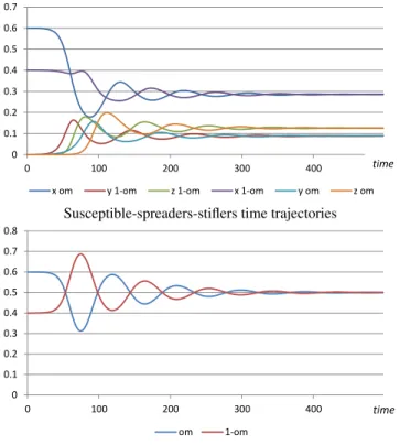
Figures 2 and 3 display illustrative time trajectories for the dynamics of the senti-ment-switching model for specific values of parameters. For the construction of Fi-gure 2, it is assumedλω=λ1−ω=0.25;σω=σ1−ω=1/3;θω=θ1−ω=0.05. The

upper panel presents the time trajectories of the six categories of agents; as one ob-serves, the values of variables oscillate around the steady-state as they approach it. Furthermore, compared with Figure 1, it is evident that the number of spreaders, for each class of sentiment, never falls to zero; as spreaders become stiflers, some previ-ously susceptible individuals become spreaders. This dynamic process is possible be-cause the susceptible category continuously receives individuals that no longer spread the respective sentiment. Note, as well, that, according to the result in Proposition 2, values ofx∗,y∗andz∗are identical for both sentiments. The lower panel represents

(10)

Sentiment Cyclicality

1 Sentiment Cyclicality

Figures

Fig.1: Time trajectories of the shares of susceptible, spreader and stifler individuals (=0.25, = 1/3)

-0.15 0.05 0.25 0.45 0.65 0.85 1.05 0 25 50 75 100 0 0.1 0.2 0.3 0.4 0.5 0.6 0.7 0 100 200 300 400

time

time x

y z

Susceptible-spreaders-stiflers time trajectories

2

Fig.2: Sentiment-switching dynamics (example 1) Lower panel: optimists-pessimists time trajectories

0 0.1 0.2 0.3 0.4 0.5 0.6 0.7 0.8 0 100 200 300 400 om 1-om 0 0.1 0.2 0.3 0.4 0.5 0.6 0.7 0 100 200 300 400

time

Optimists-pessimists time trajectories

Figure 2.Sentiment-switching dynamics (λω=λ1−ω=0.25;σω=σ1−ω=0.33;

θω=θ1−ω=0.05)

the shares of optimists and pessimists; the symmetry triggered by the coincidence in parameter values implies thatω∗=1−ω∗=0.5.

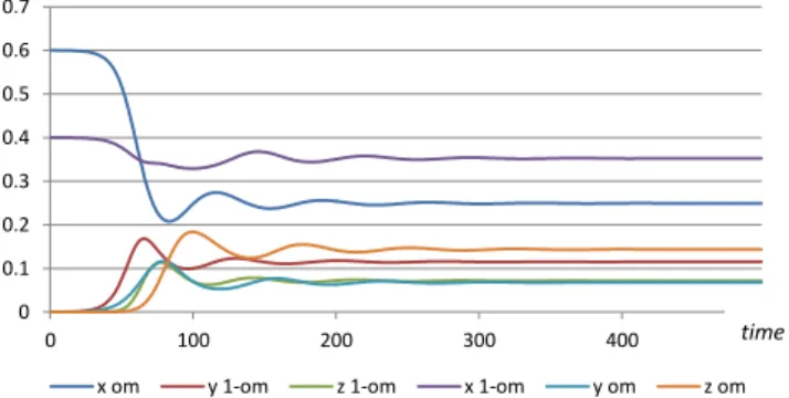
Figure 3 is generated for different parameter values of the various rates under each sentiment. In particular, the example takes λω=0.25; λ1−ω=0.3,σω=1/3;

σ1−ω=0.5;θω=0.05;θ1−ω=0.1. Differences in parameters annulate the

steady-state symmetry and make the number of optimists differ, in the long-run, relatively to the number of pessimists. In this particular case,ω∗=0.46068, 1−ω∗=0.53932.

4. The cyclicality mechanism

Sentiment switching, as characterized in the previous section, generates time series for the shares of optimists and pessimists that exhibit an oscillatory movement. As time unfolds, however, such cycles tend to diminish their intensity and fade away as the val-ues of variables converge to their steady-state positions. In this section, we introduce an additional assumption, which allows for the cyclical motion of the sentiment shares to be perpetuated in time.

(11)

O. Gomes

2

0 0.1 0.2 0.3 0.4 0.5 0.6 0.7 0.8 0 100 200 300 400 om 1-om 0 0.1 0.2 0.3 0.4 0.5 0.6 0.7 0 100 200 300 400

time

3

Fig.4: Sentiment cycles (example 1)

Upper panel: susceptible-spreaders-stifles time trajectories

0 0.1 0.2 0.3 0.4 0.5 0.6 0.7 0 100 200 300 400 om 1-om 0 0.1 0.2 0.3 0.4 0.5 0.6 0.7 0.8 0 100 200 300 400

time

Optimists-pessimists time trajectories

Figure 3.Sentiment-switching dynamics (λω =0.25; λ1−ω=0.3, σω =0.33; σ1−ω=0.5;

θω=0.05;θ1−ω=0.1)

The new assumption requires maintaining the values of parameters σω, σ1−ω,

θωandθ1−ωconstant, but to allowλωandλ1−ωto take different values in two

differ-ent circumstances. Specifically, we consider that the groups of susceptible agdiffer-ents are able to observe the rates of infection and to separate two cases, the one in which the growth rate of sentiment spreading is non negative and the opposite case. Susceptible agents will react as follows:

(i) If the growth rate at which optimistic/pessimistic sentiments are spread is tive or zero, then the rate at which pessimists/optimists are infected with a posi-tive/negative sentiment is high;

(ii) If the growth rate at which optimistic/pessimistic sentiments are spread is nega-tive, then the rate at which pessimists/optimists are infected with a positive/nega-tive sentiment is low.

This mechanism translates the idea that the strength of sentiment spreading influ-ences how susceptible the susceptible individuals are. They are more susceptible if

(12)

3

0 0.1 0.2 0.3 0.4 0.5 0.6 0.7 0 100 200 300 400 om 1-om 0 0.1 0.2 0.3 0.4 0.5 0.6 0.7 0.8 0 100 200 300 400

time

4

Fig.4: Sentiment cycles (example 1) Lower panel: optimists-pessimists time trajectories

0 0.1 0.2 0.3 0.4 0.5 0.6 0.7 0.8 0 100 200 300 400 om 1-om 0 0.1 0.2 0.3 0.4 0.5 0.6 0.7 0.8 0 100 200 300 400

time

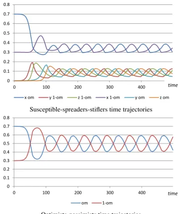
Optimists-pessimists time trajectories Figure 4.Sentiment cycles (λω

0 =λ 1−ω 0 =0.1;λ1ω=λ 1−ω 1 =0.25;σω=σ1−ω=0.33; θω=θ1−ω=0.05 )

the sentiment is propagating at an increasing rate. Analytically, the described process might be formulated in the following form:

λ1−ω,t=  λ₀1−ωifγ_tω₋₁<0 λ₁1−ωifγ_tω₋₁≥0 , γ ω t =  yω t −yωt−1  /yω t−1, λ1 −ω 0 <λ 1−ω 1 and λω,t=  λ₀ωifγ_t1₋−₁ω<0 λ₁ωifγ_t1₋−₁ω≥0 , γ 1−ω t =  y1−ω t −y1 −ω t−1  /y1−ω t−1, λ ω 0 <λ1ω

The reaction of susceptible individuals to the observed spreading rate triggers a perpetual cyclical movement on the shares of ignorants, spreaders and stiflers for both pessimists and optimists and, as a result, the number of optimists and pessimists will

(13)

O. Gomes

4

0 0.1 0.2 0.3 0.4 0.5 0.6 0.7 0.8 0 100 200 300 400 om 1-om 0 0.1 0.2 0.3 0.4 0.5 0.6 0.7 0.8 0 100 200 300 400

time

5

Fig. 6: Output gap time trajectory (g=0) (sentiment propagation example 1)

0 0.1 0.2 0.3 0.4 0.5 0.6 0.7 0.8 0 100 200 300 400 om 1-om -0.01 -0.03 -0.05 0.01 0.03 0.05 0.07 0 100 time time g*

Optimists-pessimists time trajectories Figure 5.Sentiment cycles (λω

0 =λ 1−ω 0 =0.1;λ1ω=0.25;λ 1−ω 1 =0.3;σω=0.33; σ1−ω=0.5;θω=0.05;θ1−ω=0.1 )

be continuously changing. Figures 4 and 5 illustrate this process for the same array of parameter valuesσω,σ1−ω,θωandθ1−ωas the one used to draw Figures 2 and 3. The

only change is in the values ofλ; now, we takeλ₀ω=λ₀1−ω=0.1,λ₁ω=λ₁1−ω=0.25, in the first case, andλ₀ω=λ₀1−ω=0.1,λ₁ω=0.25,λ₁1−ω=0.3 in the second case.

The adaptation of the rumor propagation model to the sentiment-switching process with a cyclicality mechanism exemplifies how sentiments of optimism and pessimism might spread regardless from economic conditions. There are periods in which the ma-jority of the agents adopts an optimistic view of the world just because this sentiment is being propagated faster than the opposite sentiment. Under the proposed process, this situation tends to be reversed after some time periods, making pessimistic feel-ings to dominate in a given time interval; then, optimistic feelfeel-ings take over again as dominant, and this process continues indefinitely.

Now that we have described the mechanism of aggregate mood swings that occur in a context of social interaction, next sections will integrate this behavioral process into a simple macro model.

(14)

Sentiment Cyclicality 5. Optimistic and pessimistic expectations

Sentiments might play a fundamental role on the process of formation of expectations, namely when some kind of departure relatively to the benchmark of rational expecta-tions is considered, i.e., when some sort of bounded rationality is taken into account. Effectively, in order to proceed with the analysis it is now introduced a less than per-fect forecasting rule. At this respect, we follow Brock et al. (2006), Dudek (2010) and Gomes (2012), who consider a device of ’optimized rationality’, according to which the information required to form educated expectations is costly and agents have to weigh the benefits of generating accurate expectations against the cost associated to the acquisition and to the treatment of relevant information.

Agents will be interested in forming expectations about two variables: the inflation rate,πt, and the output gap,gt. Agents ignore, at periodt, the values these variables will take in the subsequent period,t+1, but they can collect information in order to improve the reliability of the expectations. Information acquisition is costly. Each individual may acquire a predictor of a given quality; the better the quality, the more it will cost. When purchasing a predictor of quality qt ∈(0,1), the individual will be acquiring a signalvt. The exact shape of the signal depends on the type of agent, optimistic or pessimistic, one is considering. Specifically, the following signals are available to be acquired:

(i) Signal on future inflation, acquired by an optimistic agent:

vω,π t =  πt+1, with probabilityqωt,π πt−ε(πt−π), with probability 1−qωt,π, ε>0 (4) When acquiring, at periodt, a signalvω,π

t , through the purchase of a predictor of qualityqω,π

t , one of two outcomes is possible: the signal will reveal the true value of the inflation rate with a probabilityqω_t ,π; the same signal will be totally uninformative with a probability 1−qω_t,π. An uninformed agent will make the following forecast for the inflation rate at periodt+1: because the agent is optimistic, she will believe that the inflation rate will converge towards a socially known and accepted target valueπ. This target might be, for instance, the objective set by the central bank to guarantee price stability. Hence, the expectation formed by the optimistic agent regarding future inflation is Eω t  πt+1|vωt ,π  =qω_t,ππt+1+1−qωt ,π  [πt−ε(πt−π)]. (5)

(ii) Signal on future inflation, acquired by a pessimistic agent:

v1_t−ω,π=



πt+1, with probabilityqt1−ω,π

πt+ε(πt−π), with probability 1−qt1−ω,π

(6)

A pessimistic agent, as an optimistic one, will be capable of predicting the true value of the inflation rate with a probability that corresponds directly to the quality of the predictor. However, if the agent is unable to produce the accurate forecast, what

(15)

O. Gomes

occurs with a probability 1−q1t−ω,π, then she will take the pessimistic attitude, which is, in this case, to believe that the inflation rate will diverge from the target value. The same parameterεis considered in (4) and (6) in order to maintain a symmetry between the behavior of optimists and pessimists. In this case, the individual expectation is

E1−ω t  πt+1|v1t−ω,π  =q1_t−ω,ππt+1+  1−q1_t−ω,π[πt+ε(πt−π)]. (7) Signals with a similar structure can be built for the output gap. Letgbe the target defined by public authorities for this aggregate and recognized by the population as such; denote byη the rate at which uninformed agents expect a convergence (if they are optimists) or a divergence (if they are pessimists) relatively to the respective target value.

(iii) Signal on future output gap, acquired by an optimistic agent:

vω_t ,g=



gt+1, with probabilityqωt ,g

gt−η(gt−g), with probability 1−qωt ,g, η>0

(8)

(iv) Signal on future output gap, acquired by a pessimistic agent:

v1_t−ω,g=  gt+1, with probabilityq1t−ω,g gt+η(gt−g), with probability 1−q1 −ω,g t (9)

The respective expectations are: Eω t  gt+1|vtω,g  =qω_t ,ggt+1+  1−qω_t ,g[gt−η(gt−g)] (10) E1−ω t  gt+1|v1 −ω,g t  =q1_t−ω,ggt+1+  1−q1_t−ω,g[gt+η(gt−g)] (11) Next, we must approach how probabilities reflecting the quality of the signal are determined. At each datet, agents intend to purchase an optimal predictor, i.e., a predictor that delivers the best possible balance between the accuracy of the forecast and the minimization of information acquisition and processing costs. In this case, optimists and pessimists will, respectively, solve the following optimality problems:

min qω,πt ,q ω,g t Uω t = 1 2  Eω t  πt+1|vωt ,π  −πt+12+ (12) +1 2a  Eω t  gt+1|vtω,g  −gt+12+Cqtω,π,q ω,g t  , and min q1_t−ω,π,q1_t−ω,g U1−ω t = 1 2  E1−ω t  πt+1|v1t−ω,π  −πt+1 2 + (13) +1 2a  E1−ω t  gt+1|v1t−ω,g  −gt+1 2 +Cq1−ω,π t ,q1 −ω,g t 

(16)

Sentiment Cyclicality In (12) and (13), parametera>0 represents the weight given to output stabilization relatively to price stability in the agents’ objective functions, and functionsC(·) trans-late the costs of acquisition of each one of the predictors. Convex cost functions are taken: C(q_tω,π,qω_t ,g) =1 2ψ _ q_tω,π2+q_tω,g2, ψ≥0 (14) C(q1−ω,π t ,q1 −ω,g t ) = 1 2ψ _ q1−ω,π t 2 +q1_t−ω,g2  (15) The solutions of problems (12) and (13) are:

∂U_tω ∂qωt,π =0 ⇔ qω,π t = [πt+1−πt+ε(πt−π)]2 ψ+ [πt+1−πt+ε(πt−π)]2 (16) ∂Ut1−ω ∂qt1−ω,π =0 ⇔ q1_t−ω,π= [πt+1−πt−ε(πt−π)] 2 ψ+ [πt+1−πt−ε(πt−π)]2 (17) ∂Uω t ∂qωt ,g =0 ⇔ qω_t,g= a[gt+1−gt+η(gt−g)] 2 ψ+a[gt+1−gt+η(gt−g)]2 (18) ∂U1−ω t ∂q1t−ω,g =0 ⇔ q1_t−ω,g= a[gt+1−gt−η(gt−g)] 2 ψ+a[gt+1−gt−η(gt−g)]2 (19)

Optimal predictors (16) to (19) reflect the importance of information acquisition costs in forming expectations. Costless information (ψ =0) impliesq=1 for every predictor, meaning that perfect foresight prevails. As the value of the cost parameter increases, the quality of the signal will fall and the perfect foresight outcome becomes progressively less probable. Although it is possible to compute optimal predictors, as presented above, these depend on future values of the inflation rate and of the output gap that are not known at datet(the predictors are used precisely because such values are not known with anticipation!). To circumvent this obstacle, various approaches are possible; Brock et al. (2006), for instance, resort to the concept of managerial perfect foresight equilibrium, while Dudek (2010) considers the possibility of computing an average of all the available signals. The approach we follow is simpler; it is considered that agents know the perfect foresight steady-state(π_,g_)and, in order to save effort and cognitive resources, they adopt a constant in time predictor where observable values of variables give place to the perfect foresight steady-state values. The inflation rate and the output gap(π_,g_)depend on the specific macro structure of the economy.2 For an economy that is hypothetically resting in the defined steady-state, predictors (16) and (17) are identical,  qω,π₌  q1−ω,π₌ [ε(π−π)] 2 ψ+ [ε(π−π)] 2, (20)

2 _{These values are presented, in explicit form, in the next section, for the New-Keynesian model.}

(17)

O. Gomes  qω,g₌  q1−ω,g₌ a[η(g−g)] 2 ψ+a[η(g_−g)]2. (21)

Reconsider now expectations (5), (7), (10) and (11). By replacing the predictor values (16) and (17) in them, one obtains explicit expressions for each of the relevant expectations, Eω t  πt+1|vtω,π  =[ε(π−π)] 2 πt+1+ψ[πt−ε(πt−π)] ψ+ [ε(π−π)] 2 , (22) E1−ω t  πt+1|vt1−ω,π  =[ε(π−π)] 2 πt+1+ψ[πt+ε(πt−π)] ψ+ [ε(π−π)] 2 , (23) Eω t  gt+1|vωt,g  =a[η(g−g)] 2 gt+1+ψ[gt−η(gt−g)] ψ+a[η(g_−g)]2 , (24) E1−ω t  gt+1|v1 −ω,g t  =a[η(g−g)] 2 gt+1+ψ[gt+η(gt−g)] ψ+a[η(g_−g)]2 . (25)

Observe, for expectations (22) to (25), that the absence of information costs implies a return to perfect foresight, i.e.,ψ=0⇒Etω

 πt+1|vtω,π  =E1−ω t  πt+1|v1 −ω,π t  =πt+1 andEω t  gt+1|vωt ,g  =E1−ω t  gt+1|v1t−ω,g  =gt+1.

Since we are interested in dealing with aggregate expectations, we have to com-pute the weighted average expectations in the economy. Given the shares of optimists and pessimists that populate the economy at datet, computed according to what was established in Section 4, such expectations are

Et(πt+1) =ωtE_tωπt+1|vωt,π  + (1−ωt)E_t1−ω  πt+1|v1t−ω,π  , (26) Et(gt+1) =ωtEtω  gt+1|vωt ,g  + (1−ωt)E1−ω t  gt+1|vt1−ω,g  . (27)

The final expressions of the inflation rate and of the output gap expectations are obtained by replacing (22) and (23) into (26), and (24) and (25) into (27). They are,

Et(πt+1) = [ε(π−π)] 2 πt+1+ψ[πt+ε(1−2ωt)(πt−π)] ψ+ [ε(π−π)] 2 , (28) Et(gt+1) = a[η(g−g)] 2_g t+1+ψ[gt+η(1−2ωt)(gt−g)] ψ+a[η(g_−g)]2 . (29)

Note, also on the aggregate level, that ifψ=0, thenEt(πt+1) =πt+1andEt(gt+1) =

gt+1.

(18)

Sentiment Cyclicality 6. Application to the New-Keynesian macro model

In this section, a characterization of the long-term dynamics of the New-Keynesian model is undertaken, taking into account expectation formation rules (28) and (29). We consider a reduced form of the model, which contemplates two difference equations, describing the demand-side and the supply-side of the economy.3 The two equations are a dynamic IS curve that establishes the common opposite sign relation between the real interest rate,rt, and the output gap,

gt=−ϕrt+Et(gt+1) +µt, ϕ>0, (30) and a New-Keynesian Phillips curve,

πt=κgt+βEt(πt+1) +υt, κ,β ∈(0,1). (31) Parameterβ is the discount factor andκ measures the degree of price stickiness; the lower the value ofκ, the stickier prices are. Variablesµt andυt correspond to white noise disturbances that influence, respectively, demand and supply. The real interest rate is given by the Fisher equation,rt=it−Et(πt+1), withitthe nominal interest rate;

and monetary policy is implemented through a standard Taylor rule,

it=ρit−1+ (1−ρ)φπ[Et(πt+1)−π] +φggt, ρ∈(0,1),φπ>1,φg≥0. (32)

In equation (32), parameterρ translates policy inertia. Valuesφπ andφgare

po-licy parameters. Conditionφπ >1 guarantees, under this model’s specification, the

determinacy of the model,∀φg≥0.

Our goal is not to pursue a thorough investigation of the model’s dynamics; in-stead, we will concentrate the analysis in the steady-state. First, we derive the perfect foresight steady-state equilibrium.

Proposition 3. A perfect foresight steady-state equilibrium for the New-Keynesian macro model composed by equations (30), (31) and (32) exists, it is unique and it is given by the pair of values

(π,g) =  φπ φπ−1+ 1−β κ φg π; _κ φπ 1−β(φπ−1) +φg π  .

Proof. Solve the system (30)–(32) under conditionsπ_≡πt =Et(πt+1), g≡gt =

Et(gt+1),µt=υt=0.

Observe that, as long as the target inflation rate is positive, the values ofπ_andg will also be positive, given the conditionφπ >1. If the central bank aims at a zero

inflation rate, the perfect foresight equilibrium implies that not only the inflation rate but also the output gap are equal to zero. The system of equations allows, as well, to determine the steady-state value of the nominal interest rate, under conditions of

3 _{See Clarida et al. (1999) and Woodford (2003), for details on the New-Keynesian model.}

(19)

O. Gomes

perfect foresight, which isi=π; i.e., in the perfect foresight equilibrium, the real interest rate is equal to zero.

Next, we need to compute the steady-state not under perfect foresight but under the sentiment expectations derived in the previous section. As in De Grauwe (2011) we re-mark that the microfoundations of this model were built under the implicit assumption that the expectations are rational and that one should be careful when extrapolating the analysis of the reduced form of the model to a scenario of bounded rationality; as in the mentioned paper, we follow the arguments in Evans and Honkapohja (2001), in order to consider it an admissible assumption. We define(π∗,g∗)as the steady-state that will hold under the following long-term expectations,

Et(π∗) =π∗+ (1−2ωt) ψ ε(π∗−π) ψ+ [ε(π−π)] 2, (33) Et(g∗) =g∗+ (1−2ωt) ψ η(g ∗₋_g₎ ψ+a[η(g_−g)]2 . (34)

Expectations (33) and (34) are steady-state expectation values withdrawn from (28) and (29) under conditionsπ∗≡πt+1=πtandg∗≡gt+1=gt. These long-run expecta-tions have interesting features. Expectaexpecta-tions will coincide with observed steady-state values (what implies long-term perfect foresight) in four possible scenarios: (i) absence of information costs (ψ=0); (ii) neutral sentiments (ε=0;η=0); (iii) coincidence between target values and steady-state levels (π∗=π;g∗=g); (iv) identical number of pessimists and optimists (ωt=1/2). In the above expectations, we maintain the time subscript because shareωtis subject, under the assumption introduced in Section 4, to perpetual motion.

Proposition 4. The steady-state equilibrium under sentiment cyclicality exists, it is unique and it is the pair of values

 π∗ g∗  =      ϕ[(φπ−1)Θt+φπ] + (Λt−ϕ φg)βκΘt  π−Λtg ϕ(φπ−1)(1+Θt) + (ϕ φg−Λt)_κ1[1−β(1+Θt)] 1 κ[1−β(1+Θt)]π ∗₊β κΘtπ     withΘt≡(1−2ωt) ψ ε ψ+[ε(π−π)] 2 andΛt≡(1−2ωt) ψ η ψ+a[η(g−g)] 2.

Proof. Solve the system (30)–(32) under conditionsπ∗≡πt=πt+1,g∗≡gt=gt+1,

µt=υt=0, and with expectations given by (33) and (34). UnderΘt=Λt=0, we confirm that(π∗,g∗) = (π,g).

The comparison between the two steady-state results highlights essentially that cyclical sentiments can transform an otherwise fixed-point steady-state into a regu-lar fluctuations long-term scenario. However, our setup is not fully deterministic and we might consider that demand and supply shocks continue to hit the economy in the long-run. In what follows, we numerically simulate the long-term outcome, compar-ing the rational expectations setup with the one that assumes sentiments. For such, we

(20)

Sentiment Cyclicality rewrite the steady-state results without the removal of the exogenous disturbances. We have:

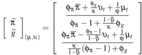
(i) Rational expectations long-run outcome,

  π  g  (µ,υ) =       φππ+ φg κυt+ 1 ϕµt φπ−1+ 1−β κ φg φππ− φπ−1 1−β υt+ 1 ϕµt κ 1−β(φπ−1) +φg      

(ii) Sentiment expectations long-run outcome,   π  g  (µ,υ) =    ϕ[(φπ−1)Θt+φπ]+(Λt−ϕ φg)β_κΘt  π−Λtg+(ϕ φg−Λt)_κ1υt+µt ϕ(φπ−1)(1+Θt)+(ϕ φg−Λt)_κ1[1−β(1+Θt)] 1 κ[1−β(1+Θt)]π ∗₊β κΘtπ− 1 κυt  

The nature of the shocks is straightforward to understand from the rational expecta-tions case: positive cost-push shocks rise inflation and lower output; positive demand shocks rise inflation and make effective output to increase as well, relatively to the potential level. In order to address business cycles dynamics, we will concentrate the analysis on the output gap series. Under rational expectations, the only source of fluctuations is the random realizations of the disturbance variables; in the sentiment scenario, an additional source emerges: sentiment cyclicality. The example that fol-lows alfol-lows to illustrate how waves of optimism and pessimism imply a change on the interpretation one can make about long-term fluctuations.

The parameter values selected for the analysis are displayed in Table 1. Those which have to do directly with the macro model specification (the first row of values) are withdrawn from Woodford (2003, p. 341, 285); the others are reasonable and plau-sible values, that do not interfere significantly with the qualitative nature of the results.

Table 1.Parameter values

β=0.99;ϕ=6.25;κ=0.024;φπ=2;

π=0.02;g=0.01;ψ=1;ε=0.175;η=0.2;a=0.25 µt∼N(0; 2.5×10−7);υt∼N(0; 2.5×10−7)

There is a parameter missing in Table 1. It is the monetary policy parameter asso-ciated with real stabilization. This is because the parameter has an important role in determining the results to be obtained and, therefore, to illustrate its relevance we will work with three different values:φg=0,φg=0.25 andφg=0.5.

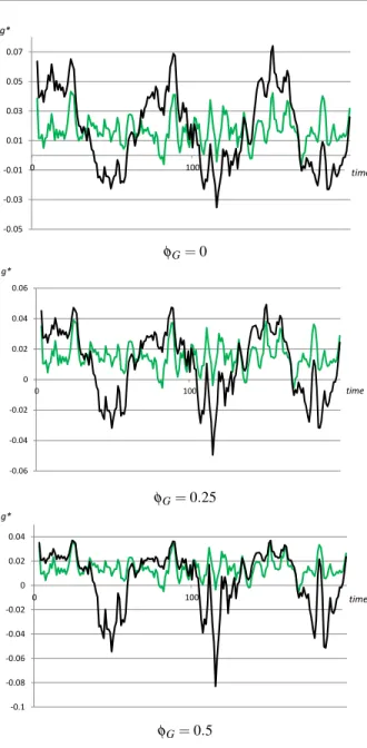
Figures 6 and 7 display the long-term trajectories of the output gap, comparing the rational expectations and the sentiment cycles outcomes. Each figure corresponds to each one of the cases depicted in Figures 4 and 5 (recall that the difference between the

(21)

O. Gomes

5

Fig. 6: Output gap time trajectory (g=0)

(sentiment propagation example 1)

0 0.1 0.2 0.3 0.4 0.5 0.6 0.7 0.8 0 100 200 300 400 om 1-om -0.01 -0.03 -0.05 0.01 0.03 0.05 0.07 0 100 time time g* φG=0 6

Fig. 6: Output gap time trajectory (g =0.25)

Fig.6: Output gap time trajectory (g =0.5)

(sentiment propagation example 1) -0.02 -0.04 -0.06 0 0.02 0.04 0.06 0 100 -0.02 -0.04 -0.06 -0.08 -0.1 0 0.02 0.04 0 100 time g* time g* φG=0.25 6

Fig. 6: Output gap time trajectory (g =0.25)

-0.02 -0.04 -0.06 0 0.02 0.04 0.06 0 100 -0.02 -0.04 -0.06 -0.08 -0.1 0 0.02 0.04 0 100 time g* time g* φG=0.5

Figure 6.Output gap time trajectory: sentiment propagation example 1

two has to do with the values of parameters in the susceptible-spreader-stifler frame-work). Each figure has three panels that represent, from up to bottom, the casesφg=0, φg=0.25 andφg=0.5. In each figure, 200 time periods are assumed. In order to smooth the fluctuations, the presented trajectories are displayed as trend lines over the

(22)

7

Fig.7: Output gap time trajectory (g=0)

-0.01 -0.03 -0.05 0.01 0.03 0.05 0 100 -0.01 -0.03 -0.05 -0.07 0.01 0.03 0.05 0 100 time g* time g* φG=0 7

Fig.7: Output gap time trajectory (g=0)

-0.01 -0.03 -0.05 0.01 0.03 0.05 0 100 -0.01 -0.03 -0.05 -0.07 0.01 0.03 0.05 0 100 time g* time g* φG=0.25 8

Fig.7: Output gap time trajectory (g =0.5) (sentiment propagation example 2)

Fig. 8: Utility of the central bank for different policy parameter values.

-0.2 -0.15 -0.1 -0.05 0 0 100 -8 -7 -6 -5 -4 -3 -2 -1 0 -0.1 6E-16 0.1 0.2 0.3 0.4 0.5 0.6 time g* =2.05 < L > g =2 =1.95 φG=0.5

Figure 7.Output gap time trajectory: sentiment propagation example 2

original time-series taking a 4-period moving average. The darker lines correspond to the trajectories of the output gap under sentiment cyclicality; the brighter ones corre-spond to the rational expectations outcome.

Both figures show an evident result: the way sentiment cyclicality impacts on

(23)

O. Gomes

gregate fluctuations is strongly influenced by the value of parameterφg. Time trajec-tories in Figure 6 differ from the ones in Figure 7 for just one fundamental reason: the number of pessimists is, on average, larger than the number of optimists in the case of Figure 7 and, thus, the output gap is, on average, a lower value on each of the three dis-played examples. Concentrating the attention on the trajectories provided by Figure 6, note the following; when monetary authorities show no concern with real stabilization, sentiment cycles exacerbate both periods of expansion and periods of contraction of the economy, relatively to the benchmark of rational expectations. This introduces a more pronounced cyclical movement on a time series that otherwise follows a relatively er-ratic behavior. As we increase the value of φg, a relevant phenomenon occurs: the introduction of waves of optimism and pessimism do not generate periods of remark-able expansions relatively to the case of rational expectations; however, it allows for the occurrence of strong recessions, in which the trajectory of the output gap departs significantly from what the rational expectations analysis would predict.

Therefore, through the inspection of the trajectories, we find both a source of strong recessions and a policy recommendation to avoid them: strong recessions are the result of a an output stabilization effort on the part of the central bank; in order to avoid them, monetary authorities should concentrate on the price stability goal.4

Synthesizing, cycles of large amplitude are the result of a series of events that, once combined, can lead to strong recessions; they are:

(i) The social interaction process that transforms optimists into pessimists and the opposite, in a recurrent way over time;

(ii) Information costs, that prevent individuals from gaining access, under optimal conditions, to the knowledge required to formulate rational expectations; (iii) Price stickiness, which is the main foundation on which the New-Keynesian

model and, in particular, the New-Keynesian Phillips curve is built upon; (iv) A misdirected monetary policy effort, that puts too much weight on output

sta-bilization.

To gain further insights on the role of waves of optimism and pessimism over the benchmark New-Keynesian macro model, let us now simultaneously consider both policy goals: price stability and real stabilization. The following monetary policy objective function is adapted from Geraats (1999),

Lt=− 1 2[(π ∗ t −π)×100] 2₊_{b f}₍₍_g∗ t −g)×100). (35)

4 _{In de Grauwe (2011), it is suggested that the presence of animal spirits will imply that inflation targeting} monetary policy may no longer be optimal and that output stabilization could in fact improve welfare. An-geletos and La’O (2013) present arguments in the opposite direction: strategic uncertainty coming from an-imal spirits will contribute to an ineffective policy and, thus, the monetary authority should refrain pursuing measures that go beyond its main assignment, which is to guarantee price stability. The second interpretation is closer to the line of reasoning and to the results in this paper.

(24)

Sentiment Cyclicality In expression (35),π_t∗andg∗_t furnish long-term values for inflation and output gap in the sentiment case; their time series are the ones displayed in Figure 6.5 _Parameter

b≥0 reflects the weight of output stabilization as a policy goal, relatively to the price stability objective. Function fis such that f00<0 and f000>0, what signifies that nega-tive deviations from the output gap target are more penalized than posinega-tive deviations, from the point of view of the central bank’s objective. This is the same as saying that the central bank has a strong dislike for recessions. An admissible functional form, which obeys to the specified conditions, is

f((g∗_t −g)×100) =1−exp  −1 2(g ∗ t−g)×100  −1 2(g ∗ t −g)×100. (36) Note that f(0) =0, i.e., when the value of the output gap coincides with the target, then the contribution of the output gap to the objective valueLt is zero. Observe, as well, that f <0 forg∗_t 6=g, i.e., f(0)is the maximum value of f.

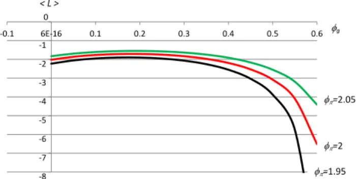
Given objective function (35) and the previously assumed parameter values, to which we addb=0.048 (Woodford 2003, p. 431), one can make an inspection about the role that both policy parameters,φπandφg, have in allowing for a desirable policy

result. Figure 8 draws the relation between the value of parameterφgand an average of the value of Lover 200 long-term periods, hL200i. Three lines are displayed, for

different values of the other parameter,φπ=1.95,φπ =2,φπ=2.05. The results are

evident: in order to maximize its utility, the central bank will have to choose between policies according to the following requisites,

(i) The larger the value ofφπ, i.e., the more aggressive monetary policy is in terms

of promoting price stability, the higher is the obtained utility;

(ii) Real stabilization policy measures may enhance the utility outcome if it is ap-plied with moderation. The figure indicates that, for each value ofφπ, the value

ofφgthat maximizes the average value ofLis located aroundφg=0.2.

Therefore, for a central bank that has, as policy goals, price stability and the avoid-ance of strong recessions, the effectiveness of its policy is best achieved by adopting an aggressive attitude relatively to price stability and by addressing, as well, output gap stabilization concerns, although changes in the interest rate to respond to output gap fluctuations should be relatively moderate.

Finally, we compare, for a specific policy valueφπ =2, the relation between φg

andhLiunder sentiment cycles and rational expectations. It is evident that the less intense fluctuations of the rational expectations case generate a better fit relatively to the designed policy goals, as shown in Figure 9. Thus, prior to specific policy actions, authorities should address another challenge: how can animal spirits be attenuated. If animal spirits refer, as pointed out in the introduction, to confidence, fairness and social attitudes, society should direct its efforts to promote ethical principles and education in

5 _{The analysis is now restricted to a single case, namely the one in which identical parameter values for the} sentiment switching setup are assumed.

(25)

O. Gomes

8

Fig.7: Output gap time trajectory (g=0.5) (sentiment propagation example 2)

Fig. 8: Utility of the central bank for different policy parameter values. -0.2 -0.15 -0.1 -0.05 0 0 100 -8 -7 -6 -5 -4 -3 -2 -1 0 -0.1 6E-16 0.1 0.2 0.3 0.4 0.5 0.6 time g* =2.05 < L > g =2 =1.95

Figure 8.Utility of the central bank for different policy parameter values

9

Fig.9: Utility of the central bank – comparison between rational expectations and sentiment cycles. -0.5 -1 -1.5 -2 -2.5 -3 -3.5 -4 -4.5 -5 0 0 0.2 0.4 0.6 0.8 1 < L > g RE SC

Figure 9.Utility of the central bank - comparison between rational expectations and sentiment cycles

order to attenuate the intensity of the sentiment switching that underlies the observed fluctuations on economic aggregates.

7. Conclusion

This paper proposed a foundation for the persistence of fluctuations in the aggregate sentiment level. Waves of optimism and pessimism alternate as the result of a fully deterministic dynamic process in which pessimists become optimists and optimists become pessimists under a susceptible-spreader-stifler sequence.

The cyclical nature of animal spirits, as discussed, can be introduced into a typical macroeconomic model in order to justify, at least partially, observed business cycles. The compatibility between the sentiment framework and a description of the macro environment requires some sort of departure relatively to the rational expectations paradigm. In this specific case, we consider a setting where the information required to

(26)

Sentiment Cyclicality form accurate predictions about future events is costly and, thus, agents’ expectations may deviate from perfect foresight; when this occurs, agents will be optimistic or pes-simistic about the future performance of the economy, with the shares of optimists and pessimists determined by the characterized rumor propagation framework.

The setup suggests that, in the long-term, observed fluctuations are strongly de-termined by sentiment switching with origins in social interaction. In this sense, the study supports the Keynesian view on animal spirits, that interprets business cycles as the outcome of forces that have to do with mass psychology much more than with con-crete economic phenomena. Business cycles are the result of uncontrollable behavioral factors, and there is not much public authorities can do to avoid cyclical movements in sentiments, except contributing to a society based on fairness, confidence and social collaboration and cohesion.

However, the same is not true in what concerns the way sentiments shape expec-tations and impact on macro variables. Adequate policies to reduce the effect of sys-tematic sentiment changes over the performance of the economy are essentially those that (i) reduce the cost of information acquisition; (ii) establish reasonable and realistic policy targets; (iii) develop monetary policy measures, by manipulating policy parame-ters, that might fight the undesirable consequences of natural sentiment fluctuations.

The analysis also suggested that, in the context of the New-Keynesian model, a strong effort to stabilize output may be counterproductive and may generate or perpet-uate strong recessions. This conclusion is in syntony with a neoclassical interpretation of monetary policy intervention (i.e., the central bank should concentrate exclusively on its price stability mandate and avoid real stabilization measures that are often inef-fective), what places the analysis in this paper in a same class as Angeletos and La’O (2013): although a Keynesian cornerstone is added to the discussion, the implications of the analysis are typically neoclassical, with observed cycles being largely deter-mined by uncontrollable sentiment fluctuations that are due to interaction and com-munication frictions that cannot be successfully mitigated through direct stabilization policy intervention.

Acknowledgement I would like to acknowledge the helpful comments of two anony-mous referees. The usual disclaimer applies.

References

Akerlof, G. A. and Shiller, R. J. (2009). Animal Spirits: How Human Psychology Drives the Economy, and Why It Matters for Global Capitalism. Princeton, NJ: Prince-ton University Press.

Angeletos, G. M., Collard, F. and Dellas, H. (2015). Quantifying Confidence. DO-PLNITCEPR discussion papersNo. 10463.

Angeletos, G. M. and La’O, J. (2013). Sentiments.Econometrica, 81, 739–779. Bidder, R. M. and Smith, M. E. (2012). Robust Animal Spirits. Journal of Monetary Economics, 59, 738–750.

(27)

O. Gomes

Bofinger, P., Debes, S.,Gareis, J. and Mayer, E. (2013). Monetary Policy Transmis-sion in a Model with Animal Spirits and House Price Booms and Busts. Journal of Economic Dynamics and Control,37, 2862–2881.

Brock, W. A., Dindo, P. and Hommes, C. H. (2006). Adaptive Rational Equilibrium with Forward Looking Agents. International Journal of Economic Theory, 2, 241–278.

Cintron-Arias, A. (2006).Modeling and Parameter Estimation of Contact Processes. Cornell University, Dissertation Thesis.

Clarida, R., Gali, J. and Gertler, M. (1999). The Science of Monetary Policy: A New Keynesian Perspective.Journal of Economic Literature, 37, 1661–1707.

Daley, D. J. and Kendall, D. G. (1964). Epidemics and Rumors.Nature, 204, 1118. Daley, D. J. and Kendall, D. G. (1965). Stochastic Rumours.Journal of the Institute of Mathematics and Its Applications, 1, 42–55.

De Grauwe, P. (2011). Animal Spirits and Monetary Policy. Economic Theory, 47, 423–457.

De Grauwe, P. (2012). Booms and Busts in Economic Activity: A Behavioral Expla-nation.Journal of Economic Behavior and Organization, 83, 484–501.

Dudek, M. K. (2010). A Consistent Route to Randomness. Journal of Economic The-ory, 145, 354–381.

Evans, G. and Honkapohja, S. (2001).Learning and Expectations in Macroeconomics. Princeton, NJ: Princeton University Press.

Franke, R. (2012). Microfounded Animal Spirits in the New Macroeconomic Consen-sus.Studies in Nonlinear Dynamics and Econometrics, 16, 1–41.

Geraats, P. M. (1999). Inflation and Its Variation: An Alternative Explanation. UC Berkeley, Center for International and Development Economics Research, Working Paper No. qt56b2g3vn.

Gomes, O. (2012). Rational Thinking under Costly Information – Macroeconomic Implications.Economics Letters, 115, 427–430.

Huo, L., Huang, P. and Guo, C. X. (2012). Analyzing the Dynamics of a Rumor Trans-mission Model with Incubation. Discrete Dynamics in Nature and Society, article ID 328151.

Kocherlakota, N. R. (2010). Modern Macroeconomic Models as Tools for Economic Policy. Federal Reserve Bank of Minneapolis,the Region, May, 5–21.

Lengnick, M. and Wohltmann, H.-W. (2013). Agent-Based Financial Markets and New Keynesian Macroeconomics: A Synthesis.Journal of Economic Interaction and Coordination, 8, 1–32.

Maki, D. P. and Thompson, M. (1973). Mathematical Models and Applications, with Emphasis on Social, Life, and Management Sciences. Englewood Cliffs, NJ: Prentice-Hall.

(28)

Sentiment Cyclicality Milani, F. (2011). Expectation Shocks and Learning as Drivers of the Business Cycle. Economic Journal, 121, 379–401.

Nekovee, M., Moreno, Y., Bianconi, G. and Marsili, M. (2007). Theory of Rumor Spreading in Complex Social Networks.Physica A, 374, 457–470.

Pastor-Santorras, R. and Vespignani, A. (2004). Evolution and Structure of the Inter-net: a Statistical Physics Approach. Cambridge, UK: Cambridge University Press. Piqueira, J. R. C. (2010). Rumor Propagation Model: An Equilibrium Study. Mathe-matical Problems in Engineering,article ID 631357.

Thompson, K., Estrada, R. C., Daugherty, D. and Cintron-Arias, A. (2003). A De-terministic Approach to the Spread of Rumors. Cornell University, Department of Biological Statistics & Computational Biology, Technical Report BU-1642-M. Wang, Y. Q., Yang, X. Y., Han, Y. L. and Wang, X. A. (2013). Rumor Spreading Model with Trust Mechanism in Complex Social Networks. Communications in Theoretical Physics, 59, 510–516.

Woodford, M. (2003). Interest and Prices: Foundations of a Theory of Monetary Policy. Princeton, NJ: Princeton University Press.

Zanette, D. H. (2002). Dynamics of Rumor Propagation on Small-World Networks. Physical Review E, 65, 041908.

Zhao, L. J., Wang, J. J., Chen, Y. C., Wang, Q., Cheng, J. J. and Cui, H. X. (2012). SIHR Rumor Spreading Model in Social Networks.Physica A, 391, 2444–2453.

(29)

O. Gomes Appendix

Proof of Proposition 1

Applying equilibrium conditionv∗−V(v∗) =0 to system (3), the following chain of equalities will hold in the steady-state,6

θω(z ω₎∗ ₌ λω(x ω₎∗ y1−ω∗ =σω  y1−ω∗ y1−ω∗ +z1−ω∗ (37) = θ1−ω  z1−ω∗ =λ1−ω  x1−ω∗ (yω₎∗₌ σ1−ω(y ω₎∗ (yω₎∗_{+ (}_zω₎∗

From (37), it is straightforward the computation of the following equilibrium rela-tions, (zω₎∗ (z1−ω₎∗ = θ1−ω θω (38) (zω₎∗₌ σ1−ω  (yω₎∗2 θω−σ1−ω(yω) ∗ (39)  z1−ω∗ = σω  y1−ω∗2 θ1−ω−σω(y1−ω) ∗ (40) (xω₎∗₌σω λω _ y1−ω∗ +z1−ω∗ (41)  x1−ω∗ =σ1−ω λ1−ω  (yω₎∗_{+ (}_zω₎∗ (42)

Solving (39) and (40) with respect to(yω₎∗_and y1−ω∗

, respectively, replacing the results into (41) and (42), and making use of relation (38), one can display steady-state values (yω₎∗_,

y1−ω∗

,(xω₎∗_and x1−ω∗

as depending solely on (zω₎∗_{. The}

expressions are: (yω₎∗₌    1+ 4θω σ1−ω(zω) ∗−1 2  (zω) ∗ (43)  y1−ω∗ = θω θ1−ω      1+ 4(θ1−ω) 2 σωθω(zω) ∗−1 2     (zω₎∗ ₍₄₄₎ 6 _Condition_yω 0 6=0∨y 1−ω 0 6=0 is implicitly assumed.