Copyright © UNU-WIDER 2007 1
Department of Economics, University of Western Ontario; 2UNU-WIDER, Helsinki; 3Department of Economics, New York University.
This study has been prepared within the UNU-WIDER project on Personal Assets from a Global Perspective, directed by James B. Davies.
UNU-WIDER acknowledges with thanks the financial contributions to its research programme by the governments of Denmark (Royal Ministry of Foreign Affairs), Finland (Ministry for Foreign Affairs), Norway (Royal Ministry of Foreign Affairs), Sweden (Swedish International Development Cooperation Agency—Sida) and the United Kingdom (Department for International Development).
ISSN 1810-2611 ISBN 978-92-9230-030-2
Research Paper No. 2007/77
Estimating the Level and Distribution
of Global Household Wealth
James B. Davies,
1Susanna Sandström,
2Anthony Shorrocks,
2and Edward N. Wolff
3November 2007 Abstract
We provide the first estimate of the level and distribution of global household wealth. Mean assets and debts within countries are measured, partly or wholly, for 38 countries using household balance sheet and survey data centred on the year 2000. Determinants of mean financial assets, non-financial assets, and liabilities are studied empirically, and the results are used to impute values to countries lacking wealth data. Household wealth per adult is US$43,494 in PPP terms, and ranges regionally from US$11,655 in Africa to US$193,147 in North America. Data on the shape of the household distribution of wealth for 20 countries, accounting for 59 per cent of the world’s population and, we estimate, 84 per cent of its wealth are used to establish patterns of wealth inequality within countries. Imputations are again performed for countries lacking wealth data, on the basis of the observed relation between wealth and income distribution for the 20 countries with data. The Gini coefficient for the global distribution of wealth is 0.804, and the share of the top 10 per cent is 71 per cent. Wealth of US$8,325 is needed to be in the top half of the distribution, and US$517,601 is needed to be in the top one per cent. Between-country differences in wealth are two-thirds of global inequality according to the Gini coefficient, indicating a larger role for within-country inequality than in the case of income according to recent estimates. Keywords: wealth, net worth, personal assets, inequality, households, balance sheets, portfolios
The World Institute for Development Economics Research (WIDER) was established by the United Nations University (UNU) as its first research and training centre and started work in Helsinki, Finland in 1985. The Institute undertakes applied research and policy analysis on structural changes affecting the developing and transitional economies, provides a forum for the advocacy of policies leading to robust, equitable and environmentally sustainable growth, and promotes capacity strengthening and training in the field of economic and social policy making. Work is carried out by staff researchers and visiting scholars in Helsinki and through networks of collaborating scholars and institutions around the world.
www.wider.unu.edu [email protected]
UNU World Institute for Development Economics Research (UNU-WIDER) Katajanokanlaituri 6 B, 00160 Helsinki, Finland
Typescript prepared by Lorraine Telfer-Taivainen at UNU-WIDER
The views expressed in this publication are those of the author(s). Publication does not imply endorsement by the Institute or the United Nations University, nor by the programme/project sponsors, of any of the views expressed.
Acknowledgements
We thank participants at the May 2006 UNU-WIDER project meeting on Personal Assets from a Global Perspective, and the August 2006 International Association for Research in Income and Wealth 29th General Conference in Joensuu, Finland, for their valuable comments and suggestions. Special thanks are due to Tony Atkinson, Brian Bucks, Markus Jäntti, and Branko Milanovic. Responsibility for errors and omissions is our own.
1 Introduction
Much attention has recently been given to estimates of the world distribution of income (Bourguignon and Morrison 2002; Milanovic 2002, 2005). The results show that global income distribution is very unequal and that inequality has not been falling over time. Indeed, in some regions both poverty and income inequality have risen. Interest naturally turns to global inequalities in other dimensions of economic status, resources or wellbeing, of which one of the most important is household wealth.
In everyday conversation the term ‘wealth’ often signifies little more than ‘money income’. On other occasions economists interpret the term broadly and define wealth to be the value of all household resources, both human and non-human. Here, the term is used in its long-established sense of net worth: the value of physical and financial assets less liabilities.1 Wealth in this respect represents the ownership of capital. While only one part of personal resources, capital is widely believed to have a disproportionate impact on household wellbeing and economic success, and more broadly on economic development and growth.
Wealth has been studied carefully at the national level since the late nineteenth or early twentieth century in a small number of countries, for example Sweden, the UK and the USA. In some other countries, for example Canada, it has been studied systematically since the 1950s. And in recent years the number of countries with wealth data has risen fairly quickly. The largest and most prosperous OECD countries all have wealth data based on household surveys, tax records, or national balance sheets. Repeated wealth surveys have been conducted for the two largest developing countries, China and India, and one survey covering wealth is also available for Indonesia. At the top end of the wealth scale, Forbes magazine publishes details of the holdings of the world’s dollar billionaires, and Merrill-Lynch estimate the number and net worth of dollar millionaires around the world. More detailed lists are provided regionally by other publications. National wealth has been estimated for a large number of countries by the World Bank.2 In short, there is now a substantial amount of information on wealth holdings which, despite the gaps, encourages us to try to estimate the world distribution of household wealth.3
This paper establishes, first, that there are very large inter-country differences in the level of household wealth. The USA is the richest country in aggregate terms, with mean wealth estimated at $143,727 per person in purchasing power parity (PPP) dollars
1 Some studies include ‘social security wealth’; i.e., the present value of expected net benefits from public pension plans in household wealth. Social security wealth is excluded here, because estimates are available for very few countries.
2 See World Bank (2005). National wealth differs from household wealth in including the wealth of all other sectors, of which corporations, government and the rest-of-the-world are important examples.
3 One sign of the growing maturity of household wealth data is the launching of the Luxembourg Wealth Study (LWS) parallel to the long-running Luxembourg Income Study (LIS). See www.lisproject.org/lws.htm. In its first phase the LWS aims to provide comparable wealth data for ten OECD countries, with the cooperation of national statistical agencies or central banks. The LWS initiative differs from ours in that its aim is not to estimate the world distribution of wealth, but to assemble fully comparable wealth data across an important subset of the world's countries. For some preliminary results, see Sierminska et al. (2006).
in the year 2000.4 At the opposite extreme among countries with wealth data, India has per capita wealth of PPP$6,513. Other countries show a wide range of values. Even among high income OECD countries the figures range from $53,154 for Finland, and $55,823 for New Zealand, to $128,959 for the UK (again in PPP terms).
International differences in the composition of wealth are also examined. Some regularities are evident, but also country-specific differences—such as the strong preference for liquid savings in Japan and a few other countries. Real assets, particularly land and farm assets, are more important in less developed countries. This reflects not only the greater importance of agriculture, but also an immature financial sector (that is currently being addressed in some of the rapidly growing developing countries) and other factors such as inflation risk. Among rich nations, financial assets and share-holding are more prominent in countries with greater reliance on private pensions and more highly developed financial markets, such as the UK and USA.
Concentration of wealth within countries is high. Gini coefficients for wealth typically lie in the range of about 0.6–0.8. In contrast, most Ginis for disposable income fall in the range 0.3–0.5. The mid value for the share of the top 10 per cent of wealth-holders in our input data is 51 per cent, again much higher than common for income.
While inter-country differences are interesting, our principal objective is to estimate the distribution of wealth for the world as a whole. This requires estimates of the levels and distribution of wealth in countries where data on wealth are not available. Fortunately, the countries which have wealth data cover 56 per cent of the world’s population and more than 80 per cent of household wealth. Careful analysis of the determinants of wealth levels and distribution in these countries allow imputations to be made for countries without direct wealth data.
The remainder of the paper is organized as follows. The next section describes what can be learned about household wealth levels and composition across countries using household balance sheet and survey data. Section 3 presents our results on the determinants of wealth levels, and assigns household wealth totals to the ‘missing countries’. Section 4 reviews the available evidence on the pattern of wealth distribution, and then performs imputations for other countries. In Section 5 information on levels and distributions are combined to construct the global distribution of household wealth. Conclusions are drawn in Section 6.
4 All our wealth estimates are for the year 2000. Wealth data typically become available with a significant lag, and wealth surveys are conducted at intervals of three or more years. The year 2000 provides us with a reasonably recent date and good data availability.
2 Wealth levels
This section assembles data on wealth levels for as many countries as possible. These data are of independent interest, but are also used in the next section to impute per capita wealth to countries which lack wealth data. The exercise begins by taking inventories of household balance sheet (HBS) and sample survey estimates of household wealth levels and composition.5
2.1 Household balance sheet (HBS) data
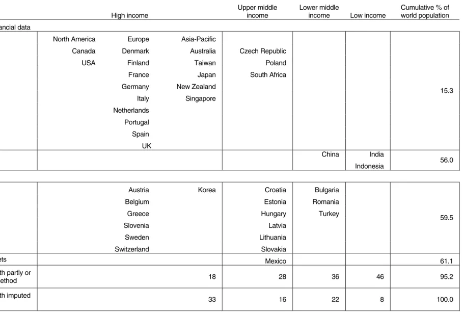
As indicated in Table 1, ‘complete’ financial and non-financial balance sheet data are available for 19 countries. These are all high-income countries, except for the Czech Republic, Poland, and South Africa, which are classed as upper middle-income by the World Bank.6 The data are regarded as ‘complete’ if there is full, or almost full, coverage of financial assets, and inclusion of owner-occupied housing at least on the non-financial side. Sixteen other countries have comparable financial balance sheets, but no information on real assets. This group is less biased towards the rich world since it contains six upper middle income countries and three lower middle income countries. Regional coverage in HBS data is not representative of the world as a whole. Such data tend to be produced at a relatively late stage of development. Europe and North America, and the OECD in general, are well covered, but low-income and transition countries are not.7 In geographic terms this means that coverage is sparse in Africa, Asia, Latin America, and the Caribbean. Fortunately for this study, these gaps in HBS data are offset to an important extent by the availability of survey evidence for the largest developing countries, China, India and Indonesia. Also note that while there are no HBS data for Russia, complete HBS data are available for two European transition countries and financial data for eight others.
As discussed in Appendix I, sources and methods differ across countries, particularly in respect of non-financial assets.8 HBS numbers may be obtained by direct or indirect means. The direct approach involves, for example, estimating the value of owner-
5 The sources and methods for balance sheet and survey data are described in Appendices I and II.
6 The World Bank classification is used throughout the paper except that Brazil, Russia, and South Africa were moved from the lower middle-income category to higher middle-income, and Equatorial Guinea from low to lower middle-income. These changes were prompted by the fact that the WB classifications seems anomalous compared to the Penn World Table GDP data that was used for the year 2000.
7 Interestingly, Goldsmith (1985) prepared ‘planetary’ balance sheets for 1950 and 1978 and found similar difficulties in obtaining representative coverage. He was able to include 15 developed market economies, two developing countries (India and Mexico), and the Soviet Union. This produces a total of 18 countries, one less than the number of countries for which we have complete HBS data for the year 2000.
8 Appendix IIB summarizes key definitional and coverage characteristics of the household balance sheet data by country.
Table 1 Coverage of wealth levels data, year 2000
High income
Upper middle income
Lower middle
income Low income
Cumulative % of world population
Complete financial and non-financial data
Household Balance Sheets North America Europe Asia-Pacific
Canada Denmark Australia Czech Republic
USA Finland Taiwan Poland
France Japan South Africa
Germany New Zealand
Italy Singapore Netherlands Portugal Spain UK 15.3 China India Survey data Indonesia 56.0 Incomplete data
Financial Balance Sheets Austria Korea Croatia Bulgaria
Belgium Estonia Romania
Greece Hungary Turkey
Slovenia Latvia
Sweden Lithuania
Switzerland Slovakia
59.5
Survey data: non-financial assets Mexico 61.1
Number of countries with wealth partly or
fully estimated by regression method 18 28 36 46 95.2
Number of countries with wealth imputed
by mean value of group 33 16 22 8 100.0
occupied housing, or business equity, from survey data. The indirect method may require residual estimation of household assets in which the holdings of other sectors are deducted from national totals obtained from institutional sources. HBS estimates therefore inherit both the errors in data from direct sources, as well as the (possibly large) errors caused by the method of residual estimation.
Often, household balance sheets are compiled in conjunction with the National Accounts or Flow of Funds data, but there are several exceptions. For countries such as New Zealand, Portugal and Spain, data are reported by central banks and include estimates based on Financial Accounts augmented with data on housing assets. The German and Italian data are to a large extent also based on central bank data, but are more complete. The German figures are based on financial accounts data from Deutsche Bundesbank, and non-financial asset information including housing, other real assets and durables. Italian data are based on the financial accounts of the Bank of Italy supplemented by estimates of the stock of dwellings by the Italian statistical office (ISTAT) and of durable goods based on Brandolini et al. (2004). Even if household balance sheets use data from national statistical organizations, they do not necessarily have a broad coverage of non-financial assets. For example, data for the Netherlands are a mix of figures from Statistics Netherlands and the central bank, and the financial balance sheets are only augmented with data on owner-occupied housing. Non-financial data from the Singapore Department of Statistics also cover only housing assets. For Denmark we combined financial balance sheet data with fixed capital stock accounts reported by Statistics Denmark, and for Finland we combined financial balance sheets with estimates of housing assets provided to us by Statistics Finland.
In summary, each of the 19 countries classed as having complete balance sheets report good financial data plus data on owner-occupied housing. Finland, Poland, Singapore, and the Netherlands are at this minimum level. Fifteen countries also report data on some other real property, including land and/or investment real estate in most cases, and six of these countries have estimates for consumer durables.
We considered whether the non-financial coverage in these ‘complete’ balance sheets could be made more uniform by imputing missing items. It is very difficult to devise a satisfactory estimation procedure for land or investment real estate,9 so these items have not been imputed. Since only four countries lack these items entirely, and eight countries, including the USA, have complete data, the impact would not be substantial, although the omissions will have some effect on our results, In contrast, it is reasonably easy to construct estimates of consumer durables, and since this improves the non-financial asset coverage for thirteen countries, these imputations were included.10
9 While balance sheet figures for dwellings also capture the value of land on which they stand, other land is missing for Denmark, Germany, Italy, the Netherlands, and Singapore. Investment or commercial real estate is missing for the Netherlands, New Zealand, Portugal and Singapore, and for Italy (which covers all housing, whether owner occupied or not, but not other real estate). To the best of our knowledge, all real estate and land owned by households is included in the data in all other cases.
10 Durables figures are available for Canada, the USA, Germany, Italy and South Africa. The mean ratio of durables to GDP in Canada and the USA was used to impute durables to Australia, New Zealand, and the UK. For European countries other than the UK, the mean ratio for Germany and Italy was used. Finally, the mean ratio for Canada, the USA, Germany, and Italy was used for imputations for Japan and Singapore.
Appendix IIB also reveals differences in sectoral definition across countries. We aimed for a household sector which covered the assets and debts of households and unincorporated business. However, non-profit organizations (NPOs) are sometimes grouped with households. Data for the UK and USA allowed us to exclude NPOs. This correction is especially important for the USA where NPOs account for about 6 per cent of the financial assets of the household sector (Board of Governors of the Federal Reserve System 2003).
Table 2 reports the asset composition of household balance sheets. The asset composition reflects different influences on household behaviour such as market structure, regulation and cultural preferences (IMF 2005). However, these data need to be analyzed with care, since the comparison may be affected by differences in sectoral definition, asset coverage and estimation methods. For most countries, non-financial assets account for between 40 and 60 per cent of total assets, with higher shares in the Czech Republic, New Zealand, Poland, and Spain. Housing assets constitute a considerable share of non-financial assets. In a number of countries, for example Italy, Spain and the UK, the large increase in real estate prices in the late 1990s helps to explain the high share of housing. The high share of financial assets makes South Africa stand out. One would expect real assets to be important in a developing country, but the well developed financial markets in South Africa, combined with negative rates of return on investment in fixed property and high mortgage interest rates, have resulted in an unusually low share of non-financial assets (see Aron et al. 2006). The USA is also an outlier in the share of financial assets, which is clearly related to the strength of its markets, but may also be partly due to relatively cheap housing and extensive reliance on private pension plans.
The composition of financial assets can be examined not only for the 19 countries with complete balance sheets but also the 16 countries with only financial balance sheets. Striking differences across countries are evident when financial assets are disaggregated into liquid assets, shares and equities, and other assets. Liquid assets are a large part of the total in Japan and in most of the European transition countries. The preference for liquidity in Japan has a long history, but also reflects lack of confidence in real estate and shares after their poor performance in the 1990s (Babeau and Sbano 2003). The share of other financial assets is particularly high in some countries, such as Australia, Austria, the Netherlands, South Africa, and the UK, which may be partly due to the importance of pension fund claims in these countries. Italy stands out as having a particularly low share of liabilities, something that is confirmed by survey data (see below). Poland and the Czech Republic also have low debt ratios, reflecting the under-development of mortgage and consumer credit in European transition countries.
Table 2: Percentage composition of household wealth in household balance sheets, year 2000
Share of total gross assets Share of financial assets financial
assets
non-financial
assets housing liabilities liquid assets equities
other financial assetsa
Household balance sheets
Australia 41 59 20 17 22 20 58 Canada 57 43 20 18 25 32 43 Taiwan 59 41 20 10 39 32 29 Czech Republic 34 66 na 9 60 24 16 Denmark 55 45 24 30 21 31 48 Finland 41 59 48 13 33 45 22 France 40 60 29 11 33 32 35 Germany 40 60 42 16 34 37 29 Italy 42 58 50 3 23 55 21 Japan 50 50 Na 14 53 16 31 Netherlands 54 46 38 16 19 24 57 New Zealand 32 68 59 20 35 40 25 Poland 20 80 62 3 59 25 17 Portugal 49 51 39 19 47 38 15 Singapore 45 55 47 18 44 21 35 South Africa 65 35 16 15 21 19 60 Spain 31 69 60 10 40 43 17 UK 53 47 35 13 20 24 55 USA 67 33 26 15 13 51 36
Financial balance sheets Austria 55 26 19 Belgium 25 59 16 Bulgariab 88 5 7 Croatiab 85 6 9 Estonia 26 54 20 Greece 44 51 4 Hungary 43 43 14 South Korea 61 18 21 Latvia 53 44 3 Lithuania 33 40 27 Romaniab 76 21 3 Slovakiab 74 12 14 Slovenia 52 31 17 Sweden 14 45 40 Switzerland 21 38 41 Turkeyb 62 32 6 Note: a
Other financial assets include insurance and pension reserves and other accounts receivable. b
Composition from year 2004. Source: see Appendix II.
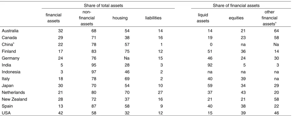
Table 3: Percentage composition of household wealth in survey data, year 2000
Share of total assets Share of financial assets
financial assets
non-financial
assets
housing liabilities liquid
assets equities other financial assetsa Australia 32 68 54 14 14 21 64 Canada 29 71 38 16 19 23 58 Chinab 22 78 57 1 0 na Na Finland 17 83 75 12 51 36 14 Germany 24 76 Na 15 46 24 30 India 5 95 28 3 92 5 3 Indonesia 3 97 46 2 na na na Italy 18 78 69 2 40 39 na Japan 30 70 54 10 59 34 29 Netherlands 21 80 70 27 37 43 20 New Zealand 28 72 37 16 21 21 58 Spain 13 87 58 9 40 38 22 USA 42 58 32 12 15 39 46 Note: a
Other financial assets include insurance and pension plans and other accounts receivable. b
Housing assets are net of associated debts; liabilities exclude housing debt. Source: see Appendix II.
2.2 Survey data
In order to check our HBS data and to expand our sample, especially to non-OECD countries, household wealth survey data were also consulted.11 Country coverage is broader than in HBS data (see Table 3). Most importantly, wealth surveys are available for the three most populous developing (and emerging market) countries: China, India and Indonesia. These three countries, together with Mexico in the case of non-financial assets, are used in regressions in Section 3 that provide the basis for wealth level imputations for our ‘missing countries’.
Like all household surveys, those of wealth are affected by sampling and non-sampling errors. However, these errors are likely to be particularly serious for asset and debts. The high skewness of wealth distributions makes sampling error more severe. Non-sampling error is also a greater problem since differential response (wealthier households are less likely to respond) and misreporting are generally more important than for other variables of interest, such as income. Both sampling and non-sampling error lead to special difficulties in obtaining an accurate picture of the upper tail, which is of course one of the most interesting parts of the wealth distribution (see Davies and Shorrocks 2000: 605-76, 2005).
In order to offset the effects of sampling error in the upper tail, well-designed wealth surveys over-sample wealthier households. This is the practice in the US Survey of Consumer Finances and the Canadian Survey of Financial Security.12 Unfortunately, none of the three countries whose survey data are used in the regressions for financial assets and liabilities reported in the next section over-samples rich households. Sampling error may therefore be of some concern in the Chinese CASS survey, the Indian AIDIS survey (part of the Indian National Sample Survey round 59) and the Indonesian Family Life Survey, despite the high reported response rate (in excess of 90 per cent) in both China and India.
In the case of the Chinese survey, there are additional difficulties regarding the representativeness of the wealth survey sub-sample, which covers only a part of the provinces included in the sample of the State Statistical Bureau (SSB) Household Income Survey. The SSB sample itself also suffers from some degree of geographical under-coverage (Bramall 2001). The Indonesia Family Life Survey has a similar limitation; it samples only 13 of the nation’s 27 provinces, although these include 83 per cent of the country’s population.
11 We use HBS data in preference to survey data wherever the former is available. While HBS data are of course also subject to error, a country’s wealth survey results can be, and normally are, used as an input in creating HBS estimates. Since the HBS estimates benefit from additional inputs of information and data from other sources, they should, in principle, dominate wealth survey estimates. The US Survey of Consumer Finance (SCF) is of such high quality, however, that it is not clear whether US HBS or survey data should be preferred (see, for example, Bertaut and Starr-McCluer 2002: 181-218). Fortunately for our purposes, HBS and SCF estimates of total household wealth in the USA in 2000 are very similar (see below). Our results would differ little if the SCF had been used to establish the USA wealth level.
12 The SCF design explicitly excludes people in the Forbes 400 list of the wealthiest Americans, which again helps to reduce the effects of sampling error; see Kennickell (2006: 19-88).
Aside from the USA—whose sophisticated Survey of Consumer Finance succeeds in capturing most household wealth—surveys usually yield lower totals for most financial assets compared with HBS data, principally due to the lower response rate of wealthy households and under-reporting by those who do respond.13 In contrast, non-financial assets, especially housing, are sometimes better covered in survey data. The relative importance of different types of assets at different stages of development is reflected in the survey coverage. The Finnish survey, for example, focuses on financial assets, housing and vehicles. The surveys from the three developing countries pay relatively little attention to financial wealth, since it is of less importance, and concentrate instead on housing, agricultural assets, land and consumer durables.
Table 3 reports asset composition in the survey data. It is clear that non-financial assets bulk larger in surveys than in HBS data, reflecting both the relative accuracy of housing values in survey data and the importance of non-response and under-reporting by rich households, who own a disproportionate share of financial assets. The table also highlights the relative importance of financial and non-financial assets in developed and developing countries. The two low-income countries in our sample, India and Indonesia, stand out as having particularly high shares of non-financial wealth.14 This is no surprise since assets such as housing, land, agricultural assets and consumer durables are particularly important in developing countries. In addition, financial markets are often primitive. In India, the only low or middle income country for which the composition of financial assets is reported in Table 3, most of the financial assets owned by households are liquid. Renwei and Sing (2005) report more detailed data for urban areas of China, showing that about 64 per cent of household financial assets are liquid. In Table 3, China does not stand out as having a high share of non-financial assets. One reason is that the value of housing is reported net of mortgage debt in China. Another is that there is no private ownership of urban land. And of course there has been rapid accumulation of financial assets by Chinese households in recent years. The ratio of liabilities to total assets is particularly low in India and Indonesia (for China only non-housing liabilities are reported). Again poorly developed financial markets help to explain this phenomenon. But, in addition, underreporting of debt appears to be more severe than underreporting of assets. Subramanian and Jayaraj (2006) estimate that debts are, on average, underrepresented in the AIDIS by a factor of almost three. Italy also stands out as having a very low share of liabilities. This low share echoes the finding in HBS data, and likely reflects the relative lack of mortgage loans in Italy compared to other high income OECD countries.
13 Statistical organizations fight these forms of non-sampling error through their survey technique and questionnaire design. Once the results are in, it is also possible to try to correct for these errors. Ambitious efforts have been made in the Italian SHEW survey. Brandolini (2004) uses records of the number of contacts needed to win a response to estimate the differential response relationship, which allows reweighting of the sample. He also uses results of a validation study comparing survey responses and institutional records to correct for misreporting of selected financial assets. Finally, this study also imputes non-reported dwellings owned by respondents (aside from their principal dwelling).
14 This echoes the findings of Goldsmith (1985) who reported that India and Mexico had an average of 65 per cent of national assets in tangible form in 1978, compared to 51 per cent for fourteen developed market economies.
Combining the balance sheet and survey data, it is evident that there are major international differences in asset composition. Real property, particularly land and farm assets, are more important in less developed countries, while financial assets are more important in rich countries. There are also major international differences in the types of financial assets owned. Savings accounts are favoured in transition economies and some rich Asian countries, while share-holdings and other types of financial assets are more evident in rich western countries. Debt is also less important in developing and transition countries than in the more developed countries (with the notable exception of Italy).
2.3 Wealth levels from household balance sheet and survey data
When wealth levels are compared across countries, one of the first issues to be confronted is the appropriate rate of exchange between currencies. In comparisons of consumption or income there is widespread agreement that international price differences should be taken into account via the use of PPP exchange rates.15 This procedure seems appropriate for wealth holdings also if the focus of attention is, say, the bottom 95 per cent of wealth-holders, for whom domestic prices are the main determinant of the real value of their assets. However, a large share of wealth is held by households in the top few percentiles of the distribution. People in this category, and their financial assets, tend to be internationally mobile, making exchange rates more relevant for international wealth comparisons among the rich and super-rich.
This paper follows the convention of using PPP exchange rates to compare countries; unless otherwise stated, all wealth figures are expressed in PPP US dollars for the year 2000. Selected comparable figures on an exchange rate basis are presented in footnotes and appendices. They are also discussed in detail in Davies et al. (2007) which places more emphasis on the upper tail of the distribution.
Table 4 summarizes information on the per capita wealth and income of countries with complete household balance sheet or wealth survey data(data for individual countries are given in Appendix III). Of the 19 countries that have complete HBS data, the USA ranks first with per capita wealth of $143,727 in 2000, followed by the UK at $128,959, Japan at $124,858, the Netherlands at $121,165, Italy at $120,897, and then Singapore at $113,631. South Africa is in last place, at $16,266, preceded by Poland at $24,654, and the Czech Republic at $32,431. The overall range is rather large, with per capita wealth in the USA 8.8 times as great as that of South Africa. The (unweighted) coefficient of variation (CV) among the 19 countries is 0.440.
15 There is, however, some disagreement about the type of PPP exchange rates that should be used. We follow common practice and use the Penn World Table PPP rates, which are based on the ’Geary’ method. This method has many practical advantages, including desirable adding-up properties but has been criticized in the past for its lack of a rigorous theoretical basis. The leading competitor is the ‘EKS’ method, which has a stronger theoretical foundation. The EKS method has been used by the OECD and Eurostat to compare income across their member countries. Recently, Neary (2004) has clarified the theoretical basis for the Geary method.
Table 4: Wealth per capita from household balance sheet and survey data, year 2000
US$ per capita at PPP exchange rates US$ per capita at official exchange rates
Wealtha Real GDPb Personal disposable incomec Real Consumptionb Wealtha GDPb Personal disposable incomec Consumptionb
Household balance sheet data
Mean 84955 22519 13482 14240 74890 19434 11530 12239
Median 90906 23917 12798 15197 70916 21425 11915 12708
Coefficient of variation 0.440 0.301 0.331 0.319 0.612 0.527 0.524 0.521
Highest wealth: USA 143727 35619 25480 24313 143727 35619 25480 24313
Lowest wealth: South Africa 16266 8017 4691 5210 5977 2946 1724 1914
Survey data
Mean 59349 20311 12338 13072 53251 17983 10911 11588
Median 61218 23917 12798 15197 45176 20338 11557 12708
Coefficient of variation 0.667 0.512 0.551 0.530 0.836 0.669 0.707 0.671
Highest wealth: USA 143857 35619 25480 24313 143857 35619 25480 24313
Lowest wealth: India 6513 2684 1916 1406 1112 458 327 240
Ratio high/low - HBS 8.8 4.4 5.4 4.7 24.1 12.1 14.8 12.7
Ratio high/low - survey data 22.1 13.3 13.3 17.3 129.4 77.8 77.9 101.4
China/USA - survey data 12.8 9.3 13.2 13.0 55.1 40.0 56.8 56.1
Note: a
See Appendix II for sources of HBS and survey data. Figures have been adjusted to year 2000 values using the real growth rate per capita. b
Source: Penn World Table 6.1. c
The next column shows GDP per capita. In the group of 19 countries with HBS data, the USA again ranks first, at $35,619, and South Africa last, at $8,017. However, the range is much smaller than for net worth per capita. The ratio of highest to lowest GDP per capita is only 4.4, and the coefficient of variation (again among the 19 countries) is 0.301, compared to 0.440 for net worth per capita. These results are a first illustration of the fact that, globally, wealth is more unequally distributed than income. The comparison here is only between countries. The full results we present later in the paper include inequality within countries, which further increases the gap between income and wealth inequality.
Column four shows personal disposable income per capita for the same group of countries. The USA again ranks first, at $25,480, South Africa is again last, at $4,691, and the ratio of highest to lowest is 5.4, slightly higher than for GDP per capita. The coefficient of variation is 0.333, again slightly higher than that of GDP per capita. The fifth column shows real consumption per capita, whose dispersion is intermediate between that of GDP and disposable income. All in all, the per capita variation of net worth is much greater than that of GDP, disposable income or consumption.
Differences across countries are even more pronounced in survey data due to the inclusion of China, India, and Indonesia. Of the 13 countries with the pertinent data, the USA again ranks first in net worth per capita, at $143,857, followed by Australia at $101,597, and Japan at $91,856. In this group, India and Indonesia occupy the bottom two positions, at $6,513 and $7,973, respectively. China appears to be about twice as wealthy as India, having per capita net worth of $11,267. Note that the PPP adjustment has a proportionately greater impact on the figures for developing countries. Using official exchange rates, all three countries have much lower per capita wealth: India at $1,112, Indonesia at $1,440, and China at $2,613. Hence inequality in wealth between countries is greater using official exchange rates, as reflected in the CV of 0.612 shown in the table versus 0.440 on a PPP basis. In the survey data, as in the HBS data, the range in per capita wealth is much larger than that of per capita GDP, disposable income, or consumption. The ratio of highest to lowest is 22 for wealth per capita, 13 for both GDP and disposable income, and 17 for consumption. The coefficients of variation for the income and consumption variables are again smaller than for wealth, and higher using official exchange rates than PPP rates.
As would be expected, wealth is fairly highly correlated with both income and consumption. The correlation between net worth and GDP is 0.77 in the HBS data and is higher again in the survey data at 0.87. Correlations of wealth and disposable income are higher from both HBS and survey sources—rising to 0.94 in the survey data—while correlations of wealth with consumption are a little lower: 0.71 from balance sheet data and 0.89 from survey data. The highest correlations are found between the logarithms of net worth per capita and disposable income per capita: 0.91 from the balance sheet data and 0.97 from the survey data. The correlations of log wealth per capita and log consumption per capita are slightly lower.16
16 See Appendix IV. When official exchange rates are employed, the correlations are uniformly higher, but the pattern is similar.
3 Imputing wealth levels to other countries
The next step is to generate per capita wealth values for the remaining countries of the world. As explained below, regressions run on the 38 countries with HBS or survey data enable part or all of wealth to be estimated for many countries. This yields a total of 150 countries with observed or estimated wealth, covering 95.2 per cent of the world’s population in 2000. It is tempting to regard the results as representative of the global picture. However this would implicitly assume that the 79 excluded countries are neither disproportionately rich nor poor, an untenable assumption. While the omitted countries include several small rich nations (for example, Liechtenstein, the Channel Islands, Kuwait, Bermuda), the most populous countries in the group (Afghanistan, Angola, Cuba, Iraq, North Korea, Myanmar, Nepal, Serbia, Sudan, and Uzbekistan, each have more than 10 million population) are all classified as low income or lower middle income. To try to compensate for this bias towards poorer nations, each of the excluded countries was assigned the mean per capita wealth of the appropriate continental region (6 categories) and income class (4 categories)17. This imputation is admittedly crude, but nevertheless an improvement over the default of simply disregarding the excluded countries. It allows us, in the end, to assign wealth levels to 229 countries.
The regressions reported below are designed to predict wealth in countries where wealth data are missing. The goal is not to estimate a structural model of wealth-holding, but to find equations that fit well in-sample and that will also allow us to predict out-of-sample. The nature of this exercise limits the range of models that can be applied. Perhaps most importantly, it limits the choice of explanatory variables to those that are available not only for the countries with wealth data but also for a large number of countries without wealth data.
3.1 Wealth regressions
The first experiment considered OLS regressions for those countries with complete wealth data, excluding the 17 countries with incomplete data shown in Table 1. Initially the dependent variable was per capita wealth and the principal independent variable was per capita income or consumption. As Figures 1 and 2 indicate, there is a strong relationship between wealth and income, so these equations fit fairly well.18 However, there are significant gains from the greater flexibility offered by running separate regressions for (i) non-financial assets, (ii) financial assets, and (iii) liabilities. The improvement is due in part to the fact that certain variables help explain one or two of the components, but not all three. In addition, the relative impact of common variables varies across the equations.
17 Our regional calculations treat China and India separately due to the size of their populations. In the regional breakdowns it was also convenient to distinguish the high income subset of countries in the Asia-Pacific region (a list which includes Japan, Taiwan, South Korea, Australia, New Zealand, and several middle eastern states) from the remaining (mainly low-income) nations.
18 Figure 1 uses wealth from the HBS data while Figure 2 uses wealth from survey data. The slope of the simple regression line in Figure 2 is lower than that in Figure 1, reflecting the fact that survey data generally provide lower estimates of wealth than do national balance sheets.
Running separate regressions for the three components enables data to be used from countries lacking complete wealth data. Observations for both financial assets and liabilities are available for the 16 countries shown in Table 1 with financial balance sheets, but no data on real assets. In addition, Mexico provides an observation of non-financial assets. Adding these observations not only increases the sample size, but also brings in more developing and transition countries, thus improving the ability of the regressions to predict the wealth of the ‘missing’ countries.
The dependent variable is calculated from household balance sheet data for 35 countries and survey data for four countries that lack HBS data (China, India, Indonesia, and Mexico). The income variable is very important in each regression. Although the best fit is obtained using disposable income per capita (see the results in Appendix V), real consumption per capita reduces goodness of fit only slightly and is preferred for our purposes since it is available for about twice as many countries.
Because errors in our three equations are likely to be correlated, we explored application of the seemingly unrelated regressions (SUR) technique due to Zellner (1962) (see Greene 1993: 486-99). This involves stacking equations and estimating via generalized least squares. While OLS estimates are consistent, SUR provides greater efficiency, with the gain in efficiency increasing with the correlation of the errors across the equations, and decreasing with the correlation of the regressors used in the different equations. For equations with an unequal number of observations it is not straightforward to apply SUR. Since we have an equal number of observations for financial assets and liabilities, but fewer observations for non-financial assets, and since we believe errors are more likely to be correlated between financial assets and liabilities than between the latter variables and non-financial assets, we have applied SUR here only for financial assets and liabilities.19
19 While it is theoretically possible to apply SUR with an unequal number of observations in the equations estimated, this is very difficult to do in STATA or in other standard packages. Errors in the financial assets and liabilities equations are likely to be correlated, but error-correlation between either of those variables and non-financial assets is likely to be smaller, since estimates of the latter generally come from different sources and are prepared using different techniques. Thus correlations in measurement error, at least, should be small.
Figure 1: Wealth from household balance sheet versus disposable income, PPP$
Figure 2: Wealth from surveys versus disposable income, PPP$
AUS CAN CHN FIN GER IND IDN ITA JPN NLD NZLESP USA 50000 100000 150000 200000
Wealth per capita (PPP$)
0 5000 10000 15000 20000 25000
Personal disposable income per capita (PPP$) AUSCAN CZE DNK FIN FRAGER ITAJPN NLD NZL POL PRT SGP ZAF ESP UK USA 50000 100000 150000 2 000 00
Wealth per capita (PPP$)
0 5000 10000 15000 20000 25000
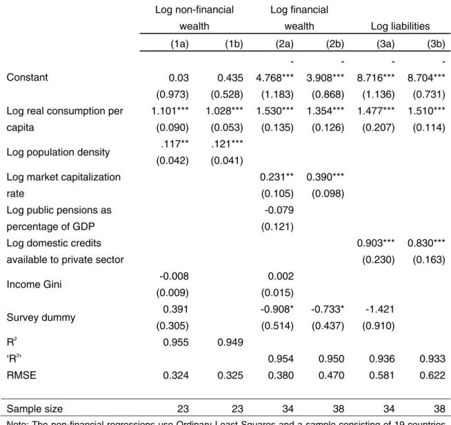
Table 5: Regressions of wealth components
Independent variables Dependent variables
Log non-financial wealth
Log financial
wealth Log liabilities
(1a) (1b) (2a) (2b) (3a) (3b)
0.03 0.435 -4.768*** -3.908*** -8.716*** -8.704*** Constant (0.973) (0.528) (1.183) (0.868) (1.136) (0.731) 1.101*** 1.028*** 1.530*** 1.354*** 1.477*** 1.510***
Log real consumption per
capita (0.090) (0.053) (0.135) (0.126) (0.207) (0.114)
.117** .121***
Log population density
(0.042) (0.041)
0.231** 0.390***
Log market capitalization
rate (0.105) (0.098)
-0.079 Log public pensions as
percentage of GDP (0.121)
0.903*** 0.830*** Log domestic credits
available to private sector (0.230) (0.163)
-0.008 0.002 Income Gini (0.009) (0.015) 0.391 -0.908* -0.733* -1.421 Survey dummy (0.305) (0.514) (0.437) (0.910) R2 0.955 0.949 ‘R2 ’ 0.954 0.950 0.936 0.933 RMSE 0.324 0.325 0.380 0.470 0.581 0.622 Sample size 23 23 34 38 34 38
Note: The non-financial regressions use Ordinary Least Squares and a sample consisting of 19 countries with HBS data and 4 with survey data. The financial assets and liabilities regressions use the Seemingly Unrelated Regression (SUR) method and a sample consisting of 35 countries with HBS or financial balance sheet data and 3 with survey data. Lack of data on public pensions reduces the sample size by 4 in specifications (2a) and (3a). Standard errors are given in parentheses. Significance: * 10% level; ** 5% level; *** 1% level.
Sources: (a) Market capitalization rate, public spending on pensions as a percentage of GDP, and availability of domestic credit are from World Development Indicators 2005. (b) Real consumption and GDP per capita are from PWT 6.1. See Alan Heston, Robert Summers and Bettina Aten, Penn World Table Version 6.1, Center for International Comparisons at the University of Pennsylvania (CICUP), October 2002. For countries not available in PWT 6.1, GDP per capita is taken from the United Nations Common Database (2006). (c) Income Gini is from WIIDA2a. See UNU-WIDER World Income Inequality Database, Version 2.0a, June 2005. (d) Personal disposable income is from the EIU. See The Economist Intelligence Unit (2005), WorldData.(e) Population is taken from the United Nations Common Database (2006).
Table 5 shows the results with two different versions of the consumption specification, labelled a and b. The preferred specification is b in all three cases. Both the dependent variables and most of the independent variables are entered in log form. Note first that the logarithm of real consumption per capita appears significant at the 1 per cent level in all of the runs. The estimated elasticities of non-financial and financial wealth with respect to consumption are 1.028 and 1.354 respectively in the preferred runs. The slightly greater elasticity for financial wealth seems plausible, since higher income countries tend to have better developed financial markets. There is an even larger difference for liabilities, which have an estimated elasticity of 1.510. These differences in consumption elasticities imply that, for the many low income countries with assigned wealth values, imputed financial assets and (especially) liabilities will tend to be relatively less important than non-financial assets.
A dummy variable for the data source (HBS or survey data) was tried in all three regressions, but found to be insignificant in the equation for non-financial assets, not unexpectedly since survey data typically cover non-financial assets quite well. While insignificant in the first liabilities specification, and therefore dropped from run b for liabilities, the survey dummy is significant at the 10 per cent level in both runs for financial wealth. With a value of -0.733 in the b run, this dummy reflects the well-known fact that financial assets are under-reported and under-represented in survey data. Five other independent variables were also considered:20
Population density: The value of non-financial assets, particularly housing, should be positively related to the degree of population density (greater density indicating a relative scarcity of land). This variable is statistically significant in the non-financial asset equation.
Market capitalization rate: The value of household financial assets should be positively correlated with this measure of the size of the stock market. It is positive and significant in both regressions for financial wealth. This is a useful result in terms of prediction and imputations, since the variable is available for a large number of countries that do not have full wealth data.
Public spending on pensions as a percentage of GDP: This was expected to be negatively related to financial assets per capita, since public pensions may substitute for private saving. However, the variable was not statistically significant and was dropped in the b specification.
Income Gini: Some theoretical models suggest that income inequality and per capita wealth are positively related. However, the variable turned out to be insignificant.
Domestic credits available to the private sector: This variable is highly significant in the liabilities regression, which is fortunate from the imputation perspective since, as in the
20 The log form was used for most of the variables. The lowest positive value in the sample was imputed when the values were negative or zero.
case of market capitalization, the variable is available for many of our ‘missing countries’. The R2 or ‘R2’ for each equation indicates that the model fits fairly well.21 3.2 Estimated wealth levels
Table 6 summarizes the wealth levels obtained for the world and its regions. HBS data are used where available (see Table 1); survey data are used for China, India and Indonesia. Financial assets and liabilities are imputed for 112 countries, and financial assets for 127 countries, using the regressions described in the previous section. As explained earlier, the 79 ‘excluded’ countries that do not have the required data for the regression-based estimation were assigned the mean per capita wealth level of their respective region and income class.
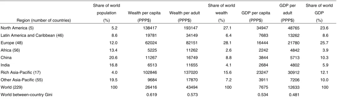
Table 6 provides both per capita and per adult numbers.22 For the world as whole in 2000, net worth was $26,416 per capita and $43,494 per adult. North America accounted for 27 per cent of world household wealth, much more than its 5 per cent share of world population and greater than its 24 per cent share of world GDP. The ‘rich Asia-Pacific’ group and Europe show a similar pattern, with wealth shares much greater than their population shares and larger than their shares of world GDP.23 Given these results, it is not surprising to see that between-country inequality, as shown by the Gini coefficient, is higher for wealth than GDP (0.619 vs. 0.534 respectively on a per capita basis). Note also that between-country wealth inequality is lower using the per adult basis (which gives a Gini of 0.573), reflecting the fact that the difference between wealth per capita and per adult is greater in poor countries, which have a higher proportion of children in their populations.
The rich Asia-Pacific group includes Hong Kong, which has the highest mean wealth in the world on either a per capita or a per adult basis according to our estimates— $188,699 per capita and $246,307 per adult, or 5.7 times the world average per adult (see Appendix VI as well as Table 6). This group also includes Japan and Singapore, both at 3.6 times the world average per adult. Europe contains both very high wealth countries, such as Luxembourg (the second place country, very slightly behind Hong Kong and also with wealth 5.7 times the world average), the UK (4.0 times the world average), and the Netherlands and Italy (3.7 and 3.4 times the world average respectively), as well as low wealth countries such as Moldova (27 per cent of the world average), the Ukraine (30 per cent), and Albania (41 per cent).
21 R2
is not a well-defined concept in generalized least squares, so as is customary the fraction of the variance in the dependent variable that is ‘explained’ in each regression is referred to as ‘R2’ here.
22 While per capita magnitudes are more familiar, we argue in the next section that it is best to analyze the world wealth distribution among adults rather than all individuals. It is therefore helpful to begin looking at per adult, as well as per capita, figures at this point.
23 Note that the disproportion between wealth and population shares, although large, is less for Europe than the other high wealth regions. This reflects in part the inclusion of the lower wealth countries of Eastern Europe.
Table 6: Average wealth by region, year 2000
Region (number of countries)
Share of world population
(%)
Wealth per capita (PPP$)
Wealth per adult (PPP$) Share of world wealth (%) GDP per capita (PPP$) GDP per adult (PPP$) Share of world GDP (%) North America (5) 5.2 138417 193147 27.1 34947 48765 23.6
Latin America and Caribbean (46) 8.6 19781 34149 6.4 7683 13262 8.6
Europe (48) 12.0 62024 82151 28.1 16444 21780 25.7 Africa (56) 13.4 5225 11262 2.6 2242 4842 3.9 China 20.6 11267 16749 8.8 3844 5713 10.3 India 16.8 6513 11655 4.1 2684 4802 5.9 Rich Asia-Pacific (17) 4.0 102846 137020 15.6 23247 30912 12.1 Other Asia-Pacific (55) 19.5 9684 17870 7.2 3911 7206 10.0 World (229) 100 26416 43494 100 7675 12633 100
World between-country Gini 0.619 0.573 0.534 0.481
Note: The world between-country Gini refers to the Gini inequality value computed using the per capita (or adult) wealth (or income) figures for 229 countries weighted by population size.
Lower down the scale, China and India collectively accounted for 37 per cent of world population in the year 2000, but only 16 per cent of world GDP and 13 per cent of the global wealth. China’s net worth per adult was $16,749 (39 per cent of the world average) and India’s was $11,655 (27 per cent). Latin American and the Caribbean had 9 per cent of the world’s population and GDP, but 7 per cent of world wealth. Among this group, the wealthiest countries were Barbados (3.3 times the world average per adult), Puerto Rico (2.6 times), and Trinidad and Tobago (1.9 times). The less affluent countries in this group include Peru (48 per cent of the world average), Colombia (56 per cent) and Venezuela (60 per cent).
Africa and ‘other Asia-Pacific’ countries together accounted for 33 per cent of the world population but only 14 per cent of world GDP and 10 per cent of global wealth. All countries in the other Asia-Pacific group have net worth per adult below the world average, ranging from Turkey (88 per cent of the world average) and Saudi Arabia (99 per cent) at the high end of the scale to Yemen (8 per cent), Cambodia (25 per cent), Vietnam (23 per cent), and Pakistan (29 per cent) at the other end. With the notable exception of Mauritius and the Seychelles (2.1 and 1.1 times the world average per adult), the African nations are all below average in per capita wealth and include South Africa (67 per cent of the world average), Zimbabwe (32 per cent), Kenya (18 per cent), Uganda (17 per cent), Tanzania (6 per cent), and Nigeria (5 per cent).
4 Wealth distribution within countries
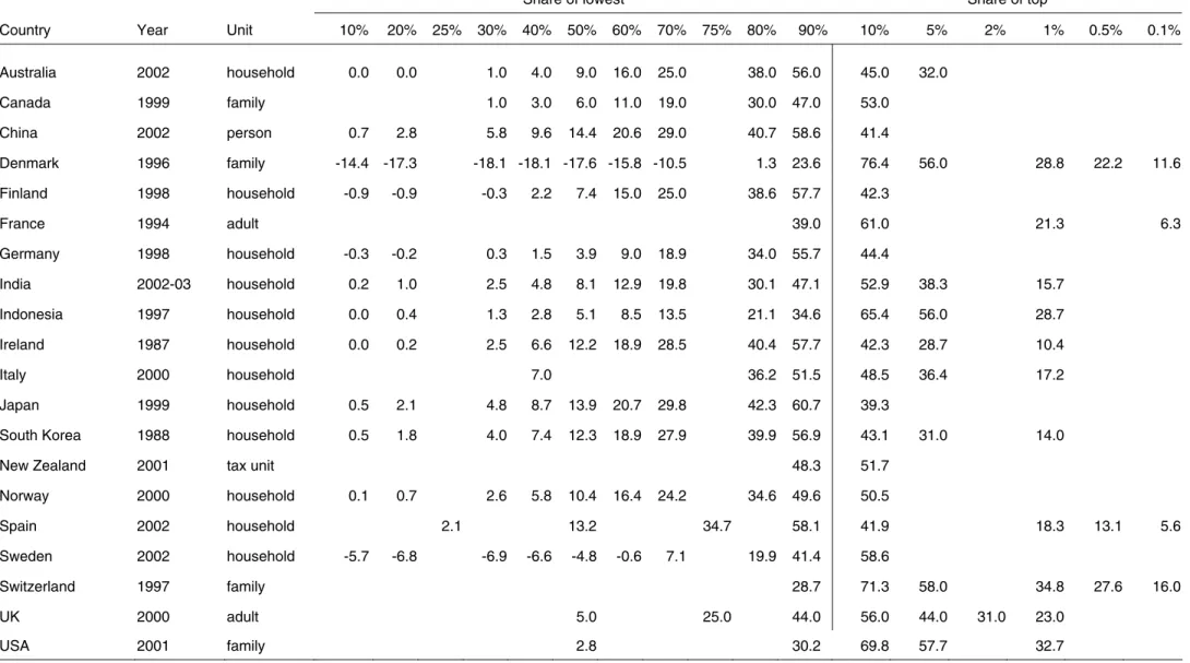
As indicated in Table 7, information on the distribution of wealth across households or individuals can be assembled for 20 countries. One set of figures was selected for each nation, with a preference for the year 2000, ceteris paribus. To assist comparability across countries, a common distribution template was adopted, consisting of the decile shares reported in the form of cumulated quantile shares (i.e. Lorenz curve ordinates) plus the shares of the top 10 per cent, 5 per cent, 2 per cent, 1 per cent, 0.5 per cent and 0.1 per cent.
The data differ in many significant respects. The economic unit of analysis is most often a household or family, but sometimes individuals or, in the case of the UK, adult persons. Distribution information is usually reported for the share of wealth owned by each decile, together with the share of the top 5 per cent and the top 1 per cent of wealth-holders. But this pattern is far from universal. In some instances information on quantile shares is very sparse. On other occasions, wealth shares are reported for the top 0.5 per cent or even the top 0.1 per cent in the cases of Denmark, France, Spain, and Switzerland.
Table 7: Wealth shares for countries with wealth distribution data
Share of lowest Share of top
Country Year Unit 10% 20% 25% 30% 40% 50% 60% 70% 75% 80% 90% 10% 5% 2% 1% 0.5% 0.1%
Australia 2002 household 0.0 0.0 1.0 4.0 9.0 16.0 25.0 38.0 56.0 45.0 32.0 Canada 1999 family 1.0 3.0 6.0 11.0 19.0 30.0 47.0 53.0 China 2002 person 0.7 2.8 5.8 9.6 14.4 20.6 29.0 40.7 58.6 41.4 Denmark 1996 family -14.4 -17.3 -18.1 -18.1 -17.6 -15.8 -10.5 1.3 23.6 76.4 56.0 28.8 22.2 11.6 Finland 1998 household -0.9 -0.9 -0.3 2.2 7.4 15.0 25.0 38.6 57.7 42.3 France 1994 adult 39.0 61.0 21.3 6.3 Germany 1998 household -0.3 -0.2 0.3 1.5 3.9 9.0 18.9 34.0 55.7 44.4 India 2002-03 household 0.2 1.0 2.5 4.8 8.1 12.9 19.8 30.1 47.1 52.9 38.3 15.7 Indonesia 1997 household 0.0 0.4 1.3 2.8 5.1 8.5 13.5 21.1 34.6 65.4 56.0 28.7 Ireland 1987 household 0.0 0.2 2.5 6.6 12.2 18.9 28.5 40.4 57.7 42.3 28.7 10.4 Italy 2000 household 7.0 36.2 51.5 48.5 36.4 17.2 Japan 1999 household 0.5 2.1 4.8 8.7 13.9 20.7 29.8 42.3 60.7 39.3
South Korea 1988 household 0.5 1.8 4.0 7.4 12.3 18.9 27.9 39.9 56.9 43.1 31.0 14.0
New Zealand 2001 tax unit 48.3 51.7
Norway 2000 household 0.1 0.7 2.6 5.8 10.4 16.4 24.2 34.6 49.6 50.5 Spain 2002 household 2.1 13.2 34.7 58.1 41.9 18.3 13.1 5.6 Sweden 2002 household -5.7 -6.8 -6.9 -6.6 -4.8 -0.6 7.1 19.9 41.4 58.6 Switzerland 1997 family 28.7 71.3 58.0 34.8 27.6 16.0 UK 2000 adult 5.0 25.0 44.0 56.0 44.0 31.0 23.0 USA 2001 family 2.8 30.2 69.8 57.7 32.7
The most important respect in which the data vary across countries is the manner by which the information is collected. Household sample surveys are employed in 15 of the 20 countries.24 Survey results are affected by sampling and non-sampling error, as discussed earlier. Non-sampling error tends to reduce estimates of inequality and the shares of the top groups because wealthy households are less likely to respond, and because under-reporting is particularly severe for the kinds of financial assets that are especially important for the wealthy—for example, equities and bonds.
Other wealth distribution estimates derive from tax records. The French and UK data are based on estate tax returns, while the data for Denmark, Norway, and Switzerland originate from wealth tax records. These data sources have the advantage that ‘response’ is involuntary, and under-reporting is illegal. However, under-reporting may occur nonetheless, and there are valuation problems that produce analogous results. Wealth tax regulations may assign to some assets a fraction of their market value, and omit other assets altogether. There are also evident differences in the way that debts are investigated and recorded. For most countries the bottom decile of wealth-holders is reported as having positive net wealth, but in Sweden the bottom three deciles each have negative net worth and in Denmark this is true for the bottom four deciles.25
Table 7 shows that estimated wealth concentration varies significantly across countries and is generally very high. Comparisons of wealth inequality often focus attention on the share of the top 1 per cent. That statistic is reported for 11 countries, a list that excludes China, Germany, and the Nordic countries apart from Denmark. Estimated shares of the top 1 per cent range from 10.4 per cent in Ireland to 34.8 per cent in Switzerland, with the USA towards the top end of this range at 32.7 per cent.26 The share of the top 10 per cent, which is available for all 20 countries, ranges from 39.3 per cent in Japan to 76.4 per cent in Denmark.
The differences in wealth concentration across countries in Table 7 are probably attributable in part to differences in data quality. If survey data do not oversample the upper tail, the shares of the richest groups can be depressed very significantly (see, for example, Davies 1993): in the absence of corrections for non-sampling error, a reasonable guess is that the share of the top 1 per cent may be under-estimated by about
24 The list of countries differs a little from that used in Sections 2 and 3. Here the desire is to exploit distributional information for as many countries as possible, so countries with data considerably earlier than 2000 were added: Ireland (for 1987) and Korea (for 1988). It is hoped that the shape of wealth distribution in these countries was reasonably stable from the late 1980s to the year 2000, even if it is unsafe to use the 1980s values for wealth levels. Sweden was also added since its distributional detail is of interest, although the mean from this source was not judged sufficiently reliable to be used in our estimates of wealth levels. The Netherlands was dropped due to insufficient distributional detail.
25 Klevmarken (2006: 276-94) identifies a number of factors that helped to account for negative wealth shares of Swedish households in the tax register data in the 1990s, and may still have been operative in 2002. These include student loan debt, the inclusion of debt incurred to buy assets that are not covered in the data (mainly consumer durables) and a household definition in which young adults living at home with their parents, as well as unmarried cohabiting adults, were counted as separate households.
26 The sampling frame for the USA survey excludes the Forbes 400 richest families; adding them would raise the share of the top 1 per cent by about two percentage points; see Kennickell (2006: 20).
5–10 percentage points. The surprisingly low top shares seen here in Australia, Ireland, and Japan may well reflect this phenomenon. One way to attack this problem is to replace, where possible, the survey estimate of the upper tail with figures derived from lists of the very rich (and their wealth) compiled by journalists and others (see Atkinson (2006) for discussion of this form of evidence). While estimates have been prepared on this basis in a few countries, the approach has not been widely adopted and is beyond the scope of this paper.
As evident from Table 7, the available sources provide a patchwork of quantile shares. In order to move towards an estimate of the world distribution of wealth, more complete and comparable information is needed on the distribution in each country. To achieve this, missing cell values were imputed using a programme developed at UNU-WIDER which constructs a synthetic sample of 1000 observations that conforms exactly with any valid set of quantile shares derived from a distribution of positive values (e.g., incomes) (see Shorrocks and Wan 2007.) To apply this ‘ungrouping’ programme, the negative wealth shares reported for Denmark, Finland, Germany, and Sweden were discarded, together with the zero shares reported elsewhere, thus treating the cell values as missing observations.
The 20 countries for which wealth distribution data are available include China and India, and hence cover a good proportion of the world population. They also include most of the large rich countries, and hence cover much of global wealth. However, the fact that the list is dominated by OECD members cautions against extrapolating immediately to the rest of the world.
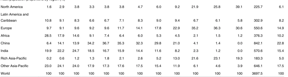
For most countries lacking direct wealth distribution data, the pattern of wealth distribution was estimated using income distribution data recorded in the WIID dataset, on the grounds that wealth inequality is likely to be correlated—possibly highly correlated—with income inequality across countries. The WIID dataset covers 144 countries and has multiple observations for most of them. Where possible, data was chosen for household income per capita across individualsfor a year close to 2000, with first priority given to figures on disposable income, then consumption or expenditure. Eighty-five per cent of the income distributions conform to these criteria. Figures for gross incomes added a further seven per cent, leaving a residual eight per cent of countries for which the choices were very limited. The ‘ungrouping’ programme was then used to generate quantile shares for income (reported in Lorenz curve form) according to the same template employed for wealth distribution.
The common template applied to the wealth and income distributions allows Lorenz curve comparisons for each of the 20 reference countries listed in Table 7. In every instance, wealth shares are lower than income shares at each point of the Lorenz curve: in other words, wealth is unambiguously more unequally distributed than income. Furthermore, the ratios of wealth shares to income shares at various percentile points appear to be fairly stable across countries, supporting the view that income inequality is a good proxy for wealth inequality when wealth distribution data are not available. Thus, as a first approximation, it seems reasonable to assume that the ratio of the Lorenz ordinates for wealth compared to income are constant across countries, and that these constant ratios (14 in total) correspond to the average value recorded for the 20
reference countries.27 This generates estimates of wealth distribution for 124 countries to add to the 20 original countries which have direct evidence of wealth inequality. The group of 144 countries with actual or estimated wealth distribution data differs slightly from the group of 150 nations which have figures for mean wealth derived from actual data or the regressions of Section 3. Distributional evidence is more common for populous countries, so the group of 144 now includes Cuba, Iraq, Myanmar, Nepal, Serbia, Sudan, and Uzbekistan, and covers 96.6 per cent of the global population. For the rest of the world not covered by WIID data, the default of disregarding the remaining countries was again eschewed in favour of imputing a wealth distribution pattern equal to the (population weighted) average for the corresponding region and income class.
5 World distribution
The final step in the construction of the global distribution of wealth combines the national wealth levels derived in Section 3 with the wealth distribution data derived in Section 4. Specifically, the ungrouping programme was applied to each country to generate a sample of 1,000 synthetic individual observations consistent with the (actual, estimated or imputed) wealth distribution. These were scaled up by mean wealth, weighted by the adult population size of the respective country, and merged into a single dataset comprising over 200,000 observations.28 The complete sample was then processed to obtain the minimum wealth and the wealth share of each percentile in the global distribution of wealth. The procedure also provides estimates of the composition by country of each wealth percentile, although these are rough estimates given that the population of each country is condensed into a sample of 1,000, so that a single sample observation for China or India represents more than half a million adults.
The interpretation of data on personal wealth distribution hinges a great deal on the underlying population deemed to be relevant. Are we interested in the distribution of wealth across all individuals, adult persons, or households or families?29 When examining the analogous issue of global income distribution, it is common practice to assume (as a first approximation) that the benefits of household expenditure are shared equally among household members, and that each person should be weighted equally in the overall distribution. However, the situation with wealth is rather different. Personal assets and debts are typically owned by named individuals, and may well be retained by those individuals if they leave the family. Furthermore, while some household assets, especially housing, provide a stream of communal benefits, it is highly unlikely that control of assets is shared equally by household members or that household members will share equally in the proceeds if the asset is sold. Membership of households can be quite fluid (for example, with respect to children living away from home) and the pattern of household structure varies markedly across countries. For these and other
27 To circumvent aggregation problems, the adjustment ratio was applied to the cumulated income shares (i.e. Lorenz values) rather than separate quantile income shares.
28 There are 229 countries in total, but a number of small countries with identical imputed wealth levels and distributions were merged at this point.