Identifying Asset Poverty Thresholds New methods with an application to Pakistan and Ethiopia

Identifying Asset Poverty Thresholds – New methods

with an application to Pakistan and Ethiopia

Felix Naschold Cornell University

Department of Applied Economics and Management 214 Warren Hall

Ithaca, NY 14853

[email protected]

15 May 2005

Selected Paper prepared for presentation at the American Agricultural Economics Association Annual Meeting, Providence, Rhode Island, July 24-27, 2005

DRAFT – Comments welcome.

JEL classifications: I32,C14,O12

Keywords: Poverty dynamics, Semiparametric Estimation, Penalized Splines, Pakistan, Ethiopia

I would like to thank – but not implicate – Chris Barrett, Vivian Hoffmann, and Michael Carter for their help, support and inspiration, and participants of a Cornell seminar for their comments.

Copyright 2005 by Felix Naschold. All rights reserved. Readers may make verbatim copies of this document for non-commercial purposes by any means, provided that this copyright notice appears on all such copies.

1 Introduction

The degree of linearity in wealth dynamics and the potential existence of asset thresholds are at the core of two related microeconomic questions that are of fundamental interest to poverty reduction policies but about which we still know little. First, do household asset holdings converge unconditionally to a single long run equilibrium that is high enough for all poor households to escape poverty over time? Or do asset thresholds exist below the poverty line that households cannot overcome without assistance? The latter would make a good case for social policies that help lift the currently poor household out of poverty. A short term investment would be expected to yield long term benefits. Second, can short term shocks lead to long term destitution? If so, providing insurance through social safety nets would be a high return, long term investment, not only protecting current consumption but also future income streams of currently non-poor households. Answering these questions can help in designing more effective and targeted poverty reduction policies. However, the empirical literature on identifying household welfare dynamics and poverty thresholds is very small. The contribution of this paper is threefold. First, it compares existing techniques for identifying poverty dynamics by applying them to the same dataset. Second, it examines whether other semi- and

nonparametric techniques may be more suitable for locating asset poverty equilibria than these existing techniques. Third, it contributes to the small emerging empirical literature on non-linear household welfare dynamics. It is the first study to use a South Asian dataset, and provides a comparison with Ethiopia.

2 Modeling multiple dynamic equilibria

Three main hypotheses from the macroeconomic literature on growth dynamics can inform the analysis of micro-level dynamic poverty traps: unconditional convergence, conditional convergence and poverty traps (Carter and Barrett, forthcoming). The concept of unconditional convergence, according to which all households eventually gravitate to the same long term equilibrium, is based on the assumption that asset dynamics follow a concave monotone Markov process. A priori, there is no clear case why asset dynamics should follow an autoregressive process of this form. On the contrary, four different theoretical models suggest that different types of nonconvexities can result in multiple dynamic equilibria.

First, the efficiency wage hypothesis (Dasgupta and Ray, 1986, Mirrlees, 1975, Stiglitz, 1976) links worker productivity and earnings. Only if a worker can afford to consume more than a minimum level will he be productive and, hence, employed. Others who are unable to afford the minimum level of consumption remain poor. Second, limited access to credit or formal and informal insurance can limit a household’s ability to invest in human capital (Galor and Zeira, 1993) or in a business opportunity (Banerjee and Newman, 1993). As a result any household dynasty starting below a certain level of wealth, or suffering a shock large enough to let it fall below this threshold, will be

trapped in poverty. Third, if participating in society and finding employment requires minimum levels of expenditure, then poor households can be permanently ‘socially excluded’.

Fourth, child labor models (Basu, 1999, Emerson and Souza, 2003) suggest that poor households that have to send their children to work instead of school are trapped in poverty as later these children do not possess qualifications to get the higher paying jobs required to escape poverty. All these theoretical models have similar policy implications: if there are multiple equilibria, the absence of a saftey net can be a structural cause of chronic poverty. Conversely, poverty traps and long term poverty could be eliminated if every household could be lifted above the minimum welfare threshold and safety nets ensured that they remained there. Hence, one-off social expenditures would not only benefit households in the current period, but also result in higher welfare in all future periods. Current social expenditure would yield high long run returns.

These models can be stylized as follows. If there are non-convexities over at least a part of the wealth domain and the dynamic path crosses the line where assets today equal assets tomorrow, then we have multiple dynamic equilibria (see Graph 1). Any point on the 45-degree line is an equilibrium where At=At+1. The asset dynamics are illustrated by

f(At). The unstable equilibrium points, such as A’ in Graph 1, indicate potential asset

poverty thresholds. Above this threshold point and absent any negative asset shocks households can be expected to accumulate further until they reach the high level long run equilibrium point A**. Below A’ households are on a trajectory which makes them poorer over time, moving towards the low level equilibrium A*. To make such non-linear asset dynamics possible the recursion diagram would have to be convex at the lower end and concave over at the higher end of its domain.

Graph 1 Stylized Asset Recursion Diagram

The alternative hypothesis of unconditional convergence can be represented by the asset recursion function f’(At) in Graph 1. Conditional convergence would imply one such

function for each exogenous subgroup.

At At+1 At= At+1 f(At) A’ A** A* f’(At)

Even in the absence of multiple equilibria and poverty traps, there may well be a case for helping the poor escape poverty through redistributive policies. If asset dynamics are concave, as shown by the dotted line in Graph 1, then a reduction in inequality would increase mean future welfare levels. That is, the initial distribution of wealth would affect the future growth rate, as shown in the models in (Aghion, et al., 1999) and (Banerjee and Duflo, 2003). Again, this would imply that redistribution can support poverty reduction if the gains for the poor from redistribution are larger than any potential negative effects on economic growth. Testing for concavity of the recursion diagram using household data is therefore a micro-level test of the results of the cross-sectional macro literature on the effects of inequality on growth (for a summary see Banerjee and Duflo (2003)). Currently there is a clear gap between the relatively well-developed theoretical microeconomic literature on multiple dynamic equilibria and poverty traps and the relative dearth of empirical studies. This paper tries to contribute to the latter in two ways.

First, the main methodological issue addressed in this paper is what tools are best suited to analyzing potentially nonlinear household welfare dynamics. In the small existing literature, some studies model these welfare dynamics fully parametrically, tending to find no multiple equilibria. Other studies use fully nonparametric methods and find bifurcating dynamics. This paper applies both methods to the same two data sets to explore whether, and how, the identification of household asset dynamics is affected by choosing parametric versus nonparametric techniques. The paper then investigates other semiparametric techniques which a priori can be expected to be more suitable for characterizing asset dynamics and identifying poverty thresholds.

Second, the key empirical question this paper tries to answer is whether critical asset threshold points exist in rural areas of Pakistan and Ethiopia and, if so, where they are located. Since these threshold points represent unstable equilibria they would be expected to lie in a low density region of the distribution (Barrett and McPeak, forthcoming), as in equilibrium we would expect households to be at either of the two stable equilibrium points. Theory would suggest that households are only temporarily between A* and A**, due to unexpected asset losses or gains. Of course, in practice the duration of

“temporarily” could be quite long.

In this paper I use a definition of welfare and poverty based on assets rather than income or consumption. I focus on assets for three reasons. First, the economic well-being of a household is dependent on its stock of assets. In a dynamic sense, it is the accumulation of assets which over time enables households to earn enough income to move out of poverty. Second, asset levels fluctuate less from day to day than income and, thus, are closer to the measure of well-being we are interested in. Assets can be interpreted as measuring the underlying, or structural, well-being of a household, whereas income, and to a lesser extent consumption, contain a much larger amount of stochastic variation (Carter and May, 2001). Third, surveys tend to measure asset holdings more accurately than income or consumption measures. It is easier to remember how much X a household has than how much it spent on Y over the last fourteen days.

The remainder of the paper is organized as follows. The next section reviews the small empirical literature on modeling non-linear welfare dynamics in more detail. Sections 4 and 5 introduce the data and construct and summarize the asset index which we need for the subsequent analysis. The sections 6 and 7 present the econometric methods and results. The final section rounds off with conclusions and further research issues.

3 The empirical literature on modeling welfare dynamics

Existing studies have modeled household asset dynamics either parametrically or nonparametrically. Parametrically, the level of household assets in one period can be approximated by a polynomial function of assets in the previous period:

, 0 , 1 , , 1 ( 2,..., ) M m i t m i t i t i t m A

γ

α

A ₋

β

X

ε

t T = = + + + =

where Ait are asset holdings of household i at time t, and Xit are other household

characteristics.

Three studies have used a model of this form. For Hungary and Russia (Lokshin and Ravallion, 2001) estimate a third degree polynomial1 _{in levels correcting for serially}

dependent error terms and for sample attrition. They do this by running T-1 simultaneous autoregressive income equations for the T panel years, instrumenting for initial period income, and simultaneously estimating a Probit attrition model. (Jalan and Ravallion, 2001) use a fixed effect model in differences for rural China. Using income rather than asset data neither of these two studies finds evidence for multiple equilibria. However, Lokshin and Ravallion find that income dynamics in Hungary and Russia are non-linear. Current income is concave in lagged income. Therefore, poorer households experience different income dynamics than richer ones. They would take longer to adjust to an income shock and are expected to move towards the single equilibrium more slowly than richer households. In contrast, Barrett et al. (2004) use asset data from Northern Kenya to estimate changes in assets as a function of past assets. They find nonlinear dynamics with one unstable and two stable equilibria.

One key problem with such parametric specifications is if the unstable threshold points lie in an area with few observations, which theory suggests, we need a large enough sample size so that the fitted polynomial function can accurately reflect the few

observations around the thresholds. If the sample size is small, however, the observations near the threshold point may not be picked up by the polynomial, but instead enter as heteroskedastic and positively autocorrelated error (see (Barrett, forthcoming)). Another problem with high order polynomial functions is that while they present a way to adjust the coefficients so that in one part of the domain the function exhibits the desired nonlinearities, they can also make the function move around wildly in more remote regions. This is to be expected from statistical theory (Hastie, et al., 2001) and indeed is what (Barrett, et al., 2004) find in practice.

1 _{A third order polynomial is the smallest order which allows for multiple equilibria, and then only in the} tails of the distribution.

Three studies have tackled these problems by using nonparametric estimation techniques. For Northern Kenya(Barrett, et al., 2004) run locally linear nonparametric LOESS regressions of current herd size on its three month lagged value. (Lybbert, et al., 2004) run the same type of regression but on one and ten year lagged herd size in Southern Ethiopia. (Adato, et al., forthcoming) analyze household asset dynamics in South Africa using local regression methods.

The advantage of nonparametric estimation is that it allows a flexible functional form, which is more responsive to potential non-linearities in the asset dynamics. The main drawback is that nonparametric techniques suffer from the ‘curse of dimensionality’. That is, the required sample size for estimation grows exponentially with the number of

regressors. With common survey sample sizes this means that it is only possible to use one explanatory variable in nonparametric regressions. The Barrett et al. papers are able circumvent this limitation as in their unique settings livestock accounts for almost all household assets, so it is possible to use Tropical Livestock Units as the only asset variable. For situations with more complicated asset structures alternative techniques have to be used. One option is to reduce the number of asset variables by creating an asset index. For some of their survey sites (Barrett, et al., 2004) have done this using a methodology based on factor analysis methods used in (Sahn and Stifel, 2000). (Adato, et al., forthcoming) construct an asset index based on asset weights from an estimated livelihood function, which is estimated using a polynomial expansion of basic assets as regressors. All three studies using nonparametric techniques have found evidence for asset poverty traps.

Clearly, both estimation techniques used in the existing literature have limitations. Polynomial parametric techniques don’t perform well with few observations around inflexion points, and nonparametric estimation is constrained in practice by how much it can control for other asset variables. These two techniques mark the two extremes of the trade off between the flexibility of the functional form and the ability to control for other covariates. It therefore seems natural to use semiparametric techniques to combine the advantages of parametric and nonparametric estimation, as is done later in this paper.

4 The two data sources

The paper uses two household panels: the IFPRI Pakistan Rural Household Survey (PRHS) and the IFPRI/Addis Ababa University /University of Oxford Ethiopian Rural Household Survey (ERHS).

The PRHS spans 14 rounds between July 1986 and October 1991 and contains data for rural households in 46 villages located in four districts in three provinces: Badin in Sindh, Dir in NWFP, and Attock and Faisalabad in Punjab. The selection of districts was not random. The first three were selected because they are particularly poor; Faisalabad was included as a contrasting peri-urban and less poor district. Hence, the survey is not representative for Pakistan as a whole. It should, however, reflect conditions in poor rural areas.

The survey contains detailed information on key assets such as land, household

composition, and agricultural and financial assets. This, combined with the length of the panel, makes the dataset suitable for analyzing household asset dynamics.

Since the individual rounds are not equally spaced and were carried out in different seasons, I have annualized the observations and constructed a three period panel. When information is available, each household is represented by annualized observations for the following years: 1986/87, 1988/89, 1990/1. My panel contains 921 households in all 46 villages and all four districts with a total of 2440 observations.

The ERHS data used in this paper includes four panel rounds between 1994 and 1997. Close to 1500 households were surveyed in 15 villages around Ethiopia resulting in close to 6000 observations in total. As in Pakistan the survey primarily covers poor districts. However, sampling of villages and households within districts was random. Data was collected on household characteristics, livestock, education, agricultural assets. Information on land was only collected in the first and fourth round.

The two panel datasets cover periods of five and four years. This is unlikely to be long enough to study long run asset dynamics for each individual household; we are likely to observe each household only on a portion of its asset accumulation path (particularly if the speed of adjustment is relatively slow). Thus, to examine long run asset dynamics I will assume that all households share a common underlying asset accumulation path. However, some techniques such as global parametrics and semiparametrics do allow for equilibria to depend on household characteristics.

5 Constructing the Asset Index

Before we can analyze asset dynamics we first need to summarize assets into an asset index. Such a summary index is desirable for parametric analysis and necessary for nonparametric analysis. Otherwise the parametric specification would require

polynomials in each included asset, making interpretation difficult. For nonparametric estimation reducing assets into a single asset index is the only way to avoid the curse of dimensionality.

The asset index is constructed following a method based on principal factor analysis (Sahn and Stifel, 2000). Other studies have used principal component analysis as a means of data reduction (see below, and Hammer 1998 and Filmer and Pritchett 1998), but that method forces the components to fully explain the variance of the asset index. In contrast, principal factor analysis assumes that each variable measures some common aspect of ‘assets’, while also representing some variation in ‘assets’ which is not explained by other variables. Therefore, principal factor analysis seeks to explain only that proportion of the variance in the asset index that is due to common factors, and which is explained by all the variables.2

2 _{Note, however, that despite the theoretical differences, as is common, the Pakistani and Ethiopian data} displayed little difference in the mathematical results of principal factor and principal component analysis.

Before the factor analysis itself, I ran two tests to determine whether there is a strong enough correlation in the data to allow meaningful factor analysis (Azevedo, undated). Both Bartlett’s test for sphericity and the Kaiser-Meyer-Olkin Measure for Sampling Adequacy suggest that the Pakistani and the Ethiopian data are moderately suitable for factor analysis.

For the Pakistan data, using the largest possible set of assets often resulted in low scores on these tests. Therefore, I used the results of these tests as a first criterion to reduce the number of variables that I would consider for factor analysis. The Ethiopian data had fewer asset related variables to begin with, all of which were kept in the factor analysis. To create a single asset index a priori we have to restrict our structural model to include only one factor. As a result we are limiting the amount of the overall variance that we can explain to just the variance explained by the first factor. Fortunately, however, this restriction did not substantially impact the conclusions. Even allowing more than one factor, we would still only retain the first factor according to the Kaiser and the Joliffe criterion.3

To allow comparisons of the asset index across time, I calculated the factor analysis scoring coefficients treating the panels as pooled cross sections. Following (Barrett, et al., 2004) I also controlled for any factors that might influence factor weights over time by adding period specific dummies.

Household characteristics included in the factor analysis for Pakistan and Ethiopia include variables reflecting human capital, productive agricultural assets, livestock and land ownership, number of adult workers, household size and expenditure per adult equivalent. The resulting asset index is a unit-less measure with mean zero and represents the latent wealth of a household.4

Another way of constructing an asset index is by means of a livelihood regression (Adato, et al., forthcoming):

Equation 1 i j ij i j A β ε = +

where is ihousehold i’s livelihood expressed as the ratio of its consumption to its

subsistence needs, and j is asset j’s marginal contribution to the livelihood. The fitted

value of this regression can be interpreted as an asset index in which assets are weighted according to their marginal contribution to household i’s livelihood. Using this method of deriving the asset index did not significantly change the results when I tested it on the Ethiopian data. Thus, for brevity only the results based on the asset index derived by factor analysis are reported in the following.

3 _{For brevity these results are not reported. The Kaiser criterion retains all factors with eigenvalues greater} than one; i.e. it retains all factors which explain at least as much as one of the original variables. The less restrictive Joliffe criterion keeps all factors with eigenvalues greater than 0.7.

Before starting the statistical analysis on asset dynamics we can look at some a priori evidence on the existence of nonlinear asset dynamics. Multiple dynamic equilibria can only exist in the presence of locally increasing returns to assets at some asset levels. Thus, before beginning to look for multiple equilibria we can test for the existence of increasing asset returns. Define expenditure of household i at time t as

E_it =A_{it it}′r (A )_it +U_i+ε_it

where A is the vector of the household’s productive assets, r is the vector of expected asset returns, U is a time invariant household specific effect and is the error term. Totally differentiating this equation yields

it it it it it it it dr dY dA r A d dA ε ′ ′ = + +

Estimating this equation for Ethiopia using a translog specification shows increasing returns to livestock, household labor, and land.5 It should be stressed, however, that increasing returns to assets are only a necessary condition for bifurcating asset dynamics. They are sufficient for multiple dynamic asset equilibria only when combined with other constraints such as subsistence constraints or lack of access to credit and insurance. Another way to assess the likelihood of multiple equilibria is to look at the asset index data directly. Plotting the asset index against its one time period lag does not reveal much of a pattern that is visible to the naked eye; see Graph 2 for Pakistan and

Graph 3 for Ethiopia.

Graph 2 Scatterplot of Asset index against Lagged Asset Index – Pakistan 0 2 4 6 8 as se t 0 2 4 6 8

asset index lagged one time period/asset

Graph 3 Scatterplot of Asset index against Lagged Asset Index - Ethiopia

-2 0 2 4 6 as se t -2 0 2 4 6

asset index lagged one time period/asset

The kernel densities of the asset index for the two countries are shown in Graph 4 and Graph 5. They are clearly single-peaked, which a priori would suggest that there is only one dynamic asset equilibrium.

Graph 4 Kernel Density of the Asset index - Pakistan 0 .2 .4 .6 .8 1 D en si ty 0 5 10 15 asset

Graph 5 Kernel Density of the Asset Index – Ethiopia

0 .2 .4 .6 D en si ty -2 0 2 4 6 asset

In addition, I checked the kernel densities of each of the individual components of the asset index. None of these showed any evidence for multipeakedness either. Thus, the singlepeakedness of the aggregate asset index is not a function of the aggregation process, but reflects the underlying data.

6 Econometric Methods

Before presenting the nonparametric, parametric, and semiparametric methods and results, it is important to point out that to examine household asset dynamics we ideally would want to follow households over time, allowing for household-specific

accumulation paths. However, in common with all developing country panel dataset, the length of the PRHS and the ERHS do not allow us to do that. Therefore, in all estimations below we have to assume that the dynamic asset accumulation process is the same for

each household. This caveat holds even if in our analysis we can allow for household and time specific effects (Jalan and Ravallion, 2001).

6.1 Nonparametric Methods

Simple univariate nonparametric regression is equivalent to fitting a smooth function through a scatterplot without any assumptions on the functional form. Its two key assumptions are that the function to be estimated, f, is “smooth” and that the covariates are uncorrelated with the error, which is normally and identically distributed with an expected value of zero.

Equation 2 2 1 ( ) , (0, ) it it i i iid A = f A ₋ +ε ε N σ_ε

Equation 2 is estimated using a number of different nonparametric techniques, including locally weighted scatterplot smoother (LOWESS), locally linear and polynomial

regressions, and different types of splines.

LOWESS estimation is a type of local regression used in dynamic asset equilibria in (Lybbert, et al., 2004) and (Barrett, et al., 2004). It estimates n weighted local

regressions6 at each data point Ait-1 based on only the points in the neighborhood of Ait-1.

The neighborhoods are defined as a proportion of the total number of observations. The regression weights for each local regression are based on a kernel function and vary inversely with distance from Ait-1. A longer bandwidth results in a smoother function and

lower variance, but a larger bias. A shorter bandwidth improves bias and tracks the data more closely, but increases variance. The smoothed value of Ait is then given by the

prediction of the local weighted regression at each value of Ait-1.

Kernel weighted local linear smoothers are another form of local regressions. In contrast to LOWESS, the neighborhood is not defined as a proportion of the total number of observations, but as the set of observations that lie within a specified number of asset units of Ait-1.

An extension of this are kernel weighted local polynomial smoothers7. For estimating asset dynamics these are preferable to local linear regressions as the latter tend to be biased in the regions of the distribution where the function has curvature, as it is

‘trimming the hills and filling the valleys’ (Hastie, et al., 2001). This bias can affect the estimates of the dynamic asset equilibria. Local polynomial regression can help to reduce that bias, but at the cost of increased variance. The choice of the polynomial degree therefore determines the bias-variance tradeoff. Local linear regression tends to be preferable for extrapolation outside the sample, as it has reduced bias at the boundaries. Higher order polynomials, in contrast, tend to reduce bias in the interior of the

distribution (Hastie, et al., 2001). Thus, a priori kernel weighted local polynomials should

6 _{Most commonly these local regressions are linear.}

suit the problem of fitting the recursive asset relationship better than local linear smoothers.

Another way of estimating Equation 2 is through splines. Splines are the basis function of choice for fitting data that does not tend to repeat itself periodically. Compared to global polynomials, splines are better at fitting highly curved data (de Boor, 2002, Schumaker, 1981). The cubic spline is the most popular spline in applications as it offers the best trade-off between goodness of fit and too much local variation. The main drawback is that it is difficult to implement if we have more than one explanatory variable (Pagan and Ullah, 1999). If we use the asset index, this is of course not a problem.

The piecewise cubic spline is cubic in each subsection and restricted to have continuous first and second order derivatives at the breakpoints. The basis components are then used as regressors in the asset autoregression. Cubic splines fit a local cubic regression in each neighborhood between chosen breakpoints.

Instead of regular cubic splines we can also use natural cubic splines. These add the additional constraint that the function is linear beyond the boundary knots, freeing up four degrees of freedom (two each in both boundary regions) (Hastie, et al., 2001), which can be used instead to specify more knots in the interior, thus enabling better fit in the interior of the dynamic asset function.

Hence, if the asset equilibria lie some way from the boundaries, then statistical theory suggests that natural cubic splines should be preferable to cubic splines. Due to the additional linearity constraints the natural cubic splines have more bias, but less variance near the boundaries. The tradeoff between regular and natural splines, and hence between bias and variance in the tails of the distribution, echoes the problems of the global

polynomial estimations, which also tend to oscillate wildly in the tails of the distribution. Another way of estimating the univariate nonparametric model is as a penalized spline8. Equation 2 can be expressed as a penalized spline as follows (Ruppert, et al., 2003, Wand, et al., 2005):

8 _{Also called ‘P-splines’, ‘pseudo splines’, or ‘low-rank spline smoothers’ in different parts of the statistics} literature.

Equation 3

(

)

0 1 1 1 1 1 A A ... A p K A p , 1 ,1 it it p it k it k it k u i N t T β β − β − − κ + ε = = + + + + − + ≤ ≤ ≤ ≤ 9 where

[

]

2 1,..., K (0, u) u u ′ N σ ≡ u , _(0, 2₎ it N ε

ε σ , represents a knot, K is the number of knots, and T is equal to two for Pakistan and three for Ethiopia. Define =

β

0,...,

β

p ′,

11 1 1 1 A A 1 A A p J p n nJ = X , and 11 1 11 1 1 1 1 1 1 1 (A ) (A ) (A ) (A ) (A ) (A ) (A ) (A ) K t t K n n K nt nt K

κ

κ

κ

κ

κ

κ

κ

κ

+ + + + + + + + − − − − = − − − − Z .

If we treat u as a random effect with _{Cov( )} 2

u σ = u I, where 2 2_/ 2 u ε σ =σ λ , then the

penalized spline (Equation 3) can be estimated as the best linear unbiased estimator of the mixed model. Equation 4 2 2 , Cov u ε

σ

σ

= + + u = I 0 y X Zu 0 I

The fitted value vector is ˆ_{y C C C + ) C y}= ( ′ -1 ′ _{where C=}

[

_{X Z}

]

_,

(

2

)

1 0,...,0, p Kx diag λ Λ = 1 and

(

2_/ 2

)

1/(2 )p u ε λ σ σ= .

The smoothing parameter smoothes by penalizing the knot coefficient uk and can be

estimated by restricted maximum likelihood (REML).10

9 _{This representation of the penalized spline is based on truncated polynomial basis functions, which is} generally used for model development. Actual calculations were made using radial cubic thin plate

functions: _{0 1 1 1} 3 1 A_it A_it K _k A_{it k i} k u β β − − κ ε =

= + + − + . These tend to be more mathematically stable and give very similar results.

10 _{The residual likelihood is}

{

}

-1 -1 1 1 1

1

( ) log(2 ) log log ( )

2 R V = − n π + V + X V X′ +y′V I X X V X X V y− ′ − − ′ − , where 2 2 u ε σ ′ σ = +

V ZZ I. can then be expressed as a ratio of variance components:

(

_{2 2}

)

1/(2 )

, ,

ˆ _{ˆ / ˆ} p

REML εREML u REML

ˆ( )

f x can then be estimated by estimated best linear unbiased prediction (Ruppert, et al., 2003).

An additional advantage of penalized splines over regular splines is that the selection of knots does not seem to affect the estimation results. Existing studies have demonstrated that the results are very insensitive to the choice of knots (French, et al., 2001, Ruppert, 2002). Penalized splines also have at least four advantages over non-spline smoothers. First, they represent a model-based approach to smoothing based on statistical principles of maximum likelihood and prediction. Second, they can be implemented using mixed model software. Third, the mixed model representation means that the smoothing parameter can be chosen automatically from the data through REML. And fourth, the mixed model framework allows inference via standard likelihood ratio tests.

6.2 Parametric Methods

Following existing parametric studies (Barrett, et al., 2004, Jalan and Ravallion, 2001) the global polynomial regressions estimate the change in the asset index as a function of the fourth order11 polynomial of the lagged asset index.

Equation 5

2 3 4 2

1 1 2 1 3 1 4 1 1 2

A_it α A_it− α A_it− α A_it− α A_it− βAge_it β Age_it δ λ ε_{t i it}

∆ = + + + + + + + +

Equation 5 also controls for life-cycle effects through the age and age squared of the household head, and allows for time and household specific effects, through t and i,

respectively. Due to the short time series on each household the regressions are restricted to a single lag in the asset index.

Specifying changes in assets as the dependent variable is important. If instead we ran a simple OLS autoregression of current asset levels on their lagged values, the estimates would be biased for the same reasons which cause Galton’s fallacy in growth regressions: if lagged asset holdings are under/overestimated, the model would over/underestimate the resulting change in assets.

6.3 Semiparametric Methods

Semiparametric methods contain a combination of nonparametric and parametric components. They combine an unknown functional form for some variables with unknown finite-dimensional parameters.

A simple semiparametric model is the partially linear model (PLM). We can estimate asset dynamics as

11 _{Jalan and Ravallion (2001) use a third order polynomial. The results for both specification are virtually} identical. The advantage of the fourth order polynomial is that in the case of multiple equilibria, it doesn’t force the stable equilibria as much into the tails of the distribution.

Equation 6 2 0 1 1 A_it J _{j ij}T ( _it ) _it, 1 , 1 , _it (0, ) j f A i N t T N ε

β

β

₋

ε

ε

σ

= = + + + ≤ ≤ ≤ ≤

where time dummies Tt enter the model linearly, and lagged assets are estimated

nonparametrically.

In addition to the time specific effects the global parametric estimation above allowed for household specific effects. We can include these in a semiparametric mixed model by extending Equation 6 by a random coefficient (Ruppert, et al., 2003).

Any analysis of welfare dynamics requires panel data. At a minimum we need it to relate At and At+1, as in the analysis so far. However, since our panels are more than two

periods long each household enters the estimation more than once. Hence, in the non- and semiparametric estimators up to now the panel structure of the data contains unused information. Penalized splines, unlike other scatterplot smoothers, are easily extendable to panel data models and can exploit the additional information we have from

longitudinal data.

Consider the extended partially linear mixed model

Equation 7

(

)

1

(

2

)

2 0 1 1 Ait i Ait T t tT it, 1 , 1 , i iid N 0, u , it (0, ) t U f i N t T U N _ε β − − β ε σ ε σ = = + + + + ≤ ≤ ≤ ≤

where Ui is a random household effect, Tt is a time dummy equal to one at time t and zero

otherwise and account for time specific effects. Again we assume that f is smooth. We can estimate this equation by expressing the penalized spline as a mixed model as follows. Let 11 1 1 1 1 1 1 1 A 1 A 1 A 1 A T t n nt T T T T T − − = X , 11 1 11 1 1 1 1 1 1 1 1 0 (A ) (A ) 1 0 (A ) (A ) 0 1 (A ) (A ) 0 1 (A ) (A ) K t t K n n K nt nt K

κ

κ

κ

κ

κ

κ

κ

κ

+ + + + + + + + − − − − = − − − − Z and u=

[

U1,...,U uK, ,...,1 uK

]

′.

Equation 8 2 2 2 , Cov U u ε

σ

σ

σ

= + + = I 0 0 u y X Zu 0 I 0 0 0 I where 2 U

σ

I measures the variation between households, 2

ε

σ

I measures the within household variation, and 2

u

σ

I controls the amount of smoothing used to estimate f. The partially linear model estimated by a mixed model representation of penalized splines combines the advantages of the global parametric model with the flexible functional form of a fully nonparametric model.

It is possible to specify other household characteristics to include as covariates into the partially linear model in Equation 7. I have not done so, as I am primarily interested in the shape of the asset dynamics. The controls for a random household effect and time specific effects in Equation 7 should filter out the effects of other household variables. Of course, if we are interested in the effect of a particular non-asset household

characteristics, say ethnicity, on the location of the asset dynamic path, we could include such a characteristics in Equation 7. This could help to test the conditional convergence hypothesis, i.e., whether being member of an exogenous subgroup affects the location of the asset dynamic path (and hence the location of the dynamic asset equilibria).

7 Results

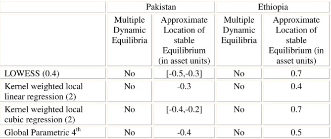
Table 1 reports the results of the estimation techniques introduced in section 6. All techniques find only a single dynamic asset equilibrium for rural households in Pakistan and Ethiopia. The different methods also agree to a great extent where this asset

equilibrium is located. Thus, the method of estimation does not seem to matter in identifying asset equilibria, at least not when the asset dynamic path is a very smooth concave function, as in the two datasets used.

Table 1 Asset Equilibria Estimates of all Techniques

Pakistan Ethiopia Multiple Dynamic Equilibria Approximate Location of stable Equilibrium (in asset units)

Multiple Dynamic Equilibria Approximate Location of stable Equilibrium (in asset units) LOWESS (0.4) No [-0.5,-0.3] No 0.7

Kernel weighted local

linear regression (2) No -0.3 No 0.4

Kernel weighted local

cubic regression (2) No [-0.4,-0.2] No 0.7

order Polynomial

Median Cubic Spline No -0.6 No 0.4

Natural Cubic Spline No [-0.5, -0.2] No 0.8

Nonparametric Penalized

Spline No -0.4 No 0.6

Semiparametric Penalized

Spline No -0.4 No 0

Bandwidth in parentheses.

The long run equilibrium levels are very low in both countries. Since the asset index was constructed to have mean zero, the long run asset equilibrium in Pakistan of around -0.4 asset units is even below the mean. The Ethiopian equilibrium at 0.5 asset units is only just above the mean. Considering that both surveys intentionally sampled poor regions, this means that the asset equilibria are very low indeed.

LOWESS and kernel weighted local linear and polynomial regression estimates were unaffected over a large range of bandwidths. This is unsurprising given the smooth nature of the asset recursion function.

Asset recursion diagrams for the nonparametric penalized spline regressions (see

Equation 3)12 _{are shown in Graph 6 and Graph 7. Both show clearly the single equilibria,}

the dynamic asset accumulation path and its 95 percent confidence band. The rug plot at the bottom of the graphs displays the distribution of the observations.

12_{Estimated using the R command ‘spm’ (Wand, et al., 2005) using default knot locations (} 1

2

k k

K

κ= +₊ th

Graph 6 Pakistan Assets vs. Lagged Assets (Nonparametric Estimation by Penalized Splines) -2 -1 0 1 2 -1 .5 -1 .0 -0 .5 0. 0 0. 5 1. 0 Asset.lag A ss et

Graph 7 Ethiopia Assets vs. Lagged Assets (Nonparametric Estimation by Penalized Splines)

-2 -1 0 1 2 -2 -1 0 1 2 Asset.lag A ss et

All the other nonparametric techniques led to substantively similar recursion diagrams, which are therefore not shown. The degrees of freedom used by the penalized spline in fitting the nonparametric function f(Ait-1) are an indication of the nonlinearity of the asset

is more than the 2.7 used for the Ethiopian estimation, but is still fairly small. This

implies that both countries’ dynamic asset accumulation paths are not very nonlinear. The larger degree of concavity and the greater distance from the diagonal of the Pakistani function indicate that households move along the asset accumulation path more quickly than those in Ethiopia.

The penalized spline estimations are robust to changes in the specification. Using truncated polynomial spline bases linearly or quadratically instead of cubic thin plate spline bases did not affect the result; neither did a relatively large change in the smoothing parameter . To let the penalized spline follow the data more closely I

specified 20 degrees of freedom compared to the 4 corresponding to the REML choice of smoothing parameter.

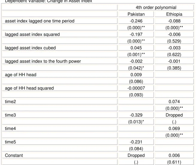
The global polynomial parametric regression results are reported in Table 2. In the Pakistan data there are life cycle effects in asset holdings. The coefficient for the age of the household head is positive, whereas that for the squared age is negative. Asset holdings increase at a decreasing rate up to a maximum at age 40 before falling again.

Table 2 Global Polynomial Regressions (Random Effects)

Dependent Variable: Change in Asset Index

4th order polynomial

Pakistan Ethiopia

asset index lagged one time period -0.246 -0.088

(0.000)** (0.000)**

lagged asset index squared -0.197 -0.006

(0.000)** (0.529)

lagged asset index cubed 0.045 -0.003

(0.001)** (0.622)

lagged asset index to the fourth power -0.002 -0.001

(0.042)* (0.385)

age of HH head 0.009

(0.086)

age of HH head squared -0.00007

(0.093) time2 0.074 (0.000)** time3 -0.329 Dropped (0.013)* (.) time4 0.069 (0.000)** time5 -0.231 (0.084) Constant Dropped 0.006 (.) (0.611)

Observations 1384 4036

Number of Households 722 1369

p values in parentheses

* significant at 5%; ** significant at 1%

Time 1 is the excluded time dummy in both models.

To translate the regression coefficients of the lagged asset variables into the asset recursion diagram I predicted the dependent variable ‘change in asset index’, and then subtracted the lagged asset index. This gives the predicted asset index, which is plotted against the lagged index as the inner red line in Graph 8 and Graph 9. The outer green lines show the 95% confidence bands. Results for third order polynomial estimates are almost identical.

Graph 8 Pakistan Assets vs. Lagged Assets (4th order Global Parametric Estimation)

-1

-.5

0

.5

-1 -.5 0 .5

assethat/asset index lagged one time period

Graph 9 Ethiopia Assets vs. Lagged Assets (4th _{order Global Parametric Estimation)}

-1 0 1 2 th at /lo w es s as se th at a ss et _l ag /lo w es s hi gh a ss et _l ag /lo w es s lo w a ss et _l ag -1 0 1 2

The simple semiparametric partial linear model estimations for Equation 6 are shown for Pakistan and Ethiopia in Graph 10 and Graph 11.

For Pakistan the non-linear components uses 3 degrees of freedom. The location of the asset equilibrium is unchanged at around -0.5, but the curve starts to bend back at higher asset levels. However, this result is driven by very few observations at the top of the distribution.

The Ethiopian recursion diagram is again slightly more linear than the one for Pakistan, using only 1.6 degrees of freedom. However, the semiparametric estimation for Ethiopia does affect the location of the asset equilibrium, moving it to around 0 asset units. To further explore whether the semiparametric specification makes a substantive difference I intended to also estimate the semiparametric mixed model from Equation 7 which also controls for household effects. However, the R maximization algorithm has so far always crashed.

Graph 10 Pakistan Semiparametric Estimation of Assets vs. Asset Lagged (Penalized Splines)

0 2 4 6 8 0 2 4 6 8 10 Asset.lag A ss et

Graph 11 Ethiopia Semiparametric Estimation of Assets vs. Asset Lagged (Penalized Splines) -2 -1 0 1 2 3 -2 -1 0 1 2 Asset.lag A ss et

Finally, I tested the robustness of the above results against two alternative explanations of why we only see one asset equilibrium.

First, social sharing rules may mean that any gains in assets by one household are at least partly distributed to its social networks. Alternatively, household composition may be endogenous. If a household manages to accumulate assets it also attracts people currently living outside of it to join the household. Both of these mechanisms would mean that a household above the dynamic equilibrium moves back to it over time. A way to test for these alternative explanations is to re-estimate the livelihoods function in Equation 1 but using household consumption rather than household consumption adjusted by household subsistence needs as the dependent variable. The asset index would then reflect any additional assets gained by the household, whether or not their returns were consumed by the (original) household members. Rerunning the different estimation techniques on this new asset index revealed that the results did not change, suggesting that social sharing rules and endogenous household composition don't explain the observed pattern.

A second reason why we might not see multiple equilibria is that the time period between observations is short. If total asset holdings change slowly, the short spell panels may not pick up the long run dynamics. In the ERHS sample three spells are only five months long, and the last one is two years. In the PRHS sample used observations are only two years apart. In contrast, the studies which have found multiple asset equilibria have either used longer spells - the South African (Adato, et al., forthcoming) and the Western Kenyan panel (Barrett, et al., 2004) span five and thirteen years, respectively – or are based only on pastoralists’ livestock holdings, which are much more volatile than other

asset holdings (see the studies on Northern Kenyan (Barrett, et al., 2004) in or Southern Ethiopian (Lybbert, et al., 2004)).

To test this explanation I constructed the longest possible spells for both surveys – three years for Ethiopia, and five for Pakistan – and reran the above nonparametric estimations. These results are not reported here, but are virtually identical. Thus, it seems safe to conclude that the data do indeed display concave asset accumulation paths and do not have multiple equilibria.

Finally there are two other possible, but untestable, explanations as to why the data do not show bifurcating welfare dynamics. First, a qualitative survey from Ethiopia has shown that bifurcating equilibrium paths may depend on the quality of the growing season. When years are good all farmers expect to be on concave accumulation path. In contrast, in mediocre years only some farmers, including probably the experienced, expect to grow, whereas others expect to fall behind (Santos and Barrett, 2005). This may be an explanation for the concave pattern in Ethiopia as the ERHS rounds fell into

relatively good years.

Second, the survey designs explicitly cover poor populations. It is possible that in the countries as a whole there are additional higher asset equilibria13, which the surveys miss as they simply did not capture these richer areas or households. The only way to test for this would be to use a nationally representative panel survey. If indeed, there are higher equilibria in other rural or urban parts of the country, then the findings in this paper could be interpreted as geographic poverty traps.

8 Conclusions

This paper tested previously used nonparametric and parametric techniques to identify asset poverty dynamics and asset thresholds in two countries. It also adapted different, semiparametric estimation methods to combine the advantages of flexible functional form and control for household and time specific effects.

All econometric methods concur that the process of asset accumulation for rural Pakistani and Ethiopian households is linear. However, there is no evidence for

non-convexities in asset dynamics, which would be necessary for multiple stable asset equilibria. This would imply that households in rural Pakistan and Ethiopia do not face asset poverty traps, but instead would be expected to gravitate towards one long run equilibrium. By implication, no households would suffer permanently from short term asset shocks, but would recover over time. These conclusions do not come as a surprise given the single peaked nature of empirical distribution of the asset index.

The non-linearity that I do find is a (slightly) concave pattern of asset accumulation, more so in Pakistan than in Ethiopia. The concave recursion diagrams imply that the speed of

asset accumulation is a positive function of the initial level of asset holdings. Initially asset-poor households accumulate assets more slowly than those households which have more assets, but are still below the (single) long run equilibrium. This mirrors the findings for Russia and Hungary in Lokshin and Ravallion (2001) and for rural China in Jalan and Ravallion (2001). As a corollary, concavity further suggests that poorer households recover from asset shocks more slowly than richer households. In the presence of frequent shocks the slow speed of adjustment could mean that poor households never reach the single long run equilibrium.

From a practical policy point of view, finding a single asset equilibrium – even regardless of where it is located – does not imply that there is no need to provide assistance to asset poor households to help them escape poverty. It is quite possible that progress towards the one long run equilibrium is so slow that it would take unacceptably long for very poor households to reach.

The concave asset recursion diagram also supports the case for redistribution of assets, as it suggests that reducing asset inequality could enhance subsequent growth.

A key issue for policy purposes is how to interpret the equilibrium asset index values. Any policy recommendation would of course need to know how the index translates back into asset themselves. We can of course work back mechanically and use the scoring coefficients from the factor analysis to ‘recover’ typical asset levels associated with the one asset equilibrium. That would give the average value of all the assets in the index that a household would have in equilibrium, thus creating a ‘representative household’. This concept, however, has limited value, as any number of linear combination of factors can yield that same asset index, not just the combination of ‘average’ assets.

Moreover, there may be economies of scale and of scope in reaching the equilibrium level of assets (and well-being). That is, there is likely to be limited substitutability, and a considerable degree of complementarity between assets. This makes it difficult to identify which particular assets households below the equilibrium need assistance with; let alone identifying which particular combination of assets is required. There is a need to

disentangle the effects of different assets. This can be done in two different ways. Either by supplementing quantitative surveys with qualitative data, where particular types of households identified from the quantitative data are revisited and asked further questions about their gains and losses of assets (Adato, et al., forthcoming), or potentially using other statistical techniques which do not rely on an asset index, but still enable flexible modeling of individual assets and interactions of assets. Additive models and single index models are potential candidates. In terms of modeling asset dynamics using an asset index, the random effects semiparametric mixed model probably represents the best available technique.

Of course, we would also like to relate the dynamic equilibrium asset index levels to a poverty line, defined in assets and preferably also in income/expenditure. The estimated long run equilibria alone do not tell us whether a household at the equilibrium level has escaped poverty. Again the many different asset combinations which can add up to the

same overall asset index make it difficult to relate the asset equilibrium to a unique level of consumption.

In addition to being robust across econometric specifications the results in this paper are also robust to different ways of constructing the asset index, whether by factor analysis or livelihood regressions. Results are also unaffected by whether the asset index is

constructed using household or adult equivalent level variables, and by different lengths of asset spells. This could well be a reflection of the relatively linear dynamic asset accumulation path.

The only slightly nonlinear nature of the recursion diagrams also suggests that the Pakistan and Ethiopia datasets may not be the most suitable for a paper that tries to compare existing and apply new methods in testing for multiple dynamic equilibria! A priori we would expect that the smoother the dynamic asset path is , the less the estimation technique matters. In other words, the more linear the path, the less we are going to add by using nonlinear methods. The strong concurrence of results for rural Pakistan and Ethiopia reflect that in practice.

However, asset accumulation paths don’t have to be this smooth, as seen by the results in Adato et a. (forthcoming) and Barrett et al. (2004). In such cases choice of estimation technique is likely to matter more, both in terms of identifying the existence of multiple equilibria as well as their location. A next step would be to apply the estimation

techniques from this paper to nationally representative panel surveys, in which households would be less homogenous than in rural-only surveys, and to surveys in which multiple asset equilibria have been found by previous studies.

References

Adato, M., M. R. Carter, and J. May. "Sense in sociability? Social exclusion and persistent poverty in South Africa." Journal of Development Studies

(forthcoming).

Aghion, P., E. Caroli, and C. Garcia-Penalosa. "Inequality and economic growth: The perspectives of the the New Growth Theories." Journal of Economic Literature

37, no. 4(1999): 1615-1660.

Azevedo, J. P. W. (undated) Factortest STATA ado file.

Banerjee, A., and E. Duflo. "Inequality and Growth: What can the data say?" Journal of

Economic Growth 8(2003): 267-299.

Banerjee, A., and A. Newman. "Occupational choice and the process of development."

Journal of Political Economy 101(1993): 274-298.

Barrett, C. B. "Rural Poverty Dynamics: Development Policy Implications." Agricultural Economics (forthcoming).

Barrett, C. B., et al. "Welfare dynamics in rural Kenya and Madagascar." Cornell University.

Barrett, C. B., and J. G. McPeak (forthcoming) Poverty traps and safety nets, ed. A. de Janvry, and R. Kanbur. Amsterdam, Kluwer.

Basu, K. "Child Labor: Cause, Consequence and Cure with remarks on International Labor Standards." Journal of Economic Literature 37, no. 3(1999): 1083-1119. Carter, M. R., and C. B. Barrett. "The economics of poverty traps and persistent poverty:

An asset-based approach." Journal of Development Studies (forthcoming). Carter, M. R., and J. May. "One Kind of Freedom: Poverty Dynamics in Post-apartheid

South Africa." World Development 29, no. 12(2001): 1987-2006. Dasgupta, P., and D. Ray. "Inequality as a determinant of malnutrition and

unemployment theory." Economic Journal 96(1986): 1011-1034.

de Boor, C. A Practical Guide to Splines. 2nd Edition ed. New York: Springer, 2002. Emerson, P., and A. Souza. "Is there a child labor trap? Intergenerational persistence of

child labor in Brazil." Economic Development and Cultural Change 51, no. 2(2003): 375-398.

French, J. L., E. E. Kammann, and M. P. Wand. "Comment on paper by Ke and Wang."

Journal of the American Statistical Association 96(2001): 1285-1288.

Galor, O., and J. Zeira. "Income distribution and macroeconomics." Review of Economic Studies 60, no. 1(1993): 35-62.

Hastie, T., R. Tibshirani, and J. Friedman. The elements of statistical learning: Data mining, inference, and prediction. Springer Series in Statistics. New York: Springer Verlag, 2001.

Jalan, J., and M. Ravallion. Household Income Dynamics in Rural China. World Bank Policy Research Working Paper 2706. Washington, DC: World Bank, 2001. Lokshin, M., and M. Ravallion. "Household Dynamics in Two Transition Economies."

Studies in Nonlinear Dynamics & Econometrics 8, no. 3(2001).

Lybbert, T., et al. "Stochastic wealth dynamics and risk management among a poor population." Economic Journal 114(2004): 750-777.

Mirrlees, J. (1975) A pure theory of underdeveloped economies, ed. L. Reynolds. New Haven, Yale University Press.

Pagan, A., and A. Ullah. Nonparametric Econometrics. Cambridge: Cambridge University Press, 1999.

Ruppert, D. "Selecting the number of knots for penalized splines." Journal of Computational and Graphical Statistics 11(2002): 735-757.

Ruppert, D., M. P. Wand, and R. J. Carroll. Semiparametric Regression. Cambridge Series in Statistical and Probabilistic Mathematics. Cambridge: Cambridge University Press, 2003.

Sahn, D., and D. Stifel. "Poverty comparisons over time and across countries in Africa."

World Development 28, no. 12(2000): 2123-2155.

Santos, P., and C. B. Barrett. "Social Safety Nets or Insurance in the Presence of Poverty Traps." Cornell University.

Schumaker, L. Spline Functions: Basic Theory. New York: Wiley and Sons, 1981. Stiglitz, J. E. "The efficiency wage hypothesis, surplus labor and the distribution of

income in LDCs." Oxford Economic Papers 28(1976): 185-207. Wand, M. P., et al. (2005) SemiPar 1.0. R package. http://cran.r-project.org.

Appendix A Summary Statistics of Datasets

Summary statistics Pakistan Rural Household Survey

Variable Obs Mean Std. Dev. Min Max

HH COMPOSITION

# of HH members of working age 2440 0.696 0.214 0.211 1.266

# of children 2440 0.517 0.265 0 1.109

EDUCATION

# of illiterate HH members 2440 0.215 0.214 0 1.258

# of HH members with some primary

education 2440 0.013 0.052 0 0.643

# of HH members with primary school 2440 0.027 0.059 0 0.560 # of HH members with middle school 2440 0.013 0.040 0 0.465 # of HH members with secondary

school 2440 0.015 0.046 0 0.629

# of HH members with college 2440 0.008 0.034 0 0.520 LAND

Land owned (acres) 2429 1.449 5.471 0 108

Irrigated land owned (acres) 2429 0.540 1.359 0 13.158

Land operated (acres) 2429 0.951 1.550 0 32.258

Irrigated land operated (acres) 2429 0.605 1.071 0 10.397 OTHER ASSETS

Livestock (TLUs) 2066 0.529 0.443 0 4.842

Value of agricultural assets 2285 39466 329553 0 10800000

Value of tools 1973 1.233 1.764 0 59.766

Total value of all houses owned 2305 8757 15176 0 168919 Total value of durables owned 2305 2767 7850 0 194976 FINANCIAL

Rs. Paid into any accont 2304 540 5139 0 218447

Rs. Taken out of any account 2304 280 4613 0 212379

Total amount of loans received 2302 2764 7201 0 148716

Real Income per capita 2185 3900 4834 0 118819

ASSET INDEX

Asset index 2157 0.000 0.822 -0.9243 13.21

Asset index lagged one period 1408 0.047 0.809 -0.9243 8.18 Change in asset index 1383 -0.122 0.507 -4.9044 5.55 Note: All variables are in per capita terms.

Summary Statistics Ethiopia Rural Household Survey

Variable Obs Mean Std. Dev. Min Max

Household Size 5856 4.70 2.387 0.125 32.94

Consumption 5726 100.48 115.07 1.262 3584

# of able bodied adults 5856 0.478 0.365 0 6.75

Total Education 5856 0.426 0.674 0 16.96

Value of Farm tools 5519 22.32 47.797 0 999.3

Livestock (TLUs) 5607 .69 0.938 0 14.14

Asset Index 5445 -2.51e-10 0.829 -2.39 6.76

Lagged Asset Index 4081 -.021 0.842 -2.39 6.76

Change in Asset Index 4036 0.045 0.426 -3.95 3.76