NBER WORKING PAPER SERIES
TWO TREES: ASSET PRICE DYNAMICS
INDUCED BY MARKET CLEARING
John H. Cochrane
Francis A. Longstaff
Pedro Santa-Clara
Working Paper
10116
http://www.nber.org/papers/w10116
NATIONAL BUREAU OF ECONOMIC RESEARCH
1050 Massachusetts Avenue
Cambridge, MA 02138
November 2003
John Cochrane gratefully acknowledges research support from an NSF grant administered by the NBER and from the CRSP. We are grateful for the comments and suggestions of Michael Brandt, George Constantinides, Vito Gala, Lars Peter Hansen, John Heaton, Jun Liu, Monika Piazzesi, Rene Stulz, Pietro Veronesi, and seminar participants at the University of Chicago. We are also grateful to Bruno Miranda for research assistance. All errors are our responsibility.The views expressed herein are those of the authors and not necessarily those of the National Bureau of Economic Research.
©2003 by John H. Cochrane, Francis A. Longstaff, and Pedro Santa-Clara. All rights reserved. Short sections of text, not to exceed two paragraphs, may be quoted without explicit permission provided that full credit, including © notice, is given to the source.
Two Trees: Asset Price Dynamics Induced by Market Clearing
John H. Cochrane, Francis A. Longstaff, and Pedro Santa-Clara
NBER Working Paper No. 10116
November 2003
JEL No. J3, O3
ABSTRACT
If stocks go up, investors may want to rebalance their portfolios. But investors cannot all rebalance.
Expected returns may need to change so that the average investor is still happy to hold the market
portfolio despite its changed composition. In this way, simple market clearing can give rise to
complex asset market dynamics. We study this phenomenon in a very simple model. Our model has
two “Lucas trees.” Each tree has i.i.d.dividend growth, and the representative investor has log utility.
We are able to give analytical solutions to the model. Despite this simple setup, price-dividend
ratios, expected returns, and return variances vary through time. A dividend shock leads to
“underreaction” in some states, as expected returns rise and prices slowly adjust, and “overreaction”
in others. Expected returns and excess returns are predictable by price-dividend ratios in the time
series and in the cross section, roughly matching value e.ects and return forecasting regressions.
Returns generally display positive serial correlation and negative cross-serial correlation, leading
to “momentum,” but the opposite signs are possible as well. A shock to one asset’s dividend a.ects
the price and expected return of the other asset, leading to substantial correlation of returns even
when there is no correlation of cash flows and giving the appearance of “contagion.” Market
clearing allows the “inverse portfolio” problem to be solved, in which the weights of the assets in
the market portfolio are “inverted” to solve for the parameters of the assets’ return generating
process.
John H. Cochrane
Graduate School of Business
University of Chicago
1101 E. 58
thStreet
Chicago, IL 60637
and NBER
[email protected]Francis A. Longstaff
The Anderson School at UCLA
P.O. Box 951481
Los Angeles, CA 90095-1481
and NBER
Pedro Santa-Clara
The Anderson School at UCLA
P.O. Box 951481
1. INTRODUCTION
When stocks do better than bonds, growth stocks do better than value stocks, or the Nasdaq does better than the S&P 500, there is much talk about rebalancing portfolios. But everyone cannot rebalance. Expected returns must adjust, or other moments must change, so that the average investor is still happy to hold the market portfolio, despite its larger weight in the asset that has gone up. In this way, the market-clearing condition can induce dynamics in stock prices and returns, even when the underlying preferences are stable and the underlying cashflows are i.i.d.
To characterize dynamics induced by market clearing, we examine a simple model withtwo“Lucas trees.” Each tree gives a dividend stream that follows a geometric Brownian motion. The representative investor has log utility and consumes the sum of the trees’ dividends. We obtain explicit closed-form solutions for prices and expected returns.
With one tree, of course, this model leads to a constant price-dividend ratio, a constant interest rate, and i.i.d. returns. With two trees, price and return dynamics emerge. Aggregate consumption diversifies across the two trees, so it is more volatile when dividend shares are near zero or one than when the shares are more equal. This time-varying volatility of consumption growth, and therefore of the discount factor, generates time-varying expected returns and volatility for the market, the individual assets, and a time-varying riskless rate.
Why is this new? In traditional finance models such as the CAPM or ICAPM, the rate of re-turn is exogenous and independent of the scale of investment. These models implicitly assume linear technologies — output is a linear function of capital — with no adjustment costs or irreversibilities. In these models, wecan all rebalance, by instantly and costlessly transferring capital to other production technologies or to consumption; wecanall leave portfolio weights constant in the face of return shocks. In reality, however, market portfolio weights do change over time (e.g. stocks vs. bonds). Thus, any realistic model, with at least short-run adjustment costs, irreversibilities, and other impediments to aggregate rebalancing, will contain some market-clearing induced dynamics of the sort we isolate and study in a pure exchange economy.
The asset price and return dynamics of the two-tree model are similar to those found in the empirical asset pricing literature. First, wefind that a positive dividend shock, which increases current prices and returns, also typically raises subsequent expected returns and excess returns, as the intuition of thefirst paragraph suggests. Thus, returns typically display positive autocorrelation or “momentum,” prices typically seem to “underreact” or not to “fully adjust” to dividend news, and to “drift” upwards for some time after that news. Interestingly, however, there are also parameters, horizons, and regions of the state space that give the opposite signs, leading to “mean-reversion,” price “overreaction,” and “downward drift,” such as that found after IPOs, and “excess volatility” of prices and returns.
Second, when one asset has a positive dividend shock, the expected return of the other asset typically declines. We see a negative cross-serial correlation, which Lo and MacKinlay (1990) and Lewellen (2002) argue is an important part of the momentum effect. We see movements in an asset’s price even with no news about that asset’s dividends, another source and form of apparent “excess volatility.” Finally, we see that asset returns can be highly correlated with each other even when their
underlying dividends are independent. A “common factor” or “contagion” emerges in returns even though there is no common factor in cashflows.
Third, since price-dividend ratios vary despite i.i.d. dividend growth, price-dividend ratios forecast returns in the time series and in the cross section, i.e. we see value and growth effects. Thus, simple market-clearing mechanics generate simultaneously short-run momentum (positive autocorrelation) and long-run mean reversion (valuation ratios forecast returns) in individual stocks and in the stock market as a whole.
While these asset price and return dynamics are qualitatively similar to the stylized facts of the empirical literature, our two-tree log utility model does not typically offer aquantitatively compelling match. In our informal calibration, typical statistics such as autocorrelations are between a factor of two and an order of magnitude smaller than their counterparts in the empirical literature. Any log utility model will of course not match the large mean and volatility of returns with the low volatility of aggregate consumption and dividend growth. Also, none of our dynamic effects are pricing puzzles, as all expected returns are explained by the consumption-based model or the CAPM in a log utility model. (The CAPM in our model does require properly measured conditional betas, a time-varying market premium, and use of the entire consumption claim as a reference return rather than just the stock portfolio. Puzzles would still be generated by the failure to incorporate any of these side conditions.)
The point of this paper, however, is not to provide a quantitatively convincing match to a wide range of asset pricing puzzles. Rather, it is to show how market-clearing logic, a heretofore ignored source of asset pricing dynamics, can produce interesting dynamics even in a very stylized model — two geometric Brownian trees and log utility. This mechanism will be an important part of more complex and realistic (but also less transparent) models. Put another way, the one-tree model with log utility is a workhorse, despite its obvious unrealism, since it is simple to solve and it illustrates so many of the economic principles that underlie more quantitatively realistic models. Our two-tree model fills a similar niche. Many of its predictions, while matching the signs reported in the empirical literature, do not match the magnitudes. Yet it is a simple, tractable model with closed-form solutions, which captures and clearly displays interesting economic effects which will also be present in more complex models.
Market clearing has not played a central role in traditional dynamic models of asset pricing. Models with exchange economies typically assume a single asset in nonzero supply (Lucas (1978)). Production economies sidestep the issue by allowing the supply of assets to change elastically with investor demand (Cox, Ingersoll, and Ross (1985)). However, a recent literature examines and prices multiple long-lived dividend streams in nonzero net supply, generalizing standard single-tree models. Santos and Veronesi (2001), Bansal, Dittmar, and Lundblat (2002), and Menzly, Santos, and Veronesi (2003) offer Lucas-type models with multiple assets. Their models have interesting dynamics for dividend shares, interesting preferences (e.g. habits), and they are designed to address quantitatively a variety of stylized facts.
The paper closest to ours is Santos and Veronesi (2001). They specify log utility and two “trees,” which they interpret as assets and labor income. Like ours, their model predicts that expected returns, price-dividend ratios, betas, and so forth should vary as functions of the dividend share. They reproduce and extend a number of empirical facts involving asset price dynamics. In particular, they show how the share of labor income in total consumption performs well in forecasting stock returns. The main difference is that they specify the share process to be mean reverting, which exogenously builds dynamics into the dividend processes. This ingredient is potentially an additional source of asset price dynamics. We focus on a model with a simpler ingredient, i.i.d. dividend growth, in order to focus on the question: what dynamics come from the simple logic of market clearingalone?
enables the solution of theinverse portfolio-choice problem. In the usual portfolio-choice problem, we are given the return process and then solve for the optimal portfolio. In theinverse portfolio-choice problem, we are given the optimal portfolio and then solve for the moments of returns that support those holdings. We verify that the solution to theinverseportfolio-choice problem gives the same results as our endowment economy calculations.1
The conundrum that we cannot all rebalance, so returns cannot in general be i.i.d. shows up several places infinance. Rosenberg and Ohlson (1976) and Cheng and Grauer (1980) note that relative prices and returns cannot vary ex-post if one pairs the CAPM with constant share supply.
2. THE SINGLE-ASSET BENCHMARK
To provide a benchmark for comparison, we begin by reviewing the traditional single-asset model. The asset pays a dividend stream
dD
D = µ dt + σdZ, (1)
with constant coefficientsµ andσ, and whereZ is a standard Brownian motion. Unless necessary for clarity, we suppress time indices, e.g. dD≡dDt, etc. The representative investor has log utility,
Ut = Et
∞ 0
e−δτ ln (Ct+τ) dτ . (2)
This is an endowment economy, so prices adjust until consumption equals the dividend,C =D. The investor’sfirst-order condition implies that marginal utility is a discount factor that prices assets,
Mt=e−
δt
Dt
. (3)
The pricePt of the asset, which is the “market portfolio” claim to aggregate consumption, is given by
Pt Ct = 1 Dt Et ∞ 0 Mt+τ Mt Dt+τ dτ = Et ∞ 0 e−δτ Dt+τ Dt+τ dτ = 1 δ. (4)
Since prices are proportional to consumption (which equals the dividend), price appreciation is the same as dividend growth, dP P = dC C = dD D , (5)
1Black and Litterman (1990) use the market-clearing condition to back out expected returns from
knowledge of the covariance matrix and the market capitalization weights of the different assets. He and Leland (1993) impose a market-clearing condition to derive dynamics of asset prices that are consistent with equilibrium.
so that the total instantaneous returnRtis
Rt = dPt
Pt +
Dt
Pt dt = (µ + δ)dt + σdZ. (6)
The expected return and return variance are constant,
Et[Rt] = (µ + δ)dt, (7)
Vart[Rt] = σ2 dt. (8)
Thus, dividend growth rates and stock returns are i.i.d. through time in this single-asset model. The instantaneous interest rate is given by
r dt = −Et dMt Mt = δdt + Et dDt Dt − Vart dDt Dt = (δ + µ − σ2)dt. (9)
The riskless asset is in zero net supply. We see the standard discount rate (δ), consumption growth (µ), and precautionary savings (σ2) effects. Since the riskless rate is constant, the entire term structure is
constant andflat.
3. THE TWO-ASSET MODEL
Now consider the same economy with two assets but no other modifications. As before, dividends follow simple geometric Brownian motions,
dDi
Di =µi dt + σi dZi, (10)
wherei= 1,2, and the correlation betweendZ1 anddZ2 isρdt. Aggregate consumption is the sum of
the two dividendsC=D1+D2. The investor has log utility as in Equation (2).
The dividend share,
s= D1
D1+D2
, (11)
is a natural state variable for the two-tree model. Wefirst derive the dynamics of the dividend share. We thenfind the interest rate and price the market portfolio from the aggregate consumption process. Finally, we price the individual assets andfind returns, expected returns, and variances of returns.
3.1 Dividend Share Dynamics.
An application of Itˆo’s Lemma to Equations (10) and (11) gives the dynamics of the dividend share,2
ds=s(1−s) µ1−µ2−sσ12+ (1−s)σ22+ (2s−1)ρσ1σ2 dt+s(1−s)(σ1 dZ1−σ2dZ2). (12)
The drift of the dividend share process in (12) is zero whens= 0,κ,or 1, where
κ= µ1−µ2+σ 2 2−ρσ1σ2 σ2 1+σ22−2ρσ1σ2 . (13)
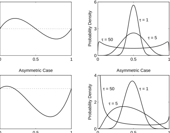
Whenκlies between zero and one, the drift is positive from zero toκ, bringing the share up towardsκ, and negative fromκto one, bringing the share down towardsκ. The top left panel of Figure 1 illustrates the drift process for a case in which dividend dynamics are symmetric; the bottom left panel of Figure 1 illustrates the drift process for a case in which the dividends for thefirst asset are more volatile than for the second asset. Thus, the drift term can induce patterns of mean reversion in the dividend share that are not present in the underlying dividend processes.3 The diffusion coefficient in Equation (12) is
quadratic, implying that changes in the dividend share are most volatile whens= 1/2. Initially, it may seem surprising that simple geometric Brownian dividends give rise to a complex share process with a cubic drift and a quadratic diffusion. However, these properties of share dynamics result directly from the nonlinearity of the share as a function of the dividends.
The density f(sτ | s) of the dividend share τ periods ahead conditional on its current values is given by4 f(sτ|s) = 1 sτ(1−sτ) 2πη2τ exp −[ln (s/(1−s))−ln (sτ/(1−sτ))−ντ] 2 2η2τ , (14) where
2The stochastic process for the sharesis a member of the important class of Wright-Fisher diffusions.
In an interesting parallel to our two-asset model, these types of diffusions are often applied in genetic theory to characterize the evolution of genes in a population of two genetic types. For example, Karlin and Taylor (1981) Ch. 15, p. 184-188 present an example of the Wright-Fisher gene frequency diffusion model in which the fraction of genes in a population follows a process with drift and diffusion terms that are respectively third- and second-order polynomials in the fraction, just as in Equation (12). Also see Crow and Kimura (1970) for other examples and a discussion of the asymptotic properties of these models.
3The cubic drift of our share process is also closely related to that of the stochastic Ginzburg-Landau
diffusion used in superconductivity physics to model phase transitions. See Kloeden and Platen (1992) and Katsoulakis and Kho (2001).
4Rather than solve the Kolmogorov or Fokker-Planck equation associated with Equation (12) directly,
we express the share as an invertible function of the lognormally distributed ratio D1/D2, i.e. s =
(1 +D2/D1)−1. Since the ratio of lognormals is lognormal, we then solve for the density using a
ν=µ2−µ1−σ22/2 +σ12/2, η2=σ12+σ22−2ρσ1σ2.
Note thatν dt=E[dln(D2/D1)] andη2dt= Var[dln(D2/D1)]. The mean and variance of log dividend growth drive the distribution. Although the underlying dividends are lognormal, the dividend share itself is not lognormal. From Equation (14), one can verify analytically that the distribution of sτ can be either unimodal or bimodal, and can display either positive or negative skewness. As one might expect of the share formed from two geometric Brownian motions, the dividend share is strictly between zero and one for allfinite horizons, provided current dividends are nonzero. An increase in the current dividend share shifts the distribution ofsτ towards larger values for allfiniteτ.
The right hand panels of Figure 1 plot the conditional density of the dividend share given in Equation (14) for several horizons. In the top right panel, the dividend dynamics are symmetric and the initial dividend share equals 50 percent. In this case, the distribution of the dividend share is initially unimodal, but eventually spreads out and begins to look more uniformly distributed. After 50 years, the distribution becomes bimodal as the probability of being in the neighborhoods of zero and one slowly increases.
The bottom right panel of Figure 1 shows densities for an asymmetric case in which thefirst asset has a higher volatility than the second and the initial dividend share is 20 percent. Here, the distribution of the dividend share becomes skewed toward the right, and large values for the dividend share become more likely. The larger volatility of the smaller dividend process gives it some chance of overtaking the initially larger dividend process. As the horizon increases further, however, the distribution tends to shift back towards smaller values.
The dividend share is both persistent and volatile for the parameter values we examine. The conditional mean share does not move quickly over time, as seen both in the small values of the drifts (top panel of Figure 1) and in the means of the densities (middle and bottom panels of Figure 1). This is persistence. However, the densities in Figure 1 spread out rapidly, so changes in the share are very volatile.
This model does not possess a stationary share distribution. The share of one of the assets will al-ways gradually decline to the point that the other asset becomes dominant in the market.5A degenerate long-run share distribution may seem counterintuitive, but it is not necessarily an unrealistic feature of the model. First, it may be hard to tell. Given realistic parameter values, the mean time until the share of onefirm is less than, say,five or ten percent of its initial value may be on the order of centuries. Thus, this aspect of the cashflow stream may have little effect on its present value. Second, firms do in fact disappear over long periods of time. As one recent example, Fama and French (2003)find that more than 15 percent of seasonedfirms are delisted from the stock market for poor performance during a typical decade. The right generalization may be to allow the birth of new trees, not to preclude the death of old trees.
3.2 Consumption Dynamics.
Aggregate consumptionC=D1+D2 follows
5This feature parallels the asymptotic properties of Wright-Fisher gene frequency models in which one
dC = dD1 + dD2,
= µ1D1dt + µ2D2 dt + σ1D1dZ1 + σ2D2 dZ2, (15)
so that
dC
C = µ1s + µ2(1−s) dt + σ1s dZ1 + σ2(1−s)dZ2. (16)
Since the dynamics of consumption depend on the state variable s, consumption growth is no longer i.i.d. through time. Mean consumption growth,
Et
dC
C = [µ1s+µ2(1−s)]dt, (17)
is the share-weighted mean of the dividend growth rates. Consumption volatility,
Vart dC
C = [σ
2
1s2+σ22(1−s)2+ 2ρσ1σ2s(1−s)]dt, (18)
is lower for intermediate values of the dividend share, as consumption is then diversified between the two dividends.
3.3 The Riskless Rate.
Wefind the instantaneous (zero net supply) interest rate as before
r dt = δdt + Et dC
C − Vart
dC
C . (19)
Substituting the moments of the consumption dynamics into Equation (19) gives
r = δ + µ1s + µ2(1−s) − σ21s2 − σ22(1−s)2 − 2ρσ1σ2s(1−s). (20)
Thus, the riskless rate varies over time, as a quadratic function of the state variables. The riskless rate is lower for intermediate values of the dividend share because dividend diversification lowers consumption volatility, which lowers the precautionary savings motive. Since the interest rate is not constant, the term structure is notflat.
3.4 Market Price and Returns.
As is usual in log utility models, the pricePm of the aggregate consumption streamC=D1+D2 (the market portfolio) is given by the simple expression
Pmt Ct = Et ∞ 0 e−δt Ct+τ Ct+τ dτ = 1 δ. (21)
This calculation, which is the same as in the single-asset model, is valid for all consumption dynamics. Since aggregate consumption equals aggregate dividends, Equation (21) also implies that the market price-dividend ratio is constant. As before, the price of the market is proportional to aggregate con-sumption which implies that the price appreciation of the market is
dPm
Pm =
dC
C . (22)
Since the total instantaneous returnRM on the market equals price appreciation plus the dividend yield (Rm= dPm Pm + C Pmdt= dC C +δdt), Equation (15) implies Rm = [δ + µ1s + µ2(1−s)] dt + σ1s dZ1 + σ2(1−s)dZ2. (23)
The expected market return and variance are no longer constants,
Et[Rm ] = [δ + µ1 s + µ2 (1−s)] dt, (24)
Vart[Rm ] = σ12 s2 + σ22(1−s)2 + 2ρσ1σ2s(1−s) dt. (25)
The expected return equals the subjective discount rateδplus expected consumption growth, which is the share-weighted average of the dividend growth ratesµ1 andµ2. The variance of the market return
equals the variance of consumption growth, and reflects diversification between the two assets’ cash
flows.
Finally, subtracting the expression for the riskless rate in Equation (20) from the expected return on the market in Equation (24) indicates that the equity premium equals the variance of the market,
Et[Rm ]−rdt= Vart[Rm], (26)
as usual for log utility models. From Equation (25), the variance of the market is a convex quadratic function of the dividend share. This means that the equity premium is also time varying, and generally increases as the market becomes more polarized.
3.5 Asset Prices.
We focus on thefirst asset. The second asset is symmetric. From the usual Euler condition, the price
P1 of thefirst asset is given by,
P1t = Et ∞ 0 e−δτ Ct Ct+τ Dt+τ dτ . (27)
Recalling the definition of the dividend share from Equation (11), this result can be expressed as
P1t
Ct = Et
∞ 0
Formally, valuing the individual asset is identical to the risk-neutral pricing of an asset that pays a cash flow equal to the dividend share s, and with a discount rate δ. The price-consumption ratio is thus an exponentially-weighted average of the expected dividend share. The dividend share plays a similar role in many tractable models of long-lived cashflows, including Santos and Veronesi (2001), Bansal, Dittmar, and Lundblad (2002), Menzly, Santos, and Veronesi (2003), and Longstaffand Piazessi (2003). These papers, however, exogenously specify a process forsthat facilitates the computation of the expectation in Equation (28).
We solve for the asset price from Equation (28) in three ways. First, we evaluate the double integral (expectation and time) directly, after changing the order of integration. Second, we derive the differential equation for the price-consumption ratio that results from the standard instantaneous pricing condition, and solve it. Third, we write the conventional log utility portfolio-choice problem, but rather than solving for portfolio weights given asset prices and return distributions, we solve for the asset prices that determine given portfolio weights: the inverse portfolio-choice problem. All three solutions, of course, give the same answer. Thefirst two approaches are presented in Sections 1 and 2 of the Appendix respectively. The third approach is discussed in Section 5.
The price of the first asset as a function of the dividend sharesis
P1t Ct = 1 ψ(1−γ) s 1−s F 1, 1−γ; 2−γ; s s−1 + 1 ψθ F 1, θ; 1 +θ; s−1 s , (29) where ψ= ν2+ 2δη2 γ= ν−ψ η2 θ= ν+ψ η2
and where ν and η2 are as defined in Equation (14). F(α,β;γ;z) is the standard hypergeometric
function (see Abramowitz and Stegum (1970) Chapter 15). The hypergeometric function is defined by the power series
F(α,β;γ;z) = 1 +α·β γ·1z+ α(α+ 1)·β(β+ 1) γ(γ+ 1)·1·2 z 2+α(α+ 1)(α+ 2)·β(β+ 1)(β+ 2) γ(γ+ 1)(γ+ 2)·1·2·3 z 3+. . . (30)
The hypergeometric function has an integral representation, which can be used for numerical evaluation and as an analytic continuation beyond z <1,
F(α,β;γ;z) = Γ(γ)
Γ(β)Γ(γ−β)
1
0
wβ−1(1−w)γ−β−1(1−wz)−α dw; Re(γ)> Re(β)>0. (31)
d
dzF(α,β;γ;z) =
αβ
γ F(α+ 1,β+ 1;γ+ 1;z). (32)
This formula can be derived by differentiating the terms of the power series in Equation (30) (see also Gradshteyn and Ryzhik (2000), 9.100, 9.111). The priceP2of the second asset is symmetric to that of thefirst, P2t Ct = 1 ψ(1 +θ) 1−s s F 1, 1 +θ; 2 +θ; s−1 s − 1 ψγ F 1, −γ; 1−γ; s s−1 . (33) 3.6 Asset Returns.
LetR1denote the instantaneous return on thefirst asset. Given the explicit price function in Equation
(29), the functional form of its derivatives from Equation (32), and the share process in Equation (12),
R1 is given by a direct application of Itˆo’s Lemma,
R1= δ+µ1s+µ2(1−s) + (ρσ1σ2−σ22+η2s)Φ(s) dt +σ1[s+Φ(s)]dZ1−σ2[s−1 +Φ(s)]dZ2, (34) where Φ(s) = A(s) B(s), A(s) = 1 1−γ s 1−s F 1, 1−γ; 2−γ; s s−1 −21 −γ s 1−s 2 F 2, 2−γ; 3−γ; s s−1 + 1 1 +θ 1−s s F 2, 1 +θ; 2 +θ; s−1 s , B(s) = 1 1−γ s 1−s F 1, 1−γ; 2−γ, s s−1 +1 θ F 1, θ; 1 +θ; s−1 s .
From this equation, it follows that both the mean return and return volatility vary with the state variables, but in a more complex way than is the case for the market:
Et[R1] = δ+µ1s+µ2(1−s) + (ρσ1σ2−σ22+η2s)Φ(s) dt, (35)
Section 3 of the Appendix shows that the limit of Φ(s) as s →0 is either 1 or θ, depending on whetherθis greater than or less than one. Using this result, it follows that the expected excess return of thefirst asset need not converge to zero ass→0. Similarly, the volatility of thefirst asset’s returns need not converge to the volatility of its cashflows ass→0. Ass→1, however, thefirst asset becomes the market and its expected return and variance converge to the values given in Equations (24) and (25).
4. ASSET-PRICING IMPLICATIONS
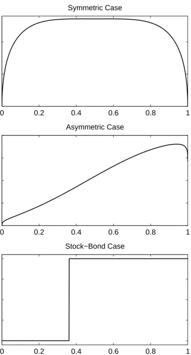
In this section we characterize the model solution by plotting price-dividend ratios, expected returns, return volatility, etc. as a function of the single state variable: the dividend share of the first asset. To illustrate and quantitatively evaluate the model, we present specific numerical examples based on three cases. Throughout these examples, wefix the subjective discount factorδto 0.10, and we set the correlation between the dividend processes to zero. The three cases are:
The Symmetric Case. In this scenario, dividends for the two assets follow identical geometric Brownian motions, µ1 = µ2 = 0.02, andσ1 = σ2 = 0.20. This is the natural simplest case to start with. We can also view this case as a market in which there are two large primary sectors, such asfinancials and industrials.
The Asymmetric Case. In this scenario, dividend volatility for the first asset is higher than for the second asset,µ1 =µ2 = 0.02, σ1= 0.40, andσ2 = 0.20. We can view the first asset as an individual
firm or a small sector and the second asset as the rest of the market. For this interpretation, the region of the state space with a low dividend share is the most interesting. We can also think of the second asset as afirm with unusuallylowcashflow volatility, such as a regulated utility. For this interpretation, high values of thefirst asset’s share (low values of the second asset’s share) are the most interesting. Finally, we can think of thefirst asset as relatively volatile traded securities, and the second asset as relatively safe but less liquid securities such as human capital, real estate, etc.
The Stock-Bond Case. In this scenario, we specify µ1 = 0.03, µ2 = 0.00, σ1 = 0.20, and σ2 = 0.00.
The second tree is a level perpetuity (in positive net supply) with no dividend risk. We allow thefirst tree higher mean dividend growth, as stock dividends typically grow over time while bond (perpetuity) coupons do not. Dividend growth of three percent rather than two percent as in the other cases produces clearer plots. This parameterization allows us to address what is perhaps the most important rebalancing and portfolio issue of all, that of stocks vs. bonds. It also allows us to address “stock” market dynamics that come from market clearing in the overall market for capital, while the returns on the overall wealth portfolio remain i.i.d.
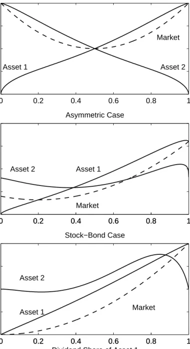
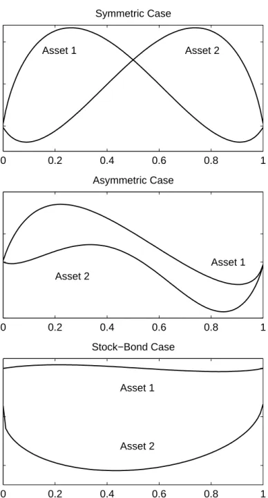
In each plot, the top panel presents the symmetric case; the middle panel, the asymmetric case; and the bottom panel, the stock-bond case.
4.1 Expected Returns and Excess Returns.
Figure 2 plots expected returns and the riskless rate. Figure 3 plots expected excess returns. The often strong dependence of expected returns on the dividend share shown in thesefigures implies that both expected returns and excess returns can display a great deal of time variation even though expected dividend growth rates are constant.
As we expect from Equation (20), the riskless rate in Figure 2 is a quadratic function of the dividend share. The symmetric case in the top panel shows that the riskless rate is higher for intermediate shares,
where dividends are better diversified, consumption volatility is lower, and thus the precautionary savings motive is lower. In the asymmetric case in the middle panel, the quadratic riskless rate is shifted to the left, as thefirst asset is more volatile. There is still some diversification effect, however, as the maximum riskless rate is interior. In the stock-bond case of the bottom panel, consumption growth is also zero and risk free when the risky asset share is zero, so the interest rate equals the discount rate, ten percent. The interest rate rises to an interior maximum, first following the greater mean consumption growth due to the greater mean dividend growth of thefirst asset, but then falling as that assets’ greater volatility induces precautionary saving.
The market expected return in the top two panels of Figure 2 is a constant, as the market price-dividend ratio and mean consumption growth rate are constants. In the bottom panel, the market expected return rises with mean consumption growth as a linear function of the share.
The market expected excessreturn in Figure 3 is then the mirror image of the quadratic riskless rate. Also, the market expected excess return is proportional to consumption volatility in any log utility model, and consumption volatility is lower for intermediate shares.
The expected excess returns for the two individual assets in the symmetric case (Figure 3, top) are monotonic and approximately linear in the dividend share. To understand this behavior, recall that expected excess returns represent risk premia, reflecting the covariance of returns with the discount factor. With log utility,
Et[R1 ] − r dt= Covt R1, dC
C . (37)
Now, return shocks come from dividend growth shocks and shocks to the valuation of dividends,6
R1= dP1 P1 + D1 P1 dt= D1 P1 dt+ dD1 D1 + d(P1/D1) P1/D1 + dD1 D1 d(P1/D1) P1/D1 . (38)
Thus, we can express the covariance of returns with consumption growth as
Et[R1 ] − r dt= Covt dD1 D1 ,dC C + Covt d(P1/D1) P1/D1 ,dC C . (39)
Since consumption growth is the share-weighted sum of dividend growth rates, thefirst term is linear in the dividend share,
Covt dD1 D1 , dC C =sσ 2 1. (40)
6To derive Equation (38), express P1 asD1·(P1/D1) and apply Itˆo’s Lemma. Since dividend growth
is i.i.d., the first two terms on the right hand side of Equation (38) describe the effects on returns of current and expected future changes in cash flows. The remaining terms, and especially the third, capture discount rate effects, the effects on returns of changes in the discount rate applied to future cash
flows. The first two terms also describe returns with no change in the state variable, and the P1/D1
When thefirst asset has a share of zero, the covariance of its dividend growth with that of aggregate consumption — composed entirely of the uncorrelated dividends of the other asset — is zero. As the share increases, the covariance of thefirst asset’s dividends with aggregate consumption increases linearly.
In this way, the approximate linearity of expected excess returns in Figure 3 is natural, and it shows that “cash-flow betas” linear insdominate the covariance of returns with consumption growth in these cases. The deviations from linearity seen in Figure 3 represent the usually smaller effects of “valuation betas,” expected returns corresponding to covariance of the change in the price-dividend ratio with aggregate consumption. These deviations from linearity are perhaps the most interesting part of the model.
In the asymmetric case, the valuation effects are larger. As shown in the middle panel of Figure 3, the expected excess return of thefirst asset is no longer monotonic, as it declines slightly near a share of one. The left-hand scale of the middle panel is larger, reflecting much larger variation in expected excess returns. This comes from the larger variance of dividends and hence consumption growth.
More dramatically, the expected excess return of the second asset declines with its share through much of the range. The expected excess return no longer declines to zero as its share declines to zero, on the right hand side of the lower panel. Here, the entire expected excess return is driven by “valuation risk,” the covariance of the price-dividend ratio with aggregate consumption, even though the “dividend risk,” covariance of dividend growth with aggregate consumption, vanishes.
In the stock-bond case of the lower panel, the expected excess return of the stock shows the usual near-linearity. The long-term bond now also shows a varying expected excess return, despite ariskless
cashflow. This result is driven entirely by discount rate effects of course. The expected excess long-term bond return — the term premium — can be both positive and negative, as found in bond data by Fama and Bliss (1987). As in reality, term premia are much smaller than expected excess stock returns, since there is no premium for cash-flow risk.
The individual-asset expected returns in Figure 2 show a roughly quadratic pattern. We can now most easily understand this pattern as the nearly linear expected excess returns of Figure 3 plus the quadratic riskless rate.
The behavior of expected returns drives many of the results that follow. A positive shock to the
first asset’s dividends has an immediate effect on the asset’s price. However, this shock also changes the dividend share, and hence, affects the asset’s expected return. Where expected excess returns rise in their dividend share, we expect to see positive autocorrelation and momentum of returns. Where expected returns decline in the dividend share, we expect to see negative autocorrelation and mean-reversion. The plots are not monotonic, so both signs are possible. We calculate autocorrelations below, and find this intuition is roughly correct. (It’s not exactly correct since shocks to the second asset’s dividends affect the prices and returns of thefirst asset.)
Changing expected returns take the form of further expected changes in prices, since dividend growth is i.i.d. Thus, dividend shocks may have long-lasting price and return effects. Where expected returns increase in the share, prices will seem initially to “underreact” and “slowly” to incorporate dividend news. Where expected returns decline, prices will seem to “overreact.”
4.2 Price-Dividend Ratios.
Figure 4 plots price-dividend ratios as a function of the dividend share of thefirst asset. From Equation (21), the price-dividend ratio for the market is constant, and equals ten in all three cases. Price-dividend ratios for the individual assets vary widely, however, and need not be monotonic in the share.
Since dividend growth is i.i.d., price-dividend ratios are driven entirely by expected returns. Since the share is highly autocorrelated, today’s expected returns capture a great deal of the future expected returns that drive price-dividend ratios. Hence, the price-dividend ratios in Figure 4 are essentially the inverse of the expected returns of Figure 2, and can be understood as such.
In the upper panel of Figure 4, the limit of the price-dividend ratio for the first asset is 16.67 at zero, and then declines as the share increases. Past a share of 1/2, it becomes even less than the market price-dividend ratio of ten, and then rises slightly tofinish at ten when thefirst asset becomes the entire market. In the asymmetric case of the middle panel, the shapes are the same, but the magnitudes are quite different. Interestingly, the price-dividend ratio for the second asset increases without bound as the share approaches one. The stock-bond case shows variation in the bond price-dividend ratio (the inverse of the coupon yield), despite no cashflow uncertainty.
In each scenario, assets have lower expected returns and higher price-dividend ratios when their share of the total dividends approaches zero than otherwise. Assets are more highly valued when they represent a small share of total dividends, and hence, are more valuable from a diversification perspective. Thus, “small”firms are “growth” firms, in the sense of having high valuations and low expected returns. This phenomenon is particularly strong for a smallfirm with lower dividend volatility, such as the second asset in the asymmetric case in Figure 2, whose expected return is small and whose price-dividend ratio goes to infinity as its share goes to zero.
Our calibrations of the model do not display a separate smallfirm effect. We do not have separate “size” and “value” dimensions to the cross section. In our calibrations, smallfirms generate low average returns and excess returns, whether “small” refers to the dividend share (as seen in Figures 2 and 3), or to market value (not shown). Of course, it is likely in reality that smallfirms have cashflows that are sensitive to aggregate conditions, rather than the uncorrelated cashflows we have specified. This additional ingredient can easily produce high average returns.
The decline of the price-dividend ratio with size is not monotonic however, and we see interior minima in the price-dividend ratio plots. The price-dividend ratio of thefirst asset must be below the price-dividend ratio of the market when the ratio of the second asset is above the ratio of the market, since the share-weighted average price-dividend ratio equals that of the market. As its share approaches one, however, the price-dividend ratio of an asset must converge to the market price-dividend ratio.
The price-dividend ratio of the second asset in the middle panel of Figure 4 gives some insight into the strange behavior of that asset’s expected excess return in Figure 3. In the far right region, where thelow-volatility second asset is a small fraction of the market, its price-dividend ratio is a strongly sloped and nonlinear function of the share. Thus, small changes in the share result in large changes in the assets’ valuation, which is why the valuation covariance term in Equation (39) is so important.
By taking limits of the hypergeometric function, we show in Section 3 of the Appendix that
lim s→0 P1 D1 = 1 δ+ν−η2/2. (41)
This expression holds forθ>1, which implies that the denominator is positive. If θ≤1, the limit is
∞. For the cases withρ= 0 and µ1=µ2, this expression simplifies to
lim s→0 P1 D1 = 1 δ−σ2 2 . (42)
Thus, the price-dividend ratio of the first asset diverges to ∞ if the variance of the second asset is greater than the discount factor, and vice versa. Givenδ= 0.1, the cutoffis σ2 =√0.1 = 0.316. Our asymmetric case withσ1= 0.4 is well above that cutoff, so the second price-dividend ratio does go to
∞as Figure 2 suggests. The price-dividend ratio increases at a rate less than or equal to 1/s, however, since the share-weighted average of the price-dividend ratios must equal the market price-dividend ratio of ten, and the market value must decline to zero ass→0.
To provide some intuition for why the price-dividend ratio can become infinite in this model, recall from Equation (28) that the price-consumption ratio is an exponentially-weighted average of the expected dividend share. SinceD1 =sC, the price-dividend ratio is simply 1/stimes the
price-consumption ratio, and we can write
P1 D1 =Et ∞ 0 e−δτ st+τ st dτ . (43)
Thus, the price-dividend ratio can be expressed as an exponentially-weighted average of expected divi-dend share growth rates. When the dividivi-dend share of an asset is expected to grow at a rate faster than
eδτ, the integral in Equation (43), and hence the price-dividend ratio, can diverge. This feature parallels the result from the classical Gordon growth model in which the price-dividend ratio for a stream of dividends can be infinite if the dividend growth rate exceeds the discount rate. Now, since 0≤s≤1,
scannot growth faster thaneδτ forever, for anyfinite initials. Hence, the price-dividend ratio isfinite for anyfinites. In the limit ass→0, however, we also havest+τ→0, but the latter occurs at a slower rate, so that the share does grow sufficiently fast to give an infinite price-dividend ratio.
4.3 Price-Dividend Ratios and Expected Returns.
Comparing expected returns and excess returns in Figures 2 and 3 with price-dividend ratios in Figure 4, one suspects that price-dividend ratios forecast expected returns and excess returns, since they vary in inverse ways with the dividend share. Following up on this intuition, Figure 5 plots expected returns and excess returns versus the dividend-price ratios. In all three cases, expected returns are not far from a linear function of the dividend-price ratio. The quadratic shape of expected returns and the quadratic shape of price-dividend ratios as functions of the share about offset. Expectedexcessreturns show interesting nonlinearities at high dividend-price ratios, corresponding to low price-dividend ratios at high dividend shares. The price-dividend ratio is not a monotonic function of the share (Figure 4). Hence, even when the expected excess return is a monotonic function of theshare, we will see the interesting nonlinear relations shown in Figure 5.
The asymmetric calibration in the middle panel is useful for thinking about individualfirms vs. the market, and hence in considering cross-sectional relations from the empirical literature. We see here that “value”firms with high dividend-price ratios also have high average returns and excess returns. The stock-bond calibration in the lower panel allows us to compare the model to regressions of stock market returns on dividend yields, following Fama and French (1988). Both calibrations give a reasonable quantitative as well as qualitative fit. In each case, the slope is about one — a one percentage point increase in the dividend-price ratio corresponds to a one percentage point increase in expected return and excess return. This is about the magnitude suggested by both investigations of the cross section of stocks and time series regressions of returns on dividend-price ratios for the stock market as a whole.
For a cross-sectional example, Cohen, Polk, and Vuolteenaho (2003, Table 1, p. 619) report a regression coefficient of log one-year return on log book-market ratio of 0.027, where the regression is taken across book-market sorted portfolios. The coefficient of about one for returns on the dividend-price ratio in Figure 5 corresponds to a coefficient of about 0.04 for log returns on thelogdividend-price
ratio, linearizing around a typical four percent dividend-price ratio. Since price rather than book or dividend is the important right-hand-side variable in these regressions, these coefficients are comparable. The model thus produces if anything a slightly stronger regression than found by Cohen, Polk, and Vuolteenaho.
Fama and French (1992, Table IV, p. 442) sortfirms by book-market and report average returns of the book-market sorted portfolios. A regression of Fama and French’s average monthly percent return on their log book-market ratios across their 13 portfolios gives a coefficient of 0.50, and a plot shows a reasonably linear relation. One can also see this result in the simple spreads: Fama and French’s average returns vary from 0.3 percent to 1.83 percent across portfolios, and log book-market varies from−2.22 to 1.02, giving a slope of about 0.5. Converting to annual net (not percent) returns, Fama and French’s evidence implies a coefficient of about 12 × 0.005 = 0.06, a little higher this time than the 0.04 suggested by Figure 5.
In time-series regressions for overall stock market indices, Fama and French (1988, Table III, p. 12) report coefficients between 2.35 and 5.37 in the full sample. However, the high returns of the 1990s despite ever lower dividend-price ratios has brought down the estimate somewhat. Cochrane (2001, Ch. 20) surveys the evidence and argues for a coefficient of about two. Others express even lower views. As in the empirical literature, the return regression and the excess return plots of Figure 5 produce quite similar coefficients. Variation in price-dividend ratios is driven by variation in risk premia more than by variation in the riskless rate.
The stock-bond calibration contrasts starkly to results we would obtain with the total market, i.e. wealth portfolio or consumption claim. In this model, the total market price-dividend ratio is constant. It cannot forecast the equally constant market expected return, nor the time-varying market expected excess return. However, Fama and French’s (1988) regressions apply to the stock market only. We see in the bottom panel of Figure 5 that the stock portion of the market may be forecastable from its price-dividend ratio, even when the total market is not. In this case, the stock market is subject to market-clearing induced dynamics: as its share gets larger, its expected return rises (Figures 2 and 3) to induce investors to keep holding the larger share. The price-dividend ratio falls, reflecting and forecasting that higher expected return.
In sum, simple market-clearing mechanics generate both short-run continuation and momentum in stocks, and simultaneously long-run mean reversion as evidenced by dividend-yield predictability in both individual stocks and in the stock market as a whole.
4.4 Return Volatility.
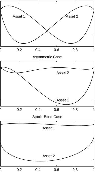
Figure 6 plots the standard deviation of market and individual-asset returns as a function of the div-idend share. In the one-tree model, return volatility is constant and equals divdiv-idend volatility. Here, market return volatility mirrors consumption growth volatility. Market volatility is generally lower for intermediate values of the dividend share where the market diversifies between the two securities.
In the symmetric case (top panel of Figure 6), return volatility starts at the 0.20 volatility of the dividend process when the share is zero, but then varies as an S−shaped function of the dividend share. For dividend shares greater than about 0.8, the volatility of asset returns exceeds the volatility of the underlying cashflows or dividends. This result implies “excess volatility” in the sense that return volatility is higher than the volatility of the fundamental cashflows. There are two forces at work here. First, this is the region in which expected returns in Figure 2 are a declining function of the share, so prices “overreact” to dividends. A positive shock to thefirst asset’s dividends thus raises the price of thefirst asset by more than the dividend shock. Second, shocks to the second asset’s dividends affect the price of thefirst asset even with no news about thefirst asset’s dividends.
For shares below 0.8, return volatility is less than dividend growth volatility. Here, expected returns are a positive function of the share in Figure 2, so prices “underreact” to dividend news. In this region, this effect is large enough to overwhelm volatility in thefirst asset’s returns induced by shocks to the second asset’s dividends.
In the asymmetric case (the middle panel of Figure 6), the first asset’s return volatility follows a similar S−shaped function of the share. The second asset displays about the same volatility as that of the assets in the top panel, though it’s harder to see in the necessarily larger scale of the middle panel. Interestingly, the second asset’s return volatility is less than its dividend volatility even in the limit as its share goes to zero, on the right hand side of the bottom panel. This result again reflects the explosive behavior of its price-dividend ratio in this region. In this region, a small increase in dividends brings a much lower price-dividend ratio, so the return is less than the dividend increase.
The volatility of thefirst asset in the stock-bond case is similar to the above cases. However, there is only a very small and barely visible region of “excess volatility,” where return volatility is larger than dividend growth volatility. This occurs for two reasons. First, there is only a small region in Figure 3 where expected excess returns decline in the share, where a shock to thefirst asset’s dividends causes prices to rise more than dividends. Second, there are no shocks to the second asset’s dividends to move the price of thefirst asset in the absence of news about its dividends.
In the stock-bond case, the second asset shows an interesting volatility pattern with two lobes. The price-dividend ratio in Figure 4 is a non-monotonic function of the share, and there are no shocks to the bond’s dividends. Thus, where the bond’s price-dividend ratio is declining, bond returns are negatively correlated with stock dividends and aggregate consumption growth. Where the bond price-dividend ratio is rising, bond returns are positively correlated with aggregate consumption growth. Where the bond price-dividend ratio is flat, bond returns are riskless, as neither the price nor the dividend can change. For this reason there are two humps and a zero in the plot of the standard deviation of bond returns.
The volatility of the stock is larger than the volatility of the total market, which here equals consumption growth. This is an important feature of the data. If we think of the total market as including bonds, so a typical stock share is 0.6, this effect is not a quantitative match, however, as the model’s consumption growth volatility is still 12 percent. If we think of the total market as including all wealth, such as real estate, human capital, etc., then a reasonable share is 0.2 or less, and the model does begin to capture the fact that stock returns with σ = 18 percent are much more volatile than consumption growth withσ <4 percent. However, this result is fairly mechanical in this calibration of the model, as the price effects are small. Stock return volatility is driven here primarily by the volatility of its dividend stream, where actual aggregate stock market return volatility of about 16 percent is substantially higher than (and less correlated with) its roughly 11 percent dividend growth volatility. Comparing the expected excess returns in Figure 3 with the return volatility in Figure 6, we see that Sharpe ratios vary considerably over time as the dividend share varies.
4.5 Market Betas.
With log utility, expected returns follow a conditional CAPM and consumption CAPM. Figure 7 plots the instantaneous betas. Of course, betas are implied by the expected excess return plots of Figure 3. However, it’s still worthwhile to consider betas directly. The strong variation of betas with share in Figure 7 shows that betas will vary over time for individual stocks and portfolios.
For the symmetric case in the top panel, the beta for thefirst asset is zero when the share is zero. As we have seen, the return covariance is equal to the dividend covariance here, and the first asset’s dividends are uncorrelated with those of the second asset, which is now the entire market. As the share
increases, however, thefirst asset contributes more to the total market return and its beta increases correspondingly. The beta eventually becomes greater than one for values of the share above 50 percent. As the share approaches one, the beta begins to decrease and eventually converges to one. When the share is one, thefirst asset is the entire market and its beta with itself has to equal one. The nearly linear expected excess return plot of Figure 3 is thus composed of this interesting nonlinear beta and the quadratic market expected excess return of Figure 4.
It’s initially puzzling that the beta can be greater than one. However, the share-weighted average beta must be one. Thus, if the beta of the second asset is less than one, the beta of thefirst asset must be greater than one. More generally, a regression ofxonsx+ (1−s)ywithx, yindependent and identically distributed gives a coefficient s
s2+(1−s)2, which exceeds one for s > 1/2, so a beta greater
than one is not unexpected.
The asymmetric case in the middle panel of Figure 7 is similar, but as usual shifted to the left. Thefirst asset’s beta increases more rapidly and reaches a maximum of about 1.50 near a 50 percent share. Interestingly, the beta for the second asset remains well above zero even in the right-hand limit as the second asset’s share approaches zero. This mirrors the behavior found in the previous graphs: the expected excess return approaches a nonzero limit, and the price-dividend ratio explodes. Although the dividend stream becomes riskless and uncorrelated with aggregate consumption, changes in the valuation of that stream are not riskless, and remain correlated with aggregate consumption. There is no contradiction here with the identity that share averaged betas must equal one, as the share of the second asset approaches zero.
The stock-bond case in the bottom panel shows substantially different behavior. As the share approaches one, the stock beta approaches one and the bond beta approaches zero, since the stock becomes the entire wealth portfolio. For lower shares, the stock beta increases dramatically while the bond beta passes through zero and becomes negative. In this calibration, the only shocks are shocks to the stock’s (thefirst asset’s) dividends. Figure 4 shows that the bond price-dividend ratio is a declining function of the share to abouts= 0.35 and a rising function thereafter. Hence, we expect a negative beta for the second asset on thefirst asset’s dividends belows= 0.35 and a positive beta thereafter, as we see in Figure 7. The large magnitude of thefirst asset’s beta also follows. When the share is small, a one percent market return requires a change in thefirst asset’s dividend of about one percent of total market wealth. Such a change is a large proportional change, implying a huge return for thefirst asset. Beta is the change in the asset’s return corresponding to a one percentage point change in the market return, and it will hence be a large number in this region. Interestingly, the beta of the second asset does not have to converge to one as the second asset becomes the whole market, since the whole market becomes riskless in that limit.
4.6 Serial Correlation of Returns.
Figure 8 graphs the conditional serial correlation of one-year asset returns as a function of the initial dividend share, Corrt[Rt,t+1, Rt+1,t+2|st=s], where Rt,t+1 denotes the discrete-time return from
timetto timet+ 1. To calculate this correlation, we simulate 10,000,000 paths using the same random number generator seed for each initial value of the dividend share. We use the initial value of the dividend throughout the year. As before, since the share does not have a well-defined unconditional density, we cannot present the unconditional correlation and other moments, so we present correlations conditional on the current statest.
Asset returns are serially correlated in all cases. In the symmetric case shown in the top panel, the serial correlations are generally positive, indicating positive momentum. The serial correlations are generally largest in the region where expected returns rise with the dividend share, as one would expect. However, nonlinearities in the share process and the fact that thefirst asset’s returns are also driven
by shocks to the second asset’s dividends mean that this is not a perfect correspondence.
In the asymmetric scenario shown in the middle panel of Figure 8, thefirst asset displays a similar pattern. However, the magnitude of the serial correlation for the first asset is about twice as large. Interestingly, the second asset — the “rest of the market” — is now generally negatively serially correlated, showing “mean-reversion” rather than “momentum.” This calibration is consistent with the general
finding that momentum is a feature of individual stocks, not of the market as a whole.
Finally, in the stock-bond case shown in Figure 1, the serial correlation for thefirst asset is slightly positive for almost all values of the dividend share. In contrast, the serial correlation of the second asset is negative and large for all values of the dividend share, reaching a value of about−0.17 when the dividend share is around 0.85. The negative value is what one expects of bonds: when ex-post bond returns are large, prices rise, and yields and subsequent returns fall. Furthermore, since bonds only move on discount rate news and not on cashflow news, the current bond return is a purer signal of a change in subsequent expected returns.
Although not shown, simulations also indicate that there is a horizon-dependent component to the serial correlations of return. For example, the serial correlation of short-horizon returns for an asset can have a different sign than the serial correlation of long-horizon returns for that asset.
Figure 9 graphs the cross-serial correlations for the three scenarios. In the top panel for the symmetric case, the curve labeled asset one designates the correlation between the return over the next year for thefirst asset and return over the subsequent year for the second asset, and vice versa for the curve titled second asset.
As shown, the cross-serial correlations in the symmetric case are generally negative and roughly of the same order of magnitude of the serial correlations. They are similarly related to the expected return plots. A high return to the second asset lowers the share of thefirst asset, lowering the expected return of thefirst asset. The cross-serial correlation from the second asset to thefirst asset is strongest and negative where thefirst asset has the steepest plot of expected return vs. the share.
In the asymmetric case, the cross-serial correlation can attain large negative values. In particular, the cross-serial correlation for the return on the first asset and the subsequent return on the second asset is nearly−0.06 when the dividend share is about 70 percent. This fact implies that returns on the more volatilefirst asset have considerable predictive power for the subsequent returns on the “rest of the market.”
Finally, in the stock-bond scenario, the cross-serial correlations patterns are again similar to those of the serial correlations shown in Figure 8. The bottom panel of Figure 9 shows that returns on the bond have strong predictive ability for the subsequent returns on the stock. Again, bond returns only move on discount rate effects.
The size as well as the signs of the autocorrelations and cross-serial correlations are about what one would expect from the expected return plots in Figure 2. For example, in the symmetric case, the expected return rises about 4 percentage points as the share rises from 0 to 1. Now, a one percent dividend shock is about a one percent return shock, and it changes the share bys(1−s)×1 percentage points. Thus, in the middle, we expect to see a 4×s(1−s)/100 = 0.01 autocorrelation coefficient. Where the slope of expected return as a function of share is lower or negative, we expect to see a corresponding autocorrelation, multiplied by the quadratic terms(1−s). This reasoning well describes the shape and magnitude of the autocorrelation and cross-serial correlation plots.
correlations somewhat larger than these values. Typical estimates are consistent with a forecastR2 of
0.01 and thus autocorrelations on the order of 0.10. For example, Fama and French (1986) report 1.5 percent per month return from a strategy that goes long the past year winners and short the past year losers. The average return of the top decile of a normal distribution is 1.76 standard deviations above the mean. Therefore, using a 50 percent standard deviation of individual stock returns and a ten percent average stock return, the winning decile typically earned 10 + 1.76×50 = 100 percent in the past year, and the losing decile lost 10−1.76×50 = 80 percent. A serial correlation (or regression) coefficient of ten percent then implies that the long-short strategy is expected to earn (100 + 80)×0.1 = 18 percent in the following year, or 1.5 percent per month. Negative cross-serial correlation helps of course; a 0.05 own-serial correlation and 0.05 cross-serial correlation coefficient will have the same effect. Still, these numbers are a factor offive larger than what we see. Again, our model provides a qualitative but not a quantitative match to the data.
The autocorrelations die to zero as the share declines to zero. Even a doubling of value by a small
firm has a small total impact on the share. Since expected returns are roughly linear in the share, this event has a small effect on subsequent expected returns. Thus, market-clearing mechanics can shed insight on momentum in portfolios, such as the industry portfolios in Grinblatt and Moskowitz (1999), but market-clearing mechanics will not deliver much insight into momentum driven by autocorrelation and cross-serial correlation of small individual stock returns.
4.7 Return Correlations.
There can be significant correlationbetween the two asset returns, even when the underlying dividend processes are uncorrelated as in our scenarios. A shock to thefirst asset affects the discount factor for the second asset.
Figure 10 plots the conditional correlation coefficient between the instantaneous returns of the two assets as a function of the dividend share, Corrt[R1,t, R2,t|st=s]. We calculate this correlation
directly from the volatility terms in the instantaneous return formula, Equation (34).
In the symmetric case shown in the top panel, the correlation is equal to zero when the share is near the endpoints. As we have seen above, return variation is dominated by dividend variation here, and the dividends are uncorrelated with each other. For intermediate values of the share, however, the return correlation rises to nearly 14 percent. A “common factor” or “contagion effect” appears in returns, even though there is none in cashflows.
The mechanism for correlation, as usual, traces back to expected returns as a function of the share. When the dividend of the second asset increases, the share of thefirst asset decreases, decreasing the expected return of thefirst asset. Lower expected return means higher prices, and a positive ex-post return on thefirst asset. Shocks to thefirst asset affect the second asset’s returns in the same way, and the correlation represents the sum of the two effects.
The return correlation can be significantly higher, and it is so in the asymmetric case. In this case, the correlation between asset returns is greater than 70 percent for large shares. For a large share of the volatile asset, consumption growth becomes very volatile. This large volatility gives large discount rate effects to the second asset’s price, overwhelming its smaller cash flow effects. Afirm (the second asset) whose cashflows are muchlessvolatile than those of the rest of the market will have returns that are much more influenced by market movements than those of otherfirms.
In the stock-bond case, the first asset’s dividends are the only shock, so returns are perfectly correlated. The sign of the correlation switches from−1 to +1 as the slope of the bond price-dividend ratio as a function of share, and thus the beta, switches sign from negative to positive.
The difference in the pattern of correlation between the cases shows that the cross-sectional struc-ture of the market, in terms of dividend shares and volatilities, can have a large effect on the joint distribution and factor structure of asset returns.
5. THE INVERSE PORTFOLIO CHOICE PROBLEM
One of the most familiar paradigms infinance is the traditional dynamic portfolio-choice problem of Merton (1971, 1973), Cox, Ingersoll, and Ross (1985), and many others. In this paradigm, investors choose optimal portfolios given the exogenously specified dynamics of prices of assets in the investment opportunity set. To provide additional insight into the role of the market-clearing condition in the two-asset model, we illustrate that this condition enables the solution of theinverseportfolio problem, defined as the problem of inferring the dynamics of asset prices given the composition and optimality of a specific portfolio.
To illustrate the inverse problem as clearly as possible, we assume that there is an agent with log utility for whom an optimal portfolio over time consists of holding a constant number of shares each of assets one and two (the market-clearing condition). Without loss of generality, we assume that the investor holds one share each of the two assets. Thus, the vector of optimal portfolio weightswis given by, w= P1 P1+P2 P2 P1+P2 . (44)
From Merton (1971) Equation (104), however, thefirst-order conditions for the optimality of the in-vestor’s portfolio imply,
w=Σ−1(α−r1), (45)
where 1 is the unit vector,αis the vector of expected asset returns, andΣis the covariance matrix of returns for the two assets. Rearranging thesefirst-order conditions gives,
α=r1 +Σw. (46)
Furthermore, from Merton Equation (102), the envelope condition equating the marginal utilities of the investor’s consumption and wealth implies,
1
C =
1
δW, (47)
orC=δW. Because of the “buy-and-hold” condition, however, optimal consumption must also equal the total dividends received by the investor,C=D1+D2, which, in turn, implies,
W =D1+D2
Having now expressed the value of the investor’s as an explicit function of the dividends, we can apply Itˆo’s Lemma directly to Equation (48) to obtain the moments of the investor’s portfolio,
wα=δ+µ1 D1 D1+D2 +µ2 D2 D1+D2 , (49) wΣw=σ21 D1 D1+D2 2 +σ22 D1 D1+D2 2 + 2ρσ1σ2 D1 D1+D2 D2 D1+D2 . (50)
Now rearranging Equation (46), premultiplying byw, and using the fact that the investor’s portfolio weights sum to one gives,
r=wα−wΣw. (51)
Thus, the riskless rate can be expressed as an explicit function of the dividends after substituting in from Equations (49) and (50).
With these results, we now demonstrate how the inverse problem can be solved. We express the prices of thefirst and second assets asP1(D1, D2) andP2(D1, D2) to denote their functional dependence on the dividends explicitly. An application of Itˆo’s Lemma gives,
dP1= µ1D1 ∂P1 ∂D1 +µ2D2 ∂P1 ∂D2 + σ 2 1D21 ∂2P 1 ∂D21 + 2ρσ1σ2D1D2 ∂2P 1 ∂D1∂D2 +σ 2 2D22 ∂2P 1 ∂D22 /2 dt +σ1D1∂P1 ∂D1 dZ1+σ2D2∂P1 ∂D2 dZ2, (52) dP2= µ1D1∂P2 ∂D1 +µ2D2 ∂P2 ∂D2 + σ 2 1D21 ∂2P2 ∂D2 2 + 2ρσ1σ2D1D2 ∂ 2P2 ∂D1∂D2 +σ 2 2D22 ∂2P2 ∂D2 2 /2 dt +σ1D1 ∂P2 ∂D1dZ1+σ2D2 ∂P2 ∂D2dZ2. (53)
Taking the appropriate expectations gives the following expression for α(recalling that the total ex-pected return includes the dividend yield),
α= µ1D1∂∂D1P1 +µ2D2∂∂D2P1 + σ2 1D12∂ 2P1 ∂D2 1 + 2ρσ1σ2D1D2 ∂2P1 ∂D1∂D2 +σ22D22∂ 2P1 ∂D2 2 /2 +D1 /P1 µ1D1∂∂D1P2 +µ2D2∂∂D2P2 + σ21D12∂∂2DP22 2 + 2ρσ1σ2D1D2 ∂2P2 ∂D1∂D2 +σ 2 2D22∂ 2 P2 ∂D2 2 /2 +D2 /P2 (54) Similarly, the elements of the covariance matrixΣof returns for the two assets are,
Σ11= 1 P2 1 σ21D12∂P1 ∂D1 2 + 2ρσ1σ2D1D2 ∂P1 ∂D1 ∂P1 ∂D2 +σ22D22∂P1 ∂D2 2 (55) Σ12=Σ21= 1 P1P2 σ12D21∂P1 ∂D1 ∂P2 ∂D1 +ρσ1σ2D1D2 ∂P1 ∂D1 ∂P2 ∂D2 + ∂P1 ∂D2 ∂P2 ∂D1 +σ22D22∂P1 ∂D2 ∂P2 ∂D2 (56) Σ22= 1 P2 2 σ21D12∂P2 ∂D1 2 + 2ρσ1σ2D1D2 ∂P2 ∂D1 ∂P2 ∂D2 +σ22D22∂P2 ∂D2 2 (57)
Finally, equating the value ofα in Equation (46) with the value ofα in Equation (54) results in the following system of equations,
σ21D12∂ 2P1 ∂D2 1 /2 +ρσ1σ2D1D2 ∂ 2P1 ∂D1∂D2 +σ22D22∂ 2P1 ∂D2 2 /2 +µ1D1∂P1 ∂D1 +µ2D2∂P1 ∂D2 −(r+Σ11w1+Σ12w2)P1+D1= 0, (58) σ21D12∂ 2P2 ∂D2 2 /2 +ρσ1σ2D1D2 ∂2P2 ∂D1∂D2 +σ22D22∂ 2P2 ∂D2 2 /2 +µ1D1 ∂P2 ∂D1 +µ2D2 ∂P2 ∂D2 −(r+Σ21w1+Σ22w2)P2+D2= 0. (59)
However, sincer,Σ, andware given as explicit functions of the dividends, asset prices, and derivatives of the asset prices, Equations (58) and (59) constitute a system of coupled nonlinear elliptic partial differential equations. Given appropriate boundary conditions, these equations can be solved for the values ofP1 andP2as functions of the underlying dividendsD1andD2. The appendix shows that the
functionsP1 andP2 that solve Equations (58) and (59) are identical to the expressions forP1 andP2
given earlier in Section 3. Once the functions P1 and P2 are obtained, αand Σ are given by simply
taking the appropriate derivatives and substituting into Equations (54) through (57), thereby providing a complete solution to the inverse portfolio problem.
To summarize, the key feature that allows for a solution to the inverse problem is that the investor optimally chooses a fully-invested buy-and-hold portfolio through time. This feature implies that the riskless rate and the moments of his portfolio return can be expressed