Introduction to Sparsity in Signal Processing
1Ivan Selesnick November, 2012 NYU-Poly
1
Introduction
These notes describe how sparsity can be used in several signal processing problems. A common theme throughout these notes is the comparison between the least square solution and the sparsity-based solution. In each case, the sparsity-based solution has a clear advantage. It must be empha-sized that this will not be true in general, unless the signal to be processed is either sparse or has a sparse representation with respect to a known transform.
To keep the explanations as clear as possible, the examples given in these notes are restricted to 1-D signals. However, the concepts, problem formulations, and algorithms can all be used in the multidimensional case as well.
For a broader overview of sparsity and compressed sensing, see the June 2010 special issue of theProceedings of the IEEE [5], the March 2006 issue of Signal Processing [16], or the 2011 workshop SPARS11 [25]. Also see the books [14, 28].
1.1 Underdetermined equations
Consider a system of under-determined system of equations
y=Ax (1)
whereAis anM×N matrix,yis a length-M vector, andxis a length-N vector, where N > M. y= y(0) .. . y(M −1) x= x(0) .. . x(N−1)
1For feedback/corrections, email [email protected]. (Last edit: July 16, 2014)
Support from NSF under Grant CCF-1018020 is gratefully acknowledged.
Matlab software to reproduce the examples in these notes is available on the web or from the author. http://eeweb.poly.edu/iselesni/lecture_notes/sparsity_intro/
The system has more unknowns than equations. The matrix A is wider than it is tall. We will assume thatAAHis invertible, therefore the system of equations (1) has infinitely many solutions.
We will use the`2 and`1 norms, which are defined by:
kxk22:= N−1 X n=0 |x(n)|2 (2) kxk1:= N−1 X n=0 |x(n)|. (3)
Often,kxk22, i. e. the sum of squares, is referred to as the ‘energy’ of x. 1.2 Least squares
A common method to solve (1) is to minimize the energy ofx. arg min
x kxk 2
2 (4a)
such thaty=Ax. (4b)
The solution to (4) is given explicitly as:
x=AH(AAH)−1y (5) whereAHis the complex conjugate transpose (Hermitian transpose) ofA. Whenyis noisy, then it is not desired that the equations (1) be solved exactly. In this case, a common method to approximately solve (1) is to minimize the cost function:
arg min
x ky−Axk 2
2+λkxk22. (6)
The solution to (6) is given explicitly by
x= (AHA+λI)−1AHy. (7) Note that each of (5) and (7) calls for the solution to a system of linear equations. In signal processing, the equations may be very large due toy and/or xbeing long signals (or images, or higher dimensional data). For practical algorithms, it is usually necessary to have fast efficient methods to solve these systems of equations. In many cases, the system of equations have special properties or structure that can be exploited for fast solution. For example, sometimes the Fourier transform can be used. Otherwise, iterative methods such as the conjugate gradient algorithm can be used.
1.3 Sparse solutions
Another approach to solve (1) is to minimize the sum of absolute values ofx. Namely, to solve the optimization problem:
arg min
x kxk1 (8a)
such thaty=Ax (8b)
wherekxk1is the`1norm ofx, defined in (3). Problem (8) is known as the
basis pursuit (BP) problem [11]. Unlike the least-square problem (4), the solution to the BP problem (8) can not be written in explicit form. The solution can be found only by running an iterative numerical algorithm.
Whenyis noisy, then it does not make sense to solve (1) exactly, as noted above. In this case, an approximate solution can be found by minimizing the cost function
arg min
x ky−Axk 2
2+λkxk1. (9)
Problem (9) is known as thebasis pursuit denoising (BPD) problem. Like (8), the BPD problem can not be solved in explicit form. It can be solved only using an iterative numerical algorithm. The BPD problem is also referred to as the ‘lasso’ problem (least absolute shrinkage and selection operator) [29]. The lasso problem is equivalent to (9), except that it is defined via a constraint on the `1 norm.
Even though (4) and (8) are quite similar, it turns out that the solutions are quite different. Likewise, even though (6) and (9) are quite similar, the solutions are quite different. In (4) the values|x(n)|2are penalized, while
in (8) the values|x(n)|are penalized. The only difference is the squaring operation. Note that, when a set of values are squared and then summed to get s, the sum s is most sensitive to the largest values, as illustrated in Fig. 1. Therefore, when minimizing kxk22 it is especially important that the largest values ofxbe made small as they count much more than the smallest values. For this reason, solutions obtained by minimizing
kxk22 usually have many small values, as they are relatively unimportant. Consequently, the least square solution is usually notsparse.
Therefore, when it is known or expected that the solutionxis sparse, it is advantageous to use the`1norm instead of the`2norm. Some examples
will be shown in the following sections.
x x2 |x| 1 2 1 2 0 t f(t) (|t|+✏)p a+b|t| t0 x f(x) f(x) =x f(x) = sinx f(x) = 1 20e x Figure 1: The functions|x|andx2.
1.4 Algorithms for sparse solutions
The solution to the basis pursuit problem (8) and basis pursuit denoising problem (9) can not be found using any explicit formula. These problems can be solved only by running iterative numerical algorithms. Note that
kxk1is not differentiable because it is defined as the sum of absolute values.
The absolution value function is not differentiable at zero. The fact that the cost functions (8a) and (9) are non-differentiable makes solving the BP and BPD problems somewhat difficult, especially for large-scale problems. However, the BP and BPD problems are convex optimization problems, and due to this property, there will not be extraneous local minima. In addition, there are many theoretical results and practical algorithms from optimization theory developed specifically for convex optimization prob-lems [9].
Several different algorithms have been developed for solving the BP and BPD problems [8, 12]. There has been some effort by different groups to develop good algorithms for these and related algorithms. A good algo-rithm is one that converges fast to the solution and has low computational cost. The speed of convergence can be measured in terms of the num-ber of iterations or in terms of execution time. An early algorithm to solve the BPD problem is the ‘iterative shrinkage/thresholding algorithm’
(ISTA) [12, 13, 15], which has the property that the cost function is guar-anteed to decrease on each iteration of the algorithm. However, ISTA con-verges slowly for some problems. A more recent algorithm is ‘fast ISTA’ (FISTA) [6]; although the cost function may increase on some iterations, FISTA has much faster convergence than ISTA. FISTA has the unusually good property of having quadratic convergence rate. Another recent al-gorithm is the ‘split variable augmented Lagrangian shrinkage alal-gorithm’ (SALSA) [1, 2]. SALSA often has very good convergence properties in practice. SALSA requires solving a least square problem at each iteration, so it is not always practical. However, in many cases (as in the examples below) the least square problem can be solved very easily, and in these cases SALSA is a very effective algorithm.
For signal processing applications, it is also desired of algorithms for BP and BPD that they do not require the matrix Ato be explicitly stored, but instead require only functions to multiply A and AH with vectors. An algorithm of this kind is sometimes called ‘matrix-free’. For example, if A is a filter convolution matrix, then the matrix-vector product Ax can be computed using fast FFT-based convolution algorithms or using a difference equation. That is faster than performing full matrix-vector multiplication. It also saves memory: it is necessary to store only the impulse response or frequency response of the filter — the actual matrix A itself is never needed. This is especially important in signal processing because the matrixAwould often be extremely large. For a large matrix A, (i) a lot of storage memory is needed and (ii) computing the matrix-vector product Ax is slow. Hence matrix-free algorithms are especially important whenAis large.
Parseval frames
If the matrix Asatisfies the equation
AAH=pI (10)
for some positive number p, then the columns of A are said to form a ‘Parseval frame’ (or ‘tight frame’). This kind of matrix is like a unitary (or orthonormal) matrix, except here A can be rectangular. (A unitary matrix must be square.)
Note that a rectangular matrix can not have an inverse, but it can have either a left or right inverse. If a rectangular matrixAsatisfies (10), then the right inverse of AisAH(Ahas no left inverse).
As a special case of (5), ifAsatisfies the equation (10) then (5) becomes
x=AH(AAH)−1y= 1 pA
Hy
(AAH=pI) (11)
which is computationally more efficient than (5) because no matrix inver-sion is needed.
As a special case of (7), ifAsatisfies the equation (10), then (7) becomes
x= (AHA+λI)−1AHy= 1 λ+pA
Hy (AAH=pI) (12)
which is computationally more efficient than (7) because, again, no matrix inversion is needed. To derive (12) from (7) the ‘matrix inverse lemma’ can be used.
IfAsatisfies (10), then as (11) and (12) show, it is very easy to find least square solutions. It turns out that ifAsatisfies (10), then some algorithms for BP and BPD also become computationally easier.
1.5 Exercises 1. Prove (5).
2. Prove (7).
3. Prove (12). The ‘matrix inverse lemma’ can be used.
2
Sparse Fourier coefficients using BP
The Fourier transform of a signal tells how to write the signal as a sum of sinusoids. In this way, it tells what frequencies are present in a signal. However, the Fourier transform is not the only way to write a signal as a sum of sinusoids, especially for discrete signals of finite length. In the following example, it will be shown that basis pursuit (`1 norm
minimiza-tion) can be used to obtain a frequency spectrum more sparse than that obtained using the Fourier transform.
Suppose that theM-point signal y(m) is written as y(m) = N−1 X n=0 c(n) exp j2π Nmn , 0≤m≤M −1 (13) where c(n) is a length-N coefficient sequence, with M ≤ N. In vector notation, the equation (13) can be expressed as
y=Ac (14)
where Ais a matrix of sizeM×N given by Am,n= exp j2π Nmn , 0≤m≤M −1, 0≤n≤N−1 (15) and c is a length-N vector. The coefficients c(n) are frequency-domain (Fourier) coefficients.
Some remarks regarding the matrixAdefined in (15):
1. If N =M, then Ais the inverse N-point DFT matrix (except for a normalization constant).
2. If N > M, then A is the firstM rows of the inverse N-point DFT matrix (except for a normalization constant). Therefore, multiplying a vector by AorAH can be done very efficiently using the FFT. For example, in Matlab,y=Accan be implemented using the function:
function y = A(c, M, N) v = N * ifft(c); y = v(1:M); end
Similarly, AHy can be obtained by zero-padding and computing the DFT. In Matlab, we can implementc=AHyas the function:
function c = AT(y, M, N)
c = fft([y; zeros(N-M, 1)]); end
Because the matrices A andAH can be multiplied with vectors effi-ciently using the FFT without actually creating or storing the matrix A, matrix-free algorithms can be readily used.
3. Due to the orthogonality properties of complex sinusoids, the matrix Asatisfies:
AAH=NIM (16)
so
(AAH)−1= 1
N IM. (17)
That is, the matrixAdefined in (15) satisfies (10).
WhenN =M, then the coefficientscsatisfying (14) are uniquely deter-mined and can be found using the discrete Fourier transform (DFT). But whenN > M, there are more coefficients than signal values and the coeffi-cientscare not unique. Any vectorcsatisfyingy=Accan be considered a valid set of coefficients. To find a particular solution we can minimize eitherkck22orkck1. That is, we can solve either the least square problem:
arg min
c kck 2
2 (18a)
such thaty=Ac (18b)
or the basis pursuit problem:
arg min
c kck1 (19a)
such thaty=Ac. (19b)
The two solutions can be quite different, as illustrated below.
From Section 1.2, the solution to the least square problem (18) is given by
c=AH(AAH)−1y= 1 NA
Hy (least square solution) (20)
where we have used (17). As noted above, AHy is equivalent to zero-padding the length-M signalyto length-Nand computing its DFT. Hence, the least square solution is simply the DFT of the zero-padded signal. The solution to the basis pursuit problem (19) must be found using an iterative numerical algorithm.
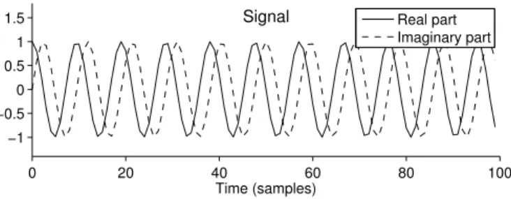
0 20 40 60 80 100 −1 −0.5 0 0.5 1 1.5 Time (samples)
Signal Real part
Imaginary part
Figure 2: The signal is a complex sinusoid.
Example
A simple length-100 signal yis shown in Fig. 2. The signal is given by:
y(m) = exp (j2πfom/M), 0≤m≤M−1, f0= 10.5, M = 100.
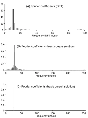
This signal is 10.5 cycles of a complex sinusoid (not a whole number of cy-cles). IfN = 100, then the coefficientscsatisfyingy=Acare unique (and can be found using the DFT) and the unique c is illustrated in Fig. 3a. It can be seen that even though the signal y(m) consists of a single fre-quency, the Fourier coefficients are spread out. This is the famous leakage phenomenon; it occurs whenever a sinusoidal signal has a fractional num-ber of cycles (here, 10.5 cycles).
To obtain a higher resolution frequency spectrum, we can use more Fourier coefficients than signal values; that is, N > M. We will use N = 256, more than twice M and also a power of two (so a fast radix-2 FFT can be used). In this case, because N > M, the coefficients are not unique. The least square solution, easily computed using (20), is shown in Fig. 3b. Note that the least square solution also exhibits the leakage phenomenon.
To obtain the solution to the basis pursuit problem (19), we have used 100 iterations of an iterative algorithm (SALSA). The basis pursuit solu-tion is shown in Fig. 3c. It is clear in the figure that the basis pursuit solution is more sparse than the least square solution. The basis pursuit solution does not have the leakage phenomenon. The cost function history of the SALSA algorithm for this example is illustrated in Fig. 4. It can be seen that the cost function is not strictly decreasing; however, it does
flatten out eventually as it reaches the minimum value. It is informative to look at the cost function history of an iterative algorithm in order to evaluate its convergence behavior.
2.1 Exercises
1. Show that for the matrixAdefined in (15), the matrix-vector products AxandAHycan be computed using the DFT as described.
2. Show that the matrixAdefined in (15) satisfies (16).
3. Reproduce the example (or similar). Also, repeat the example with different frequencies and signal lengths. Comment on your observa-tions.
0 20 40 60 80 100 0 20 40 60 80 Frequency (DFT index)
(A) Fourier coefficients (DFT)
0 50 100 150 200 250 0 0.1 0.2 0.3 0.4
(B) Fourier coefficients (least square solution)
Frequency (index) 0 50 100 150 200 250 0 0.2 0.4 0.6 0.8 1
(C) Fourier coefficients (basis pursuit solution)
Frequency (index)
Figure 3: Fourier coefficients of the signal in Fig. 2, calculated three different ways. 0 20 40 60 80 100 1 1.5 2 2.5
Cost function history
Iteration
Figure 4: Cost function history of algorithm for basis pursuit solution in Fig. 3c.
3
Denoising using BPD
Digital LTI filters are often used for noise reduction (denoising). If the noise and signal occupy separate frequency bands, and if these frequency bands are known, then an appropriate digital LTI filter can be readily designed so as to remove the noise very effectively. But when the noise and signal overlap in the frequency domain, or if the respective frequency bands are unknown, then it is more difficult to do noise filtering using LTI filters. However, if it is known that the signal to be estimated has sparse (or relatively sparse) Fourier coefficients, then sparsity methods can be used as an alternative to LTI filters for noise reduction, as will be illustrated.
A 500 sample noisy speech waveform is illustrated in Fig. 5a. The speech signal was recorded at a sampling rate of 16,000 samples/second, so the duration of the signal is 31 msec. We write the noisy speech signal y(m) as
y(m) =s(m) +w(m), 0≤m≤M−1, M = 500 (21) wheres(m) is the noise-free speech signal andw(m) is the noise sequence. We have used zero-mean Gaussian IID noise to create the noisy speech signal in Fig. 5a. The frequency spectrum of y is illustrated in Fig. 6a. It was obtained by zero-padding the 500-point signal y to length 1024 and computing the DFT. Due to the DFT coefficients being symmetric (because y is real), only the first half of the DFT is shown in Fig. 6. It can be seen that the noise is not isolated to any specific frequency band.
0 100 200 300 400 500 −0.4 −0.2 0 0.2 0.4 0.6 Noisy signal Time (samples) 0 100 200 300 400 500 −0.4 −0.2 0 0.2 0.4 0.6 Denoising using BPD Time (samples)
Figure 5: Speech waveform: 500 samples at a sampling rate of 16,000 sam-ples/second.
Because the noise is IID, it is uniformly spread in frequency.
Let us assume that the noise-free speech signal s(n) has a sparse set of Fourier coefficients. Then, it is useful to write the noisy speech signal as:
y=Ac+w
where A is the M ×N matrix defined in (15). The noisy speech signal is the length-M vector y, the sparse Fourier coefficients is the length-N vectorc, and the noise is the length-M noise vectorw. Becauseyis noisy, it is suitable to findcby solving either the least square problem
arg min
c ky−Ack 2
2+λkck22 (22)
or the basis pursuit denoising (BPD) problem
arg min
c ky−Ack 2
2+λkck1. (23)
Once cis found (either the least square or BPD solution), an estimate of the speech signal is given by ˆs=Ac. The parameter λmust be set to an
0 100 200 300 400 500 0 0.01 0.02 0.03 0.04
(A) Fourier coefficients (FFT) of noisy signal
Frequency (index) 0 100 200 300 400 500 0 0.02 0.04 0.06
(B) Fourier coefficients (BPD solution)
Frequency (index)
Figure 6: Speech waveform Fourier coefficients. (a) FFT of noisy signal. (b) Fourier coefficients obtained by BPD.
appropriate positive real value according to the noise variance. When the noise has a low variance, thenλshould be chosen to be small. When the noise has a high variance, thenλshould be chosen to be large.
Consider first the solution to the least square problem (22). From Sec-tion 1.2 the least square soluSec-tion is given by
c= (AHA+λI)−1AHy= 1 λ+N A
Hy (AAH=NI) (24)
where we have used (12) and (16). Hence, the least square estimate of the speech signal is given by
ˆs=Ac= N
λ+N y (least square solution).
Note that as λ goes to zero (low noise case), then the least square solu-tion approaches the noisy speech signal. This is appropriate: when there is (almost) no noise, the estimated speech signal should be (almost) the observed signal y. Asλincreases (high noise case), then the least square solution approaches to zero — the noise is attenuated, but so is the signal.
But the estimate ˆs= λ+NN yis only a scaled version of the noisy signal! No real filtering has been achieved. We do not illustrate the least square solution in Fig. 5, because it is the same as the noisy signal except for scaling byN/(λ+N).
For the basis pursuit denoising problem (23), we have used N = 1024. Hence, the Fourier coefficient vectorcwill be of length 1024. To solve the BPD problem, we used 50 iterations of the algorithm SALSA. The Fourier coefficient vectorcobtained by solving BPD is illustrated in Fig. 6b. (Only the first 512 values ofcare shown because the sequence is symmetric.) The estimated speech signal ˆs= Acis illustrated in Fig. 5b. It is clear that the noise has been successfully reduced while the shape of the underlying waveform has been maintained. Moreover, the high frequency component at frequency index 336 visible in Fig. 6 is preserved in the BPD solution, whereas a low-pass filter would have removed it.
Unlike the least square solution, the BPD solution performs denoising as desired. But it should be emphasized that the effectiveness of BPD depends on the coefficients of the signal being sparse (or approximately sparse). Otherwise BPD will not be effective.
3.1 Exercises
1. Reproduce the speech denoising example in this section (or a similar example). Vary the parameter λand observe how the BPD solution changes as a function ofλ. Comment on your observations.
4
Deconvolution using BPD
In some applications, the signal of interest x(m) is not only noisy but is also distorted by an LTI system with impulse responseh(m). For example, an out-of-focus image can be modeled as an in-focus image convolved with a blurring function (point-spread function). For convenience, the example below will involve a one-dimensional signal. In this case, the available data y(m) can be written as
y(m) = (h∗x)(m) +w(m) (25) where ‘∗’ denotes convolution (linear convolution) and w(m) is additive noise. Given the observed data y, we aim to estimate the signal x. We will assume that the sequencehis known.
If xis of lengthN andhis of length L, then y will be of length M = N+L−1. In vector notation, (25) can be written as
y=Hx+w (26)
where y and w are length-M vectors and x is a length-N vector. The matrixHis a convolution (Toeplitz) matrix with the form
H= h0 h1 h0 h2 h1 h0 h2 h1 h0 h2 h1 h2 . (27)
The matrix His of sizeM ×N with M > N (becauseM =N+L−1). Because of the additive noisew, it is suitable to findxby solving either the least square problem:
arg min
x ky−Hxk 2
2+λkxk22 (28)
or the basis pursuit denoising problem:
arg min
x ky−Hxk 2
2+λkxk1. (29)
Consider first the solution to the least square problem (28). From (7) the least square solution is given by
x= (HHH+λI)−1HHy. (30)
When H is a large matrix, we generally wish to avoid computing the solution (30) directly. In fact, we wish to avoid storing H in memory at all. However, note that the convolution matrix Hin (27) is banded with L non-zero diagonals. That is,H is a ‘sparse banded’ matrix. For such matrices, a sparse system solver can be used; i.e., an algorithm specifically designed to solve large systems of equations where the system matrix is a sparse matrix. Therefore, when h is a short sequence, the least square solution (30) can be found efficiently using a solver for sparse banded linear
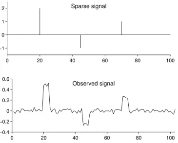
0 20 40 60 80 100 −1 0 1 2 Sparse signal 0 20 40 60 80 100 −0.4 −0.2 0 0.2 0.4 0.6 Observed signal
Figure 7: (a) Sparse signal and (b) observed signaly.
equations. In addition, when using such a solver, it is not necessary to store the matrix Hin its entirety, only the non-zero diagonals.
To compute the solution to the basis pursuit denoising problem (29), we can use the iterative algorithm SALSA. This algorithm can also take advantage of solvers for sparse banded systems, so as to avoid the excessive computational cost and execution time of solving general large system of equations.
Example
A sparse signal is illustrated in Fig. 7a. This signal is convolved by the 4-point moving average filter
h(n) = 1 4 n= 0,1,2,3 0 otherwise
and noise is added to obtain the observed datayillustrated in Fig. 7b. The least square and BPD solutions are illustrated in Fig. 8. In each case, the solution depends heavily on the parameter λ. In these two ex-amples, we have chosenλmanually so as to get as good a solution visually
0 20 40 60 80 100 −0.4 −0.2 0 0.2 0.4 0.6
Deconvolution (least square solution)
0 20 40 60 80 100
−1 0 1
2 Deconvolution (BPD solution)
Figure 8: Deconvolution of observed signal in Fig. 7b. (a) Least square solution. (b) Basis pursuit denoising solution.
as we can. It is clear that the BPD solution is more accurate.
It is important to note that, if the original signal is not sparse, then the BPD method will not work. Its success depends on the original signal being sparse!
4.1 Exercises
1. Reproduce the example (or similar). Show the least square and BPD solutions for different values ofλto illustrate how the solutions depend onλ. Comment on your observations.
5
Missing data estimation using BP
Due to data transmission errors or acquisition errors, some samples of a signal may be lost. In order to conceal these errors, the missing samples must be filled in with suitable values. Filling in missing values in order to conceal errors is callederror concealment [30]. In some applications, part of a signal or image is intentionally deleted, for example in image editing so as to alter the image, or removing corrupted samples of an audio signal.
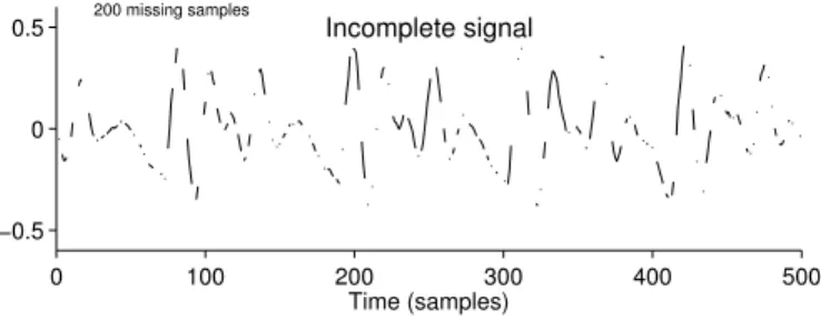
0 100 200 300 400 500 −0.5 0 0.5 Incomplete signal Time (samples) 200 missing samples
Figure 9: Signal with missing samples.
The samples or pixels should be convincingly filled in according to the sur-rounding area. In this case, the problem of filling in missing samples/pixels is often calledinpainting [7]. Error concealment and inpainting both refer to filling in missing samples/pixels of a signal/image.
Several methods have been developed for filling in missing data, for example [17,18,20,21]. In this section, we will describe a method based on sparse signal representations. The example below involves one-dimensional signals, but the method can also be used for images, video, and other multidimensional data.
Fig. 9 shows an example of signal with missing samples. The signal is a speech waveform 500 samples long, but 200 samples are missing. That is, 300 of the 500 samples are known. The problem is to fill in the missing 200 samples.
5.1 Problem statement
Let x be a signal of length M. But suppose only K samples of x are observed, whereK < M. TheK-point incomplete signalycan be written as
y=Sx (31)
whereSis a ‘selection’ (or ‘sampling’) matrix of sizeK×M. For example, if only the first, second and last elements of a 5-point signalxare observed, then the matrix Sis given by:
S= 1 0 0 0 0 0 1 0 0 0 0 0 0 0 1 . (32)
The vectoryis of lengthK(yis shorter vector thanx). It consists of the known samples of x.
The problem can be stated as: Given the incomplete signal y and the matrix S, find x such thaty =Sx. Of course, there are infinitely many solutions. Below, the least square and basis pursuit solutions will be illus-trated. As will be shown, these two solutions are very different.
Properties of S: The matrix Shas the following properties which will be used below.
1. Note that
SST=I (33)
whereIis an K×K identity matrix. For example, forSin (32) have SST= 1 0 0 0 1 0 0 0 1 . 2. Also STS= diag(s) (34)
where the notation diag(s) denotes the diagonal matrix with salong the diagonal. For example, withSin (32) we have
STS= 1 0 0 0 0 0 1 0 0 0 0 0 0 0 0 0 0 0 0 0 0 0 0 0 1
which we can write as
STS= diag([1, 1, 0, 0, 1]).
3. Note that STy has the effect of setting the missing samples to zero. For example, withSin (32) we have
STy= 1 0 0 0 1 0 0 0 0 0 0 0 0 0 1 y(0) y(1) y(2) = y(0) y(1) 0 0 y(2) . (35)
Sparsity Model: Suppose the signal xhas a sparse representation with respect to A, meaning thatxcan be represented as
x=Ac (36)
where cis a sparse coefficient vector of length N withM ≤N, andA is a matrix of size M×N.
The incomplete signalycan then be written as
y=Sx from (31) (37a)
=SAc from (36). (37b)
Therefore, if we can find a vector csatisfying
y=SAc (38)
then we can create an estimate ˆx ofxby setting ˆ
x=Ac. (39)
From (38) it is clear that Sxˆ = y. That is, ˆx agrees with the known samples ofx. The signal ˆxis the same length asx.
Note thatyis shorter than the coefficient vectorc, so there are infinitely many solutions to (38). (yis of lengthK, andcis of lengthN.) Any vector csatisfyingy=SAccan be considered a valid set of coefficients. To find a particular solution we can minimize eitherkck22orkck1. That is, we can
solve either the least square problem:
arg min
c kck 2
2 (40a)
such thaty=SAc (40b)
or the basis pursuit problem:
arg min
c kck1 (41a)
such thaty=SAc. (41b)
The two solutions are very different, as illustrated below. Let us assume thatAsatisfies (10),
AAH=pI, (42)
for some positive real number p.
Consider first the solution to the least square problem. From Section 1.2, the solution to least square problem (40) is given by
c= (SA)H((SA)(SA)H)−1y (43) =AHST(SAAHST)−1y (44) =AHST(pSST)−1y using (10) (45) =AHST(pI)−1y using (33) (46) = 1 pA HSTy (47)
Hence, the least square estimate ˆxis given by
ˆ x=Ac (48) =1 pAA HSTy using (47) (49) =STy using (10). (50)
But the estimate ˆx=STyconsists of setting all the missing values to zero! See (35). No real estimation of the missing values has been achieved. The least square solution is of no use here.
Unlike the least square problem, the solution to the basis pursuit prob-lem (41) can not be found in explicit form. It can be found only by running an iterative numerical algorithm. However, as illustrated in the following example, the BP solution can convincingly fill in the missing samples. Example
Consider the problem of filling in the 200 missing samples of the length 500 signal x illustrated in Fig. 9. The number of known samples isK = 300, the length of the signal to be estimated is M = 500. Short segments of speech can be sparsely represented using the DFT; therefore we set A equal to theM×N matrix defined in (15) where we useN = 1024. Hence the coefficient vector cis of length 1024. To solve the BP problem (41), we have used 100 iterations of a SALSA algorithm.
The coefficient vectorcobtained by solving (41) is illustrated in Fig. 10. (Only the first 512 coefficients are shown because c is symmetric.) The
0 100 200 300 400 500 0 0.02 0.04 0.06 0.08 Estimated coefficients Frequency (DFT index) 0 100 200 300 400 500 −0.5 0 0.5 Estimated signal Time (samples)
Figure 10: Estimation of missing signal values using basis pursuit.
estimated signal ˆx = Ac is also illustrated. The missing samples have been filled in quite accurately.
Unlike the least square solution, the BP solution fills in missing samples in a suitable way. But it should be emphasized that the effectiveness of the BP approach depends on the coefficients of the signal beingsparse(or approximately sparse). For short speech segments, the Fourier transform can be used for sparse representation. Other types of signals may require other transforms.
5.2 Exercises
1. Reproduce the example (or similar). Show the least square and BP solutions for different numbers of missing samples. Comment on your observations.
6
Signal component separation using BP
When a signal contains components with distinct properties, it is some-times useful to separate the signal into its components. If the components occupy distinct frequency bands, then the components can be separated
using conventional LTI filters. However, if the components are not sepa-rated in frequency (or any other transform variable), then the separation of the components is more challenging. For example, a measured signal may contain both (i) transients of unspecified shape and (ii) sustained os-cillations [24]; in order to perform frequency analysis, it can be beneficial to first remove the transients. But if the transient and oscillatory signal components overlap in frequency, then they can not be reliably separated using linear filters. It turns out that sparse representations can be used in this and other signal separation problems [3, 26, 27].
The use of sparsity to separate components of a signal has been called ’morphological component analysis’ (MCA) [26, 27], the idea being that the components have different shape (morphology).
Problem statement
It is desired that the observed signal y be written as the sum of two components, namely,
y=y1+y2 (51)
wherey1andy2are to be determined. Of course, there are infinitely many
ways to solve this problem. For example, one may sety1=yandy2=0.
Or one may sety1arbitrarily and sety2=y−y1. However, it is assumed
that each of the two components have particular properties and that they are distinct from one another. The MCA approach assumes that each of the two components is best described using distinct transforms A1 and
A2, and aims to find the respective coefficientsc1 andc2 such that
y1=A1c1, y2=A2c2. (52)
Therefore, instead of finding y1 andy2 such that y=y1+y2, the MCA
method finds c1 andc2such that
y=A1c1+A2c2. (53)
Of course, there are infinitely many solutions to this problem as well. To find a particular solution, we can use either least squares or basis pursuit. The least squares problem is:
arg min
c1,c2
λ1kc1k22+λ2kc2k22 (54a)
The ‘dual basis pursuit’ problem is:
arg min
c1,c2
λ1kc1k1+λ2kc2k1 (55a)
such thaty=A1c1+A2c2. (55b)
We call (55) ’dual’ BP because of there being two sets of coefficients to be found. However, this problem is equivalent to basis pursuit.
Oncec1andc2 are obtained (using either least squares or dual BP), we
set:
y1=A1c1, y2=A2c2. (56)
Consider first the solution to the least square problem. The solution to the least square problem (54) is given by
µ= 1 λ1 A1AH1+ 1 λ2 A2AH2 −1 y (57a) c1= 1 λ1 AH1µ (57b) c2= 1 λ2 AH2µ. (57c)
If the columns ofA1 andA2 both form Parseval frames, i.e.
A1AH1 =p1I, A2AH2 =p2I, (58)
then the least square solution (57) is given explicitly by
µ= p 1 λ1 + p2 λ2 −1 y (59a) c1= 1 λ1 p 1 λ1 + p2 λ2 −1 AH1y (59b) c2= 1 λ2 p 1 λ1 + p2 λ2 −1 AH2y (59c)
and from (56) the calculated components are
y1= p1 λ1 p1 λ1 + p2 λ2 −1 y (60a) y2= p2 λ2 p 1 λ1 + p2 λ2 −1 y. (60b) 0 50 100 150 −2 0 2 Signal
Figure 11: Signal composed of two distinct components.
But these are onlyscaled versions of the datay. No real signal separation is achieved. The least square solution is of no use here.
Now consider the solution to the dual basis problem (55). It can not be found in explicit form; however, it can be obtained via a numerical algorithm. As illustrated in the following examples, the BP solution can separate a signal into distinct components, unlike the least square solution. This is true, provided that y1 has a sparse representation using A1, and
that y2 has a sparse representation usingA2.
Example 1
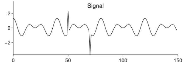
This first example is very simple; however, it clearly illustrates the method. Consider the 150-point signal in Fig. 11. It consists of a few impulses (spikes) and a few sinusoids added together. The goal is to separate the signal into two component signals: one component containing only im-pulses, the other component containing only sinusoids; such that, the sum of the two components equals the original signal.
To use the dual BP problem (55), we need to specify the two transforms A1 and A2. We set A1 to be the identity matrix. We setA2 to be the
overcomplete DFT (15) with size 150×256. Hence the coefficient vector c1 is of length 150, and c2 is of length 256. The coefficients c1 and c2
obtained by solving the dual BP problem (55) are shown in Fig. 12. It can be seen that the coefficients are indeed sparse. (The coefficients c2
are complex valued, so the figure shows the modulus of these coefficients.) Using the coefficients c1 and c2, the components y1 andy2 are obtained
by (56). The resulting components are illustrated in Fig. 12. It is clear that the dual BP method successfully separates the signal into two district
0 50 100 150 −4 −2 0 2 4 Coefficients c1 0 50 100 150 200 250 0 1 2 3 4 5 Coefficients c2 0 50 100 150 −4 −2 0 2 4 Component 1 0 50 100 150 −2 −1 0 1 2 Component 2
Figure 12: Signal separation using dual BP (Example 1). The two components add to give the signal illustrated in Fig. 11.
components: y1contains the impulses, and y2contains the sinusoids.
In this illustrative example, the signal is especially simple, and the sep-aration could probably have been accomplished with a simpler method. The impulses are quite easily identified. However, in the next example, neither component can be so easily identified.
Example 2
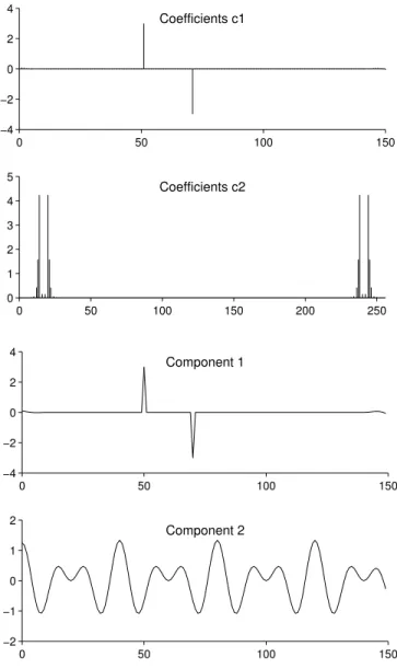
An important property of a voiced speech waveform are the formants (prominent sustained frequencies). Formants are determined by the po-sition of the tongue and lips, etc. (the vocal tract); and can be used to distinguish one vowel from another. Another important property of voiced speech is the pitch frequency, which is determined by the rate at which the vocal chords vibrate. The spectrum of a voiced speech waveform often con-tains many harmonic peaks at multiples of the pitch frequency. The pitch frequency and formants carry distinct information in the speech waveform; and in speech processing, they are estimated using different algorithms.
A speech signal and its spectrogram is shown in Fig. 13. The speech is sampled at 16K samples/second. Both formants and harmonics of the pitch frequency are clearly visible in the spectrogram: harmonics as fine horizontally oriented ridges, formants as broader darker bands.
Roughly, the formants and pitch harmonics can be separated to some degree using dual basis pursuit, provided appropriate transformsA1 and
A2 are employed. We set each of the two transforms to be a short-time
Fourier transform (STFT), but implemented with windows of differing lengths. For A1 we use a short window 32 samples (2 ms) and for A2
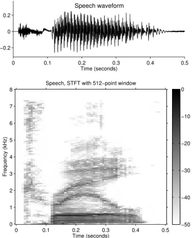
we use a longer window of 512 samples (32 ms). The result of dual BP is illustrated in Fig. 14. The arithmetic sum of the two components is equal to the original speech waveform, as constrained in the dual BP problem formulation. As the figure illustrates, the component y1 consists of brief
complex pulses, each shorter than the pitch period; the component y2
consists of sustained oscillations that are of longer duration. The sustained oscillations visible in y2 constitute the resonant frequencies of the vocal
tract (formants). From the spectrogram of y2, illustrated in Fig. 15, it
can be noted that the pitch harmonics have been substantially attenuated. This further illustrates that, to some degree, the pitch harmonics and
0 0.1 0.2 0.3 0.4 0.5 −0.2 0 0.2 Speech waveform Time (seconds) Frequency (kHz) Time (seconds)
Speech, STFT with 512−point window
0 0.1 0.2 0.3 0.4 0.5 0 1 2 3 4 5 6 7 8 −50 −40 −30 −20 −10 0
Figure 13: A speech waveform and its spectrogram.
formants have been separated into the componentsy1 andy2.
Note that the separation of formants and pitch harmonics is achieved even though the two components overlap in time and frequency. The dual BP procedure, with STFT of short and long windows, achieves this separation through sparse representation.
6.1 Exercises 1. Prove (57).
2. WhenA1 andA2satisfy (10), prove (59a) and (60a).
3. Reproduce the examples (or similar). Show the dual BP solution for
0 0.1 0.2 0.3 0.4 0.5 Speech Component 1 Component 2 Time (seconds) Waveforms (0.5 s) 0.2 0.21 0.22 0.23 0.24 Time (seconds) Waveforms (40 ms)
Figure 14: Speech signal decomposition using dual BP and STFT with short and long windows. The two components add to give the specch waveform illustrated in Fig. 13.
Frequency (kHz)
Time (seconds)
Component 2, STFT with 512−point window
0 0.1 0.2 0.3 0.4 0.5 0 1 2 3 4 5 6 7 8 −50 −40 −30 −20 −10 0
Figure 15: Spectrogram of component 2 in Fig. 14. Compared with Fig. 13 the pitch harmonics are reduced in intensity, but the formants are well preserved.
different parameters λ1 andλ2. Comment on your observations.
7
Conclusion
These notes describe the formulation of several problems. In each case, the least square solution is compared with the solution obtained using `1
norm minimization (either BP or BPD).
1. Signal representation using basis pursuit (BP) is illustrated in Section 2. In the example, a sparse set of Fourier coefficients are obtained which do not exhibit the leakage phenomenon of the least square so-lution. For other types of data, it can be more suitable to use an-other transform, such as the short-time Fourier transform (STFT) or wavelet transforms [10], etc.
2. Signal denoising using basis pursuit denoising (BPD) is illustrated in Section 3. In the example, BPD is used to obtain a sparse set of Fourier coefficients that approximates the noisy signal. Denoising is
achieved because the noise-free signal of interest has a sparse repre-sentation with respect to the Fourier transform. For other types of the data, it can be more appropriate to use other transforms. A transform should be chosen that admits a sparse representation of the underly-ing signal of interest. It was also shown that the least square solution achieves no denoising, only a constant scaling of the noisy data.
3. Deconvolution using BPD is illustrated in Section 4. When the signal to be recovered is sparse, then the use of BPD can provide a more accurate solution than least squares. This approach can also be used when the signal to be recovered is itself not sparse, but admits a sparse representation with respect to a known transform.
4. Missing data estimation using BP is illustrated in Section 5. When the signal to be recovered in its entirety admits a sparse representation with respect to a known transform, then BP exploits this sparsity so as to fill in the missing data. If the data not only has missing samples but is also noisy, then BPD should be used in place of BP. It was shown that the least square solution consists of merely filling in the missing data with zeros.
5. Signal component separation using BP is illustrated in Section 6. When each of the signal components admits a sparse representation with respect to known transforms, and when the transforms are suf-ficiently distinct, then the signal components can be isolated using sparse representations. If the data is not only a mixture of two com-ponents but is also noisy, then BPD should be used in place of BP. It was shown that the least square solution achieves no separation; only a constant scaling of the observed mixed signal.
In each of these examples, the use of the`2 norm in the problem
formu-lation led to solutions that were unsatisfactory. Using the`1norm instead
of the`2norm as in BP and BPD, lead to successful solutions. It should be
emphasized that this is possible because (and only when) the signal to be recovered is either sparse itself or admits a sparse representation with re-spect to a known transform. Hence one problem in using sparsity in signal processing is to identity (or create) suitable transforms for different type
of signals. Numerous specialized transforms have developed, especially for multidimensional signals [19].
In addition to the signal processing problems described in these notes, sparsity-based methods are central to compressed sensing [4].
These notes have intentionally avoided describing how to solve the BP and BPD problems, which can only be solved using iterative numerical algorithms. Algorithms for solving these problems are described in [22,23].
References
[1] M. V. Afonso, J. M. Bioucas-Dias, and M. A. T. Figueiredo. Fast image recovery using variable splitting and constrained optimization.IEEE Trans. Image Process., 19(9):2345–2356, September 2010.
[2] M. V. Afonso, J. M. Bioucas-Dias, and M. A. T. Figueiredo. An augmented Lagrangian approach to the constrained optimization formulation of imag-ing inverse problems. IEEE Trans. Image Process., 20(3):681–695, March 2011.
[3] J.-F. Aujol, G. Aubert, L. Blanc-F´eraud, and A. Chambolle. Image decom-position into a bounded variation component and an oscillating component. J. Math. Imag. Vis., 22:71–88, 2005.
[4] R. G. Baraniuk. Compressive sensing [lecture notes]. IEEE Signal Process-ing Magazine, 24(4):118–121, July 2007.
[5] R. G. Baraniuk, E. Candes, M. Elad, and Y. Ma, editors. Special issue on applications of sparse representation and compressive sensing. Proc. IEEE, 98(6), June 2010.
[6] A. Beck and M. Teboulle. A fast iterative shrinkage-thresholding algorithm for linear inverse problems. SIAM J. Imag. Sci., 2(1):183–202, 2009. [7] M. Bertalmio, L. Vese, G. Sapiro, and S. Osher. Simultaneous structure and
texture image inpainting.IEEE Trans. on Image Processing, 12(8):882–889, August 2003.
[8] S. Boyd, N. Parikh, E. Chu, B. Peleato, and J. Eckstein. Distributed op-timization and statistical learning via the alternating direction method of multipliers.Foundations and Trends in Machine Learning, 3(1):1–122, 2011. [9] S. Boyd and L. Vandenberghe.Convex Optimization. Cambridge University
Press, 2004.
[10] C. S. Burrus, R. A. Gopinath, and H. Guo. Introduction to Wavelets and Wavelet Transforms. Prentice Hall, 1997.
[11] S. Chen, D. L. Donoho, and M. A. Saunders. Atomic decomposition by basis pursuit. SIAM J. Sci. Comput., 20(1):33–61, 1998.
[12] P. L. Combettes and J.-C. Pesquet. Proximal splitting methods in signal processing. In H. H. Bauschke, R. Burachik, P. L. Combettes, V. Elser, D. R. Luke, and H. Wolkowicz, editors,Fixed-Point Algorithms for Inverse Problems in Science and Engineering. Springer-Verlag (New York), 2011.
[13] I. Daubechies, M. Defriese, and C. De Mol. An iterative thresholding algo-rithm for linear inverse problems with a sparsity constraint.Commun. Pure Appl. Math, LVII:1413–1457, 2004.
[14] M. Elad. Sparse and Redundant Representations: From Theory to Applica-tions in Signal and Image Processing. Springer, 2010.
[15] M. Figueiredo and R. Nowak. An EM algorithm for wavelet-based image restoration. IEEE Trans. Image Process., 12(8):906–916, August 2003. [16] R. Gribonval and M. Nielsen, editors. Special issue on sparse approximations
in signal and image processing. Signal Processing, 86(3):415–638, March 2006.
[17] O. G. Guleryuz. Nonlinear approximation based image recovery using adap-tive sparse reconstructions and iterated denoising — Part I: Theory. IEEE Trans. on Image Processing, 15(3):539–554, March 2006.
[18] O. G. Guleryuz. Nonlinear approximation based image recovery using adap-tive sparse reconstructions and iterated denoising — Part II: Adapadap-tive al-gorithms. IEEE Trans. on Image Processing, 15(3):555–571, March 2006. [19] L. Jacques, L. Duval, C. Chaux, and G. Peyr´e. A panorama on multiscale
geometric representations, intertwining spatial, directional and frequency selectivity. Signal Processing, 91(12):2699–2730, December 2011.
[20] A. Kaup, K. Meisinger, and T. Aach. Frequency selective signal extrapola-tion with applicaextrapola-tions to error concealment in image communicaextrapola-tion. Int. J. of Electronics and Communications, 59:147–156, 2005.
[21] K. Meisinger and A. Kaup. Spatiotemporal selective extrapolation for 3-D signals and its applications in video communications. IEEE Trans. on Image Processing, 16(9):2348–2360, September 2007.
[22] I. Selesnick. Sparse signal restoration. Connexions, 2009. http://cnx.org/content/m32168.
[23] I. Selesnick. L1-norm penalized least squares with SALSA. Connexions, 2014. http://cnx.org/content/m48933.
[24] I. W. Selesnick. Resonance-based signal decomposition: A new sparsity-enabled signal analysis method.Signal Processing, 91(12):2793 – 2809, 2011.
[25] Workshop: Signal Processing with Adaptive Sparse
Struc-tured Representations (SPARS11), Edinburgh, June 2011.
http://ecos.maths.ed.ac.uk/SPARS11/.
[26] J.-L. Starck, M. Elad, and D. Donoho. Redundant multiscale transforms and their application for morphological component analysis. Advances in Imaging and Electron Physics, 132:287–348, 2004.
[27] J.-L. Starck, M. Elad, and D. Donoho. Image decomposition via the com-bination of sparse representation and a variational approach. IEEE Trans. Image Process., 14(10):1570–1582, October 2005.
[28] J.-L. Starck, F. Murtagh, and J. M. Fadili. Sparse image and signal pro-cessing: wavelets, curvelets, morphological diversity. Cambridge University Press, 2010.
[29] R. Tibshirani. Regression shrinkage and selection via the lasso. J. Roy. Statist. Soc., Ser. B, 58(1):267–288, 1996.
[30] Y. Wang and Q. Zhu. Error control and concealment for video communica-tion: A review. Proc. IEEE, 86(5):974–997, May 1998.