NBER WORKING PAPER SERIES
DYNAMIC DEBT RUNS Zhiguo He
Wei Xiong Working Paper 15482
http://www.nber.org/papers/w15482
NATIONAL BUREAU OF ECONOMIC RESEARCH 1050 Massachusetts Avenue
Cambridge, MA 02138 November 2009
We thank Viral Acharya, Markus Brunnermeier, Doug Diamond, Itay Goldstein, Milton Harris, Arvind Krishnamurthy, Pete Kyle, Guido Lorenzoni, Stephen Morris, Jonathan Parker, Darius Palia, Adriano Rampini, Michael Roberts, David Romer, Hyun Song Shin, Andrei Shleifer, Amir Sufi, and seminar participants at Chicago, Columbia, Cornell, DePaul, 2009 FESAMES, Federal Reserve Board, Harvard/ MIT, HKMA/BIS, IMF, Kellogg, 2009 Mitsui Finance Symposium at Michigan, 2009 NBER Summer Institute workshops in Monetary Economics and in Capital Markets and the Economy, New York Fed, Philadelphia Fed, Maryland, Minnesota, Notre Dame, Princeton, Texas-Austin, and Wharton for helpful discussion and comments. The views expressed herein are those of the author(s) and do not necessarily reflect the views of the National Bureau of Economic Research.
NBER working papers are circulated for discussion and comment purposes. They have not been peer-reviewed or been subject to the review by the NBER Board of Directors that accompanies official NBER publications.
© 2009 by Zhiguo He and Wei Xiong. All rights reserved. Short sections of text, not to exceed two paragraphs, may be quoted without explicit permission provided that full credit, including © notice, is given to the source.
Dynamic Debt Runs Zhiguo He and Wei Xiong NBER Working Paper No. 15482 November 2009
JEL No. G01,G20
ABSTRACT
We develop a dynamic model of debt runs on a firm, which invests in an illiquid asset by rolling over staggered short-term debt contracts. We derive a unique threshold equilibrium, in which creditors coordinate their asynchronous rollover decisions based on the firm's publicly observable and time-varying fundamental. Fear of the firm's future rollover risk motivates each maturing creditor to run ahead of others even when the firm is still solvent. Our model provides implications on the roles played by volatility, illiquidity and debt maturity in driving debt runs, as well as on firms' capital adequacy standards and credit risk.
Zhiguo He
University of Chicago Booth School of Business [email protected] Wei Xiong
Princeton University Department of Economics Bendheim Center for Finance Princeton, NJ 08450
and NBER
1
Introduction
There is a long history of panic runs on banks. The panic of 1907 led to the creation of the Federal Reserve and the wave of bank failures during the Great Depression led to the establishment of deposit insurance. With the creation of these safeguards, runs on banks have become uncommon in the modern time. However, the structure of the …nancial system has changed in the 21st century, with rapid growth of the share of assets held by non-bank …nancial institutions such as investment banks, special investment vehicles, conduits, and hedge funds. According to U.S. Treasury Secretary Timothy Geithner (2008), the size of the non-bank …nancial system had already surpassed that of the traditional banking system by early 2007. Non-bank institutions do not accept deposits like banks; instead, they rely on short-term debt contracts such as commercial paper and repo transactions to …nance their long-term risky and relatively illiquid assets. Without the protection of deposit insurance, the non-bank …nancial institutions are intrinsically vulnerable to panic runs. In fact, many regulators and researchers, e.g., Bernanke (2008), Cox (2008), Geithner (2008), Brunnermeier (2009), Gorton (2008), Krishnamurthy (2009), and Shin (2009), describe runs on the non-bank …nancial institutions as one of the main causes of the credit crisis of 2007-2008.1
This crisis raises many important policy and academic questions, which require a the-oretical framework to analyze panic runs on …nancial institutions. Diamond and Dybvig (1983) provide a classic bank-run model to show that failure of depositors to coordinate their withdrawal decisions could lead to a self-ful…lling bank-run equilibrium. In this equi-librium, all depositors choose to withdraw from a solvent but illiquid bank, thus causing it to fail prematurely.
Two particular features of …nancial institutions motivate new perspectives on the coor-dination problem between their creditors. First, the assets held by …nancial institutions are mostly …nancial securities whose fundamentals change over time. The fact that runs on the …nancial institutions started in 2007 after their losses from mortgage related holdings became publicly known, e.g., Gorton (2008), suggests that ‡uctuating fundamentals played a poten-tially important role in triggering the runs in the credit crisis. Second, non-bank …nancial institutions have a di¤erent …nancing structure from banks. They are mostly …nanced by short-term debt contracts. While demand deposits allow bank depositors to run at any time, debt contracts lock in creditors until contract expirations. Furthermore, in practice, …rms
1The freeze of the U.S. asset backed commercial paper (ABCP) markets in 2007 provides a vivid il-lustration of runs by creditors on the …nancial institutions. Prompted by concerns about the mounting delinquencies of subprime mortgages, the ABCP outstandings fell by a staggering $400 billion (one third of the existing amount) during the second half of 2007, e.g., Covitz, Liang, and Suarez (2009).
typically spread out their debt expirations over time to reduce liquidity risk. In other words, a …rm’s debt contracts mature at di¤erent times.2 This staggered debt structure together
with time-varying fundamentals leads to a dynamic coordination problem between creditors, in contrast to the static one formulated by Diamond and Dybvig (1983).
In this paper, we develop a parsimonious model in continuous time to analyze this prob-lem. A …rm …nances its long-term asset holding by rolling over short-term debt with a continuum of small creditors. While one can interpret this …rm as any …rm, either …nancial or non-…nancial, …nancial …rms are especially appealing because of their tendency to use higher leverage and more short-term debt. We assume that the …rm’s debt expirations are uniformly spread out across time. This staggered debt structure implies that the fraction of debt maturing in a short period is small, insulating our model from the coordination problem between creditors maturing at the same time. Instead, we focus on the coordination prob-lem between creditors maturing at di¤erent times. On the asset side, we assume that the …rm asset has publicly observable and time-varying fundamentals. The asset is also illiquid. When some maturing creditors choose to run and the …rm fails to raise new funds to repay them, it has to prematurely liquidate the asset at a …re-sale price equal to a fraction of its fundamental value.
We derive in closed form a unique threshold equilibrium, in which each maturing creditor chooses to run on the …rm if the …rm fundamental falls below a certain endogenously deter-mined threshold. To protect himself against the …rm’s future rollover risk caused by other creditors, each maturing creditor will choose to roll over his debt if and only if the current fundamental provides a su¢ cient safety margin. Each creditor’s optimal threshold choice depends on that of others— if a creditor anticipates that the creditors maturing during his next contract period are more likely to run (i.e., using a higher rollover threshold), he has a greater incentive to run ahead of them (i.e., using an even higher threshold) when he gets the chance now. In this way, creditors engage in a preemptive “rat race,” which leads all creditors to choose a rollover threshold substantially higher than he would in the absence of the coordination problem.
Our model naturally integrates two distinct and long-standing views about runs. The …rst view, advocated by Friedman and Schwartz (1963) and Kindleberger (1978), attributes many historical banking crises to unwarranted panics by arguing that the banks that were
2For example, on February 10, 2009, the data from Bloomberg show that Morgan Stanley, one of the major U.S. investment banks, had short-term debt (with maturities less than 1.5 years) expiring on almost every day throughout February and March 2009. If we sum up the total value of Morgan Stanley’s expiring short-term debt in each week, the values for the following …ve weeks are 62 million, 324 million, 339 million, 239 million, and 457 million, respectively. The Federal Reserve Release also shows that the commercial paper issued by …nancial …rms in aggregate has maturities well spread out over time.
forced to liquidate in such episodes were illiquid rather than insolvent. The alternative view, proposed by Mitchell (1941) and others, suggests that runs occur when depositors have fundamental concerns about the health of banks. There are a large number of models building on these views, which we brie‡y review in Section 6.1. In our model, the possibility of the …rm’s future fundamental deterioration generates creditors’fear of the …rm’s future rollover risk. The coordination problem between creditors further ampli…es this fear and leads each creditor to choose a substantially higher rollover threshold. This intricate interaction between the …rm’s rollover risk and fundamental risk explains why it is often di¢ cult to identify a …nancial crisis as a fundamental crisis or liquidity crisis.
By incorporating both fundamental and liquidity factors, our model provides several testable implications. First, …rms with deteriorating fundamentals are more likely to expe-rience runs. Second, …rms with higher fundamental volatilities are more exposed to runs. This is because a higher volatility makes a …rm’s fundamental more likely to hit below the other creditors’rollover threshold during a creditor’s contract period, thus motivating him to use a higher rollover threshold. Third, the more illiquid a …rm’s asset is, the more likely the runs on the …rm. This is because a deeper discount of the …rm’s asset in the secondary market exposes each creditor to a greater loss in the event of a forced liquidation in the future. Fourth, under a wide range of parameter values, …rms with shorter debt maturities are more exposed to runs, because they face greater rollover risks. Our numerical illustra-tion in Secillustra-tion 5 also shows that the aforemenillustra-tioned rat race mechanism can dramatically amplify the e¤ects of higher volatility, lower liquidity and shorter maturity on each creditor’s incentive to run.
As a further highlight of the strong impact of the dynamic coordination problem, our model implies higher capital adequacy standards necessary for preventing ine¢ cient panic runs than those suggested by static bank-run models. It is intuitive that in any static setting, if a …rm is su¢ ciently capitalized so that it can still pay back its liability after a forced liquidation, there is no need for any creditor to worry about runs by others. However, this criterion breaks down in our dynamic model with debt contracts maturing throughout all periods. The capacity of its liquidation value to pay back its liability now is not a guarantee for future periods when the fundamental may deteriorate. As a result, each creditor is still concerned about the …rm’s future rollover risk. When the …rm’s fundamental volatility is su¢ ciently large, this concern becomes so strong that each maturing creditor chooses to run ahead of future maturing creditors despite the …rm’s ample capital cushion now.
Our model also provides useful implications for evaluating credit risk— i.e., the risk that a …rm defaults on its debt— in an illiquid market environment. While the standard credit
modeling approach focuses on insolvency risk, the risk that a …rm’s fundamental value drops below its liability, our model shows that insolvency risk and rollover risk, a form of liquidity risk, are intertwined and operate jointly to determine the …rm’s credit risk. In particular, our model calls for more attention on debt maturity structure in credit modeling, because a …rm’s credit risk is determined not only by its fundamental risk and leverage, but also by its debt maturity.
The emergence of the unique threshold equilibrium derived in our model is reminiscent of the global games models developed by Carlsson and van Damme (1993) and Morris and Shin (1998) in static coordination games. The mechanism in our model is di¤erent and works as follows. When the …rm fundamental is su¢ ciently high (or low), each creditor’s dominant strategy is rollover (or run), regardless of other creditors’future decisions. In other words, the equilibrium is uniquely determined in these regions, which are often referred to as the upper and lower dominance regions. When the …rm fundamental is in the intermediate region between the two dominance regions, the Diamond-Dybvig type self-ful…lling multiple equilibria would arise if the fundamental is constant. However, when the fundamental is time-varying (either deterministically or stochastically) and could reach the dominance regions in the future, the creditors’anticipation of future maturing creditors’uniquely determined rollover strategy inside the dominance regions allows them to induce their optimal strategy in the intermediate region. Thus, a unique subgame perfect equilibrium emerges.
Unlike the global games models in which agents use noisy private information to coordi-nate their synchronous actions, creditors in our model coordicoordi-nate their asynchronous rollover decisions based on the publicly observable and time-varying fundamental. This insight builds on Frankel and Pauzner (2000) and Burdzy, Frankel, and Pauzner (2001), who show that in dynamic coordination games with strategic complementarities, random fundamental shocks can act as a coordination device.3 The realistic debt payo¤s in our model prevent the use of
the standard iterated deletion of dominated strategies approach to derive the equilibrium. Instead, we use a guess-and-verify approach.4
Our model also shares some spirit of the static bank-run models of Rochet and Vives (2004) and Goldstein and Pauzner (2005). By allowing the bank fundamental to be unob-servable and depositors to have noisy private signals about the fundamental, these models adopt the global games approach to extend the Diamond-Dybvig bank-run setting. In these
3The same insight is also used by Guimaraes (2006) and Plantin and Shin (2008) to study coordinated currency attacks and speculative dynamics in carry trades.
4By making the …rm fundamental publicly observable, our model does not have strategic uncertainty generated by agents’higher order beliefs, and thus di¤ers in emphasis from several other dynamic coordina-tion models, e.g., Abreu and Brunnermeier (2003), Chamley (2003), Angeletos, Hellwig, and Pavan (2007), Dasgupta (2007), and Toxvaerd (2008).
models, the coordination problem between depositors ampli…es the e¤ect of uncertainty about bank fundamentals and leads to ine¢ cient runs on banks. In contrast to these mod-els, our model incorporates time-varying fundamentals and staggered debt structures, which allow us to analyze the e¤ects of volatility and debt maturity in driving runs.
Our model is related to the quickly growing literature analyzing various theoretical issues motivated by the credit crisis. Acharya, Gale, and Yorulmzer (2009) also study …nancial institutions’ rollover risk and show that certain information structures can lead to credit freezes as rollover frequency increases. Brunnermeier and Oehmke (2009) study the con‡ict between long-term and short-term creditors during debt crises. He and Xiong (2009) analyze the role played by market illiquidity and short-term debt in exacerbating the con‡ict between debt and equity holders during debt crises. Morris and Shin (2009) build a global games model to analyze the liquidity component of …nancial institutions’credit risk. Diamond and Rajan (2009) show that anticipation of future …re sales can motivate banks to hoard liquidity and thus lead to a credit freeze. Shleifer and Vishny (2009) develop a model to explain the instability of banks as they use high leverage to take advantage of market sentiment.
The paper is organized as follows. Section 2 describes the model setup. We derive a unique monotone debt-run equilibrium in Section 3, and provide a single-creditor benchmark in Section 4. Section 5 analyzes the determinants of the creditors’ equilibrium rollover threshold, and Section 6 discusses the implications for various issues related to dynamic debt runs. Finally, we conclude in Section 7. All technical proofs are given in the Appendix.
2
Model
We consider a continuous-time model with an in…nite time horizon. A …rm invests in a long-term asset by rolling over short-long-term debt. One can interpret this …rm as any …rm, either …nancial or non-…nancial. Our model is particularly appealing for …nancial …rms because they tend to use higher leverage and more short-term debt. To make debt runs a relevant concern for the …rm, we assume that the capital markets are imperfect along the following dimensions. First, the …rm cannot …nd a single creditor with “deep pockets” to …nance all of its debt and has to rely on a continuum of small creditors. Second, if some of the creditors choose not to roll over their debt, the …rm needs to draw on its credit lines, which are not perfectly reliable and could be withdrawn by its issuer with a probability. Third, the secondary market for the …rm asset is illiquid and the …rm incurs a price discount if forced to liquidate the asset prematurely. We also impose two realistic assumptions about the …rm: the fundamental value of the …rm asset changes randomly over time and is publicly
observable; and the …rm has a staggered debt structure.
2.1
Asset
We normalize the …rm’s asset holding to be1unit. The …rm borrows$1at time0to acquire its asset. Once the asset is in place, it generates a constant stream of cash ‡ow, i.e., rdt
over the time interval[t; t+dt]. At a random time , which arrives according to a Poisson process with intensity >0;the asset matures with a …nal payo¤. An important advantage of assuming a random asset maturity with a Poisson process is that at any point before the maturity, the expected remaining maturity is always1= :
The asset’s …nal payo¤ is equal to the time- value of a stochastic process yt, which
follows a geometric Brownian motion with constant drift and volatility >0:
dyt yt
= dt+ dZt;
where fZtg is a standard Brownian motion. We assume that the value of the fundamental
process is publicly observable at any time.
Taken together, the …rm asset generates a constant cash ‡ow of rdt before and a …nal value ofy at . Then, by assuming that agents in this economy (including the …rm creditors) are risk-neutral and have a discount rate of >0;we can compute the fundamental value of the …rm asset as its expected discounted future cash ‡ows:
F (yt) =Et
Z
t
e (s t)rds+e ( t)y = r
+ + + yt; (1)
where the two components, +r and + yt, correspond to the present values of the asset’s
constant cash ‡ow and …nal payo¤, respectively. Since the asset’s fundamental value increases linearly with yt; we will conveniently refer to yt as the …rm fundamental.
The assumption that the …rm fundamental is time-varying is natural. It is somewhat strong to assume that the fundamental is publicly observable. This assumption mainly serves to insulate our model from further complications caused by agents’private information about the …rm fundamental. In fact, our model would stay intact if we assume that the fundamental is unobservable and instead all agents only observe the same noisy public signals about the unobservable fundamental.
2.2
Debt Financing
The …rm …nances its asset holding by issuing short-term debt. Short-term debt is a natural response of outside creditors to a variety of agency problems inside the …rm. By choosing
short-term …nancing, creditors keep the option to pull out if they discover the …rm managers are pursuing value-destroying projects.5 While this exit option puts a short leash on the
…rm, it also creates a coordination problem between creditors. In this paper, we take a realistic debt structure as given and focus on analyzing the coordination problem between creditors. By demonstrating the potentially strong impact of this coordination problem, our model highlights the importance of incorporating it in future studies of …rms’optimal debt structures.6
We emphasize an important feature of real-life …rms’debt structure: …rms tend to spread out their debt expirations over time to reduce liquidity risk. For example, the data from Bloomberg show that on February 10, 2009, Morgan Stanley, one of the major U.S. invest-ment banks, had short-term debt (with maturities less than 1.5 years) expiring on almost every day throughout February and March 2009. If we sum up the total value of Morgan Stanley’s expiring short-term debt in each week, the values for the following …ve weeks are
62million,324million,339 million,239million, and457million, respectively.7 Furthermore, the Federal Reserve Release also shows that the commercial paper issued by …nancial …rms in aggregate have maturities well spread out over time.8
Speci…cally, we assume that the …rm …nances its asset holding by issuing one unit of debt divided uniformly among a continuum of small creditors with measure 1. The promised interest rate isr so that the cash ‡ow from the asset exactly pays o¤ the interest payment until the asset matures or until the …rm is forced to liquidate the asset prematurely. Once a creditor lends money to the …rm, the debt contract lasts for a random period, which ends upon the arrival of an independent Poisson shock with intensity > 0. In other words, the duration of each debt contract has an exponential distribution and the distribution is independent across di¤erent creditors. Once the contract expires, the creditor chooses whether to roll over the debt or to withdraw money (i.e., to run).
While the random duration assumption appears di¤erent from the standard debt contract with a predetermined maturity, it captures the aforementioned staggered debt structure of a typical …rm— in aggregate, the …rm has a …xed fraction dt of its debt maturing over
5See Kashyap, Rajan, and Stein (2008) for a recent review of this agency literature and capital regulation issues related to the recent …nancial crisis.
6Cheng and Milbradt (2009) extend our model to allow the …rm manager to freely switch between two projects, a good one with high drift and low volatility and an inferior one with low drift and high volatility. They show that the use of short-term debt can discipline the manager from choosing the inferior project when the …rm fundamental is high.
7Our conversations with several bankers con…rm that …nancial institutions prefer to spread out their debt expirations so that they do not have to roll over a large fraction of their debt on a single day.
8Almeida et al. (2009) summarize the debt maturity structure of all U.S. non-…nancial …rms and show that most …rms’debt expirations are spread out across di¤erent years.
time, where the parameter represents the …rm’s rollover frequency. This random duration assumption simpli…es the complication of the debt’s maturity e¤ect, because at any time before the debt maturity the expected remaining maturity is always 1= : By matching 1=
with the …xed maturity of a real-life debt contract, this assumption captures the …rst order e¤ect of debt maturity when a creditor makes his rollover decision.9
While we treat the rollover frequency as given for most of our analysis, we will analyze the creditors’ preference over debt maturity in Section 6.3. To focus on the coordination problem between creditors, we also take the interest payment of the …rm debt as given and leave a more elaborate analysis of the e¤ects of endogenous interest payments for future research.10
2.3
Runs and Liquidation
When the maturing creditors choose to run, they expose the …rm to bankruptcy risk if it cannot raise new funds to repay the running creditors. Of course, the …rm can acquire credit lines from other institutions to protect itself against such an adverse event.11 However, credit
lines are never fully reliable. As experienced by many …nancial institutions during the credit crisis of 2007-2008, credit lines were frequently withdrawn by the issuers, either because they also faced funding problems or because they anticipated future funding problems and thus chose to hoard liquidity.12
Our model incorporates the imperfect reliability of the …rm’s credit lines by an exogenous parameter. More speci…cally, over a short time interval [t; t+dt]; dt fraction of the …rm’s debt contracts expire. If these creditors choose to run, the …rm will draw on its credit lines to raise new funds to pay o¤ the running creditors. We assume that with probability dt;
the issuer of the …rm’s credit lines fails to provide liquidity and the …rm is thus forced into
9This assumption also generates an arti…cial second-order e¤ect: If the debt contracts have a …xed maturity, a creditor, after rolling over his contract, will go to the end of the maturity queue. The random maturity assumption makes it possible for the creditor to be released early and therefore to run before other creditors when the asset fundamental deteriorates. This possibility makes the creditor less worried about the …rm’s rollover risk than he would if the debt contract has a …xed maturity. This in turn makes him more likely to roll over his debt. Thus, by assuming the random debt maturity, our model underestimates the …rm’s rollover risk.
10One might argue that when facing rollover di¢ culties, the …rm can attract the maturing creditors by promising higher interest rates. However, doing so dilutes the stakes of other creditors in the …rm and would motivate earlier maturing creditors to demand higher interest rates preemptively, similar to the preemptive runs highlighted in our model. In other words, promising higher interest rates could become a self-enforcing tightening mechanism on the …rm, instead of a way to bail out.
11In fact, Ivashina and Scharfstein (2008) document that during the peak of the credit crisis in September-November 2008, many …rms had drawn on their credit lines from banks.
12In the experience of the runs in the asset-backed commercial paper (ABCP) market in 2007, Covitz, Liang, and Suarez (2009) …nd that across di¤erent ABCP programs, the reliability of their credit lines is an important determinant of the likelihood of runs.
liquidation. The parameter >0measures the unreliability of the …rm’s credit lines.13 The higher the value of ;the less reliable the …rm’s credit lines, and therefore the more likely the …rm will be forced into liquidation given the same creditor out‡ow rate. With probability
1 dt; the …rm is able to raise new funds through the credit lines to pay o¤ the running creditors. For simplicity, we assume that the new funds raised from the credit lines have the same debt contract as the existing ones. Taken together, if every maturing creditor chooses to run, the …rm can survive on average for a period of 1:14
Once the …rm fails to raise new funds to pay o¤ the running creditors, it falls into bankruptcy and has to liquidate its asset in an illiquid secondary market.15 We assume that the …rm can only recover a fraction 2 (0;1) of its fundamental value. That is, the …rm obtains a discounted price of
e
L(yt) = F (yt) =L+lyt; (2)
where
L= r
+ and l= + : (3)
For simplicity, we rule out partial liquidations in this paper.
The liquidation value will then be used to pay o¤ all creditors on an equal basis. In other words, both the running creditors and the other creditors who are locked in by their current contracts, get the same payo¤min Le(y);1 .16
Due to the staggered debt structure in our continuous-time setting, the fraction of ma-turing creditors over a small time interval (i.e., dt) is small. This implies that an individual creditor’s running decision is not a¤ected by the concurrent decisions of other maturing cred-itors. This feature insulates our model from the Diamond-Dybvig type of static coordination
13We also consider the special case when the …rm does not have any credit line ( =1), i.e., the …rm fails immediately when any maturing creditor chooses to run, in footnote 21.
14One could also interpret as inversely related to the …rm’s cash reserve. If the …rm has more cash reserve, it can survive the creditors’runs for a longer period. Since outside creditors usually cannot perfectly observe the balance of a …rm’s cash reserve, from their perspective the failure of the …rm under creditors’ runs will occur at a random time.
15Our model implicitly assumes that once in distress, the …rm cannot raise more capital by issuing new equity. This assumption is consistent with the existence of the con‡ict of interest between debt and equity holders, a la endogenous default in Leland (1994). When a …rm faces liquidity problems in the debt market, equity holders could …nd it optimal not to inject more equity. By injecting equity they bear all the …nancial burden of keeping the …rm from bankruptcy, but the bene…t is shared by both debt and equity holders. See He and Xiong (2009) for an analysis of the e¤ects of this distortion on short-term debt crises.
16From the view of any running creditor, his expected payo¤ from choosing run is still 1 because the probability of the …rm failure dt is in a higher dt order. This observation implies that in our model the sharing rule in the event of bankruptcy is inconsequential. We can also assume that during bankruptcy those maturing creditors who have chosen to run get a full payo¤1, while the remaining creditors who are locked in by their current contracts getmin Le(y);1 . This alternative assumption gives a greater incentive for maturing creditors to run. However, since the probability of the …rm failure is dt, the di¤erence in incentive is negligible.
problems, in which agents make simultaneous decisions, and instead allows us to focus on the coordination problem between creditors whose contracts mature at di¤erent times.
2.4
Parameter Restrictions
To make our analysis meaningful, we impose several parameter restrictions. First, we bound the interest payment by
< r < + : (4)
The …rst part r > makes the interest payment attractive to the creditors, who have a discount rate of . The second part r < + rules out the scenario where the interest payment is so attractive that rollover becomes the dominant strategy even when the …rm fundamentalyt is close to zero. Essentially, this condition ensures the existence of the lower
dominance region in which each creditor’s dominant strategy is to run if the …rm fundamental
yt is su¢ ciently low.
Second, we limit the growth rate of the …rm fundamental by
< + : (5)
Otherwise, the …rm’s fundamental value in equation (1) would explode.
Third, we also limit the premature liquidation recovery rate of the …rm asset:
< r 1
+ + +
; (6)
so thatL+l <1(see equation (3)). Under this condition, the asset liquidation value is not enough to pay o¤ all the creditors whenyt= 1: This condition is su¢ cient for ensuring that each creditor is concerned about the …rm’s future rollover risk when the …rm fundamental
yt is in an intermediate region.
Finally, we assume that the parameter is su¢ ciently high:
>
(1 L l); (7)
so that the …rm faces a serious bankruptcy probability when some creditors choose to run.
3
The Debt-Run Equilibrium
Given the …rm’s asset and …nancing structures described in the previous section, we now analyze the debt-run equilibrium. We limit our attention to monotone equilibria, equilibria in which each creditor’s rollover strategy is monotonic with respect to the …rm fundamental
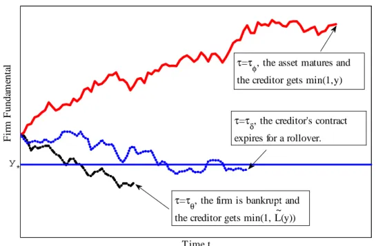
Time t F ir m F unda m enta l y *
τ=τφ, the asset matures and the creditor gets min(1,y)
τ=τδ, the creditor's contract expires for a rollover.
τ=τθ, the firm is bankrupt and the creditor gets min(1, L(y))~
Figure 1: Three possible outcomes to a creditor.
yt (i.e., to roll over if and only if the …rm fundamental is above a threshold). In making his
rollover decision, a creditor rationally anticipates that once he rolls over the debt, he faces the …rm’s rollover risk during his contract period. This is because volatility could cause the …rm fundamental to fall below the other creditors’rollover threshold. As a result, the creditor’s optimal rollover threshold depends on the other creditors’threshold choice.
In this section, we …rst set up an individual creditor’s optimization problem in choosing his optimal threshold. We then construct a unique monotone equilibrium in closed form. Finally, we characterize the key ingredients that lead to the unique equilibrium.
3.1
An Individual Creditor’s Problem
We …rst analyze the optimal rollover decision of an individual creditor who holds a small fraction of the …rm’s outstanding debt. In analyzing the individual creditor’s problem, we take as given that all other creditors use a monotone strategy with a rollover threshold y
(i.e., other creditors will roll over their debt if and only if the …rm fundamental is above y
when their debt contracts mature). During the creditor’s contract period, his value function depends directly on the …rm fundamental yt; and indirectly on the other creditors’rollover
threshold y : Since the creditor’s future payo¤ is proportional to the unit of debt he holds, we denoteV(yt;y ) as the creditor’s value function normalized by the debt unit.
For each unit of debt, the creditor receives a stream of interest payments r until
= min ( ; ; );
which is the earliest of the following three events, illustrated in Figure 1 at the end of three di¤erent fundamental paths. On the top path, the …rm stays alive until its asset matures at . At this time, the creditor gets a …nal payo¤ of min 1; y , i.e., the face value 1 if the asset’s maturity payo¤y is su¢ cient to pay all the debt, andy otherwise. The possibility that the asset’s maturity value may be insu¢ cient to pay o¤ the debt represents the …rm’s insolvency risk. On the bottom path, the …rm fundamental drops below the other creditors’ rollover threshold and the …rm is eventually forced to liquidate its asset prematurely at
. At this time, the creditor gets min (1; L+ly ). This outcome represents the …rm’s rollover risk faced by each creditor. On the middle path, the …rm stays alive (although its fundamental dips below the other creditors’rollover threshold) until when the creditor’s contract expires. At this time, the creditor has an option, i.e., he can choose whether to roll over depending on whether the continuation valueV (y ;y ) is higher than getting the one dollar back.
Due to risk neutrality, the individual creditor’s value function is given by
V (yt;y ) = Et
Z
t
e (s t)rds+e ( t)hmin (1; y )1
f = g (8)
+ min (1; L+ly )1f = g+rollover or runmax fV (y ;y );1g1f = g
io
where 1f g is an indicator function that takes a value of 1 if the statement in the bracket is true or zero otherwise. The individual creditor’s future payo¤ during his contract period depends on other creditors’ rollover choices because other creditors’ runs might force the …rm to liquidate its asset prematurely, as illustrated by the bottom path of Figure 1. This dependence gives rise to strategic complementarity in the creditors’rollover decisions, and therefore a coordination problem between the creditors whose contracts mature at di¤erent times.17
17It is important to note that our model is substantially di¤erent from the standard game theoretical frameworks for analyzing dynamic binary action coordination problems. For example, consider the framework developed in Frankel and Pauzner (2000) and Burdzy, Frankel, and Pauzner (2001). Their framework consists of a sequence of repeated stage games. In each period, each agent receives a ‡ow payo¤, which satis…es an exogenous form of strategic complementarity, i.e., the agent receives a higher ‡ow payo¤ if his current-period strategy overlaps with that of a greater fraction of the population. In contrast, in our model each creditor’s ‡ow payo¤, which is given by the debt contract (interest payment r and possible asset maturity payo¤ min (y;1)), does not exhibit strategic complementarity. Instead, the strategic complementarity between the creditors emerges from the implicit dependence of a creditor’s continuation value function on other creditors’ rollover decisions, as shown in Figure 1 and equation (8). This important di¤erence in model framework
By considering the change of the creditor’s value function over a small time interval
[t; t+dt]; we can derive his Hamilton-Jacobi-Bellman (HJB) equation:
V (yt;y ) = ytVy +
2 2 y
2
tVyy+r+ [min (1; yt) V (yt;y )] (9)
+ 1fyt<y g[min (L+lyt;1) V (yt;y )] + max
rollover or runf0;1 V (yt;y )g:
The left-hand side term V (yt;y )represents the creditor’s required return. This term should
be equal to the expected increment in his value function, as summarized by the terms on the right-hand side.
The …rst two terms ytVy+
2 2 y
2
tVyy capture the expected change in the value function
caused by the ‡uctuation in the …rm fundamental yt:
The third termr is the interest payment per unit of time.
The next three terms capture the three events illustrated in Figure 1:
The fourth term [min (1; yt) V (yt;y )] captures the possibility that the asset
ma-tures during the time interval, which occurs at a probability of dt and generates an impact ofmin (1; yt) V (yt;y )on the creditor’s value function.
The …fth term 1fyt<y g[min (L+lyt;1) V (yt;y )] represents the expected e¤ect
of premature liquidation from other creditors’ runs, which occurs at a probability of 1fyt<y gdt(other maturing creditors will run only ifyt< y ) and generates an impact
of min (L+lyt;1) V (yt;y ) on the creditor’s value function.
The last term max
rollover or runf0;1 V (yt;y )gcaptures the expected e¤ect from the
cred-itor’s own contract expiration, which arrives at a probability of dt: Upon its arrival, the creditor chooses whether to rollover or to run: max
rollover or runf0;1 V (yt;y )g: 18
It is obvious that a maturing creditor will choose to roll over his contract if and only if
V (yt;y ) >1; and to run otherwise. This implies that if the value function V only crosses
1at a single point y0, i.e., V (y0;y ) = 1; then y0 is the creditor’s optimal threshold.
prevents us from readily applying the method of iterated deletion of dominated strategies used by Burdzy, Frankel, and Pauzner (2001) to our model. Instead, we derive the equilibrium by invoking a guess-and-verify approach detailed in the proof of Theorem 1.
18From each creditor’s view, the probability of the event that his contract expires and the …rm is forced into a premature liquidation is in the second order of(dt)2. As a result, whether the creditor gets1 or the asset’s premature liquidation value in such an event is inconsequential. See another related discussion in footnote 16.
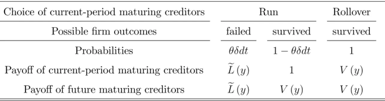
Externality on Future Maturing Creditors The rollover decision of current-period maturing creditors a¤ects not only their own payo¤s, but also future maturing creditors’. In particular, their decision to run adds to the …rm’s bankruptcy probability and thus imposes an implicit cost on future maturing creditors. Since they do not internalize the cost of their actions on others, this externality is the ultimate source of debt runs in our model. To see this point precisely, we summarize the payo¤ (or continuation value) of the current-period maturing creditors and future maturing creditors depending on the choice of the current-period maturing creditors in Table 1. For simplicity, we treat all the current-current-period maturing creditors as one identity in this illustration.
Table 1. Externality on future maturing creditors.
Choice of current-period maturing creditors Run Rollover
Possible …rm outcomes failed survived survived
Probabilities dt 1 dt 1
Payo¤ of current-period maturing creditors Le(y) 1 V (y)
Payo¤ of future maturing creditors Le(y) V (y) V (y)
The maturing creditors will choose run if1 (1 dt)+Le dt > V, which isV <1after ignoring the higher orderdt term. Their runs reduce the remaining creditors’continuation value function by
V hV (1 dt) +Le dti = V Le dt:
While this e¤ect is of the dt order, a remaining creditor needs to bear the accumulative externality e¤ect of all maturing creditors before him, which, in expectation, could be sig-ni…cant.19
Dominance Regions When the …rm fundamentalytis su¢ ciently low (i.e., close to zero),
an individual creditor’s dominant strategy is run. This is because even if all other creditors choose to roll over in the future, the expected asset payo¤ at the maturity plus the interest payments before the asset maturity are not as attractive as getting one dollar back now. On the other hand, when the …rm fundamental yt is su¢ ciently high (i.e., close to in…nity),
the creditor’s dominant strategy is rollover. Even if all other creditors choose to run in the future, the asset’s liquidation value is su¢ cient to pay o¤ the debt in the event of a forced
19Note that the current-period maturing creditors’runs also impose externality e¤ects on each other. But these e¤ects are one time and of thedt order, thus can be ignored.
liquidation. These two regions are called the lower and upper dominance regions. Their existence is important for ensuring a unique equilibrium.
3.2
The Unique Monotone Equilibrium
We …rst focus our attention on symmetric monotone equilibria, and then show that there cannot be any asymmetric monotone equilibrium. In a symmetric monotone equilibrium, each creditor’s optimal threshold choice y0 must be equal to the other creditors’ threshold
y :Thus, we obtain the condition for determining the equilibrium threshold:
V (y ;y ) = 1:
We employ a guess-and-verify approach to derive a unique monotone equilibrium in four steps. First, we derive an individual creditor’s value function V (yt;y ) from the HJB
equation in (9) by assuming that every creditor (including the creditor under consideration) uses the same monotone strategy with a rollover thresholdy . Due to terms min (1; yt) and
min (L+lyt;1)in (9), the value function depends on the value of y in the three cases:
1. If y <1; V(yt;y ) = 8 > > > < > > > : r+ L+ + +(1+ ) + + l + +(1+ ) yt+A1y 1 t when 0< yt y r + + + yt+A2y 2 t +A3yt2 when y < yt 1 r+ + +A4y 2 t when yt>1 ; 2. If 1 y < 1lL; V(yt;y ) = 8 > > > < > > > : r+ L+ + +(1+ ) + + l + +(1+ ) yt+B1y 1 t when0< yt 1 r+ + L+ + +(1+ ) + l + +(1+ ) yt+B2y 1 t +B3yt1 when 1< yt y r+ + +B4y 2 t when yt> y ; 3. If y 1 L l , V (yt;y ) = 8 > > > > > > > < > > > > > > > : r+ L+ + +(1+ ) + + l + +(1+ ) yt+C1y 1 when 0< yt 1 r+ + L+ + +(1+ ) + l + +(1+ ) yt+C2y 1 t +C3yt1 when 1< yt 1lL r+ + + + +(1+ ) +C4y 1 t +C5yt1 when 1lL < yt y r+ + +C6y 2 t when yt> y :
The coe¢ cients 1; 2; 1; 2; A1; A2; A3; A4; B1; B2; B3, B4, C1; C2; C3; C4; C5; and
C6 are given in Appendix A.1 and are expressions of the model parameters and y :
Second, based on the derived value function, we show that there exists a unique …xed pointy such thatV (y ;y ) = 1: Third, we prove the optimality of the threshold y for any individual creditor, i.e.,V(y;y )>1fory > y andV(y;y )<1fory < y :Finally, we show that there cannot be any asymmetric monotone equilibrium.
We summarize the main results in the following theorem.
Theorem 1 There exists a unique monotone equilibrium, in which each maturing creditor
chooses to roll over his debt if yt is above the threshold y and to run otherwise. The
equilibrium threshold y is uniquely determined by the condition that V(y ; y ) = 1.
The equilibrium threshold y could fall into any one of the three cases listed above, depending on the values of the model parameters. The third case is particularly interesting asLe(y ) =L+ly 1;i.e., creditors start to run on the …rm even though the …rm’s current liquidation value is su¢ cient to pay o¤ its liability. The emergence of this type of frantic run re‡ects creditors’strong fear of the …rm’s future rollover risk, which we will discuss in more detail in Section 6.2.
3.3
Understanding the Uniqueness of the Equilibrium
Like the classic bank run model of Diamond and Dybvig (1983), our model also features the externality of one creditor’s run on other creditors. However, there is a unique threshold equilibrium, instead of multiple self-ful…lling equilibria. What leads to the unique equilib-rium? In this section, we discuss the roles of two important ingredients, staggered debt structure and time-varying fundamental, by studying several variations of our model.
3.3.1 Synchronous Debt Expirations
To highlight the role of the staggered debt structure, we consider the following model vari-ation. Suppose that the …rm’s debt contracts all expire at time 0, and the current …rm fundamental isy0. At this time, each creditor decides whether to run or to roll over into a
perpetual debt contract lasting until the …rm asset matures at : We also assume that if all creditors choose to run, the …rm might fail with a probability of s 2 (0;1): This
set-ting closely resembles that in Diamond-Dybvig model, because all creditors simultaneously choose their rollover decisions at time 0 and the …rm does not face any future rollover risk. We formally characterize this coordination problem below.
Proposition 2 Given the aforementioned setting, there existyh > yl >0such that ify0 > yh
(the upper dominance region), an individual creditor’s dominant strategy is to roll over; if
y0 < yl (the lower dominance region), the creditor’s dominant strategy is to run. However, if
y0 2 [yl; yh] (the intermediate region), the creditor’s optimal choice depends on the others’,
i.e., it is optimal to run if the others choose to run and it is optimal to roll over if the others choose to roll over.
Proposition 2 shows that when the …rm fundamental is in an intermediate region, mul-tiple self-ful…lling equilibria emerge, like those in Diamond and Dybvig (1983). By using a staggered debt structure, the …rm can mitigate the Diamond-Dybvig type of coordination problems. This is because the fraction of contracts maturing over a small interval of time (say a day) is small and the collective choice of these creditors is too insigni…cant to a¤ect the …rm. However, there exists another coordination problem between creditors whose contracts mature at di¤erent times. This problem is the core of our model.
3.3.2 Constant Fundamental and Staggered Debt Structure
To highlight the role of the time-varying fundamental, we let the …rm fundamental be con-stant and the …rm have a staggered debt structure. The following proposition shows that in this setting, the coordination problem between creditors whose contracts mature at di¤erent times can still lead to multiple self-ful…lling equilibria.
Proposition 3 Suppose that yt =y is constant (i.e., = 0 and = 0) and the …rm has a
staggered debt structure. There existyc
h > ylc >0such that wheny > yhc (the upper dominance
region), an individual creditor’s dominant strategy is to roll over; when y < yc
l (the lower
dominance region), the creditor’s dominance strategy is to run; and when y 2 [ycl; yhc] (the
intermediate region), the creditor’s optimal choice depends on the others’, i.e., it is optimal to run if the others will choose to run in the future and it is optimal to roll over if the others will choose to roll over in the future.
Proposition 3 shows that when the …rm fundamental is constant and between the upper and lower dominance regions, multiple self-ful…lling equilibria again emerge despite the …rm’s staggered debt structure. In this intermediate region, once each creditor believes that other maturing creditors in the future will all choose to roll over, this “no-future-rollover-risk” belief is self-ful…lling because the …rm fundamental always stays above the lower dominance region and thus will never contradict the no-future-rollover-risk belief. Similarly, once each creditor believes that other maturing creditors in the future will all choose to run, this belief
is also self-ful…lling because the …rm fundamental is always below the upper dominance region.
The staggered debt structure in our model provides a natural debt maturity line for creditors to sequentially withdraw funds from the …rm. This line plays a role similar to the sequential service constraint in the standard bank-run models. In this sense, one can interpret the setting in Proposition 3 as an in…nite-period version of the Diamond-Dybvig model, in which each depositor keeps rolling over term deposits in a bank and the bank fundamental stays constant over time. The emergence of the self-ful…lling bank-run equilibrium in this setting contrasts the …nding of Green and Lin (2003). They consider a …nite-agent version of the Diamond-Dybvig model, and show that the self-ful…lling bank-run equilibrium does not exist under the assumption that the bank’s service line is …nite and each depositor knows his relative position in the line when he contacts the bank. This is because the depositor at the end of the line will rationally choose not to run on the bank, then earlier depositors by backward induction will choose not to run either. This backward induction scheme does not work in our setting. Since the debt maturity line is recurring— i.e., after a creditor rolls over his debt, he goes back to the line— there is not any end of the line to start the backward induction.
3.3.3 Time-Varying Fundamental and Staggered Debt Structure
The self-ful…lling multiple equilibria in Proposition 3 break down if the …rm fundamental changes over time and could reach the upper and lower dominance regions in the future. Instead, a unique (subgame perfect) equilibrium emerges, because anticipation of future creditors’ uniquely determined rollover strategy inside the dominance regions allows the creditors to induce their optimal strategy in the intermediate region between the dominance regions.
It is easy to see this mechanism in the case where the …rm fundamental changes deter-ministically (i.e., = 0 and 6= 0). Suppose that < 0, i.e., the fundamental continues to deteriorate until the asset matures. Knowing that once the fundamental is in the lower dominance region other creditors will always choose run, each maturing creditor right before the fundamental enters the region will choose run. This in turn motivates earlier maturing creditors to choose run too. This backward induction ampli…es the creditors’ incentive to run, and thus generating excessive rollover risk to the …rm. Rollover is optimal only when the current …rm fundamental is su¢ ciently high, i.e., above a threshold y >1; so that it provides enough cushion against the …rm’s future rollover risk. Otherwise, wheny y run is optimal for each creditor. A similar reasoning works in determining a unique equilibrium
for the case >0: The following proposition formally derives this unique equilibrium.
Proposition 4 Suppose that the …rm fundamental is deterministic with a nonzero drift and the …rm has a staggered debt structure.
1. If > 0, there is a unique monotone equilibrium, in which each creditor chooses
rollover if the …rm fundamental is above a threshold y + <1; and run otherwise.
2. If <0, there is a similar unique monotone equilibrium with a threshold y >1.
As a special case of Theorem 1, the same backward induction mechanism also applies to the case where the …rm fundamental is only subject to random shocks (i.e., > 0 and
= 0). That is, random shocks can serve the same role as deterministic drifts, i.e., al-lowing the creditors to backwardly induce the equilibrium in the intermediate region. This key insight follows Frankel and Pauzner (2000) and Burdzy, Frankel, and Pauzner (2001), who show that in dynamic coordination games with strategic complementarities, random fundamental shocks allow agents to coordinate their asynchronous actions and to induce a unique equilibrium. As the realistic debt payo¤s in our model prevent the use of the standard iterated deletion of dominated strategies approach to solve for the equilibrium, our model demonstrates that this insight is robust even in a rather complex and realistic setting.
The emergence of the unique equilibrium in Theorem 1 is analogous to that in the global games models developed by Carlsson and van Damme (1993) and Morris and Shin (1998). In the global games models, agents possess noisy signals about a fundamental variable and each agent uses his private signal to form expectations of other agents’signals and simultaneous actions. In our model, creditors have the same information but make their rollover decisions at di¤erent times. Since the …rm fundamental is time-varying and persistent, the current fundamental allows each maturing creditor to form expectations of future maturing creditors’ rollover decisions.
The following proposition shows that the unique monotone equilibrium derived in The-orem 1 holds even as ! 1; i.e., the maturity of each debt contract converges to zero, just like demand deposits in Diamond and Dybvig (1983).
Proposition 5 When ! 1, the unique equilibrium rollover thresholdy converges to 1lL.
This proposition further shows that it is the asynchronous timing of the creditors’rollover decisions, rather than the non-zero debt maturity, that drives the unique equilibrium in our
model.20 As ! 1; the debt maturity goes down to zero, but the asynchronous timing of the creditors’rollover decisions still remains.21
4
The Single-Creditor Benchmark
To facilitate our discussion of the coordination problem between creditors, it is useful to establish a benchmark case, in which a single creditor holds all the debt of the …rm. Like the main model described in Section 2, we assume that the single creditor faces a contract period which expires upon the arrival of a Poisson shock with intensity . When the contract expires, the single creditor decides whether to roll over the debt for another random contract period or not. If he decides not to roll over, the …rm is forced into a premature liquidation. In this event, the creditor’s payo¤ is min (L+lyt;1). Because the single creditor does not
need to worry about the …rm’s future rollover risk with other creditors, his rollover decision is free of the coordination problem with other creditors. As a result, he would internalize the cost of a premature …rm liquidation. The following proposition shows that he will always roll over his debt if the liquidation cost is su¢ ciently high.
Proposition 6 Suppose that a single creditor …nances all the debt of the …rm. If the cost of
a premature liquidation is su¢ ciently high, i.e., is su¢ ciently low, then the single creditor
will always roll over his debt.
Given that the single creditor will not choose to run in the benchmark case, the runs derived in our main model are ultimately caused by interactions between creditors.
20The …rm’s liquidation value at the limiting running threshold, i.e.,L+ly , is exactly the …rm’s liability 1. When ! 1, each creditor’s contract will mature instantaneously. This means that a creditor will be locked in by his contract only for a short period. However, as other creditors are also kept loose, the …rm could fail at any time if they choose to run. As a result, each creditor will choose to roll over his debt if and only if the …rm’s current liquidation value is su¢ cient to pay o¤ its liability.
21Another special case to consider is when =
1 (i.e., the …rm does not have any credit line.) In this case, the …rm fails immediately if any maturing creditor chooses to run. Because of the frailty of the …rm, the sharing rule between the running creditor and the other creditors during the …rm bankruptcy becomes important. Suppose that the running creditor gets paid in full, while the other creditors divide the liquidation value of the …rm asset. Then, we can show that there is still a unique threshold equilibrium, in which each maturing creditor chooses to run if the fundamental drops below 1 L
l :Deriving this equilibrium follows a similar procedure as outlined in Sections 3.1 and 3.2, except for some minor di¤erences in the formulas. In particular, due to the absence of credit lines, the rollover risk termmin (1; L+ly )1f = g in equation
(8) is replaced by a boundary condition that wheny =y ; V (y; y ) =L+ly : It is direct to see that the equilibrium conditionV(y ; y ) = 1implies thaty = 1lL is the unique equilibrium threshold.
5
Determinants of Equilibrium Rollover Threshold
Despite the absence of self-ful…lling multiple equilibria in our model, preemptive debt runs could still occur through a rat race between the creditors in choosing higher and higher rollover thresholds. In this section, we analyze the e¤ects of this rat race and the dependence of the creditors’ equilibrium rollover threshold on various model parameters, such as the …rm’s liquidation recovery rate , fundamental volatility , and rollover frequency .
For illustration, we will use a set of baseline values for the model parameters:
= 5%; r= 10%; = 10; = 0:2; = 2; = 5%; = 10%; = 60%: (10) The creditors have a discount rate = 5%. The …rm asset generates a constant stream of cash ‡ow at a rate of10%per annum, which is paid out to the creditors as interest payments. The interest payments are attractive since the interest rate r is much higher than the creditors’ discount rate . We choose the …rm’s rollover frequency to be 10, which implies an average debt maturity of about37days (365= ). This implied maturity matches the average maturity of outstanding asset-backed commercial paper in February 2009 (Federal Reserve Release).
= 0:2 implies that the …rm asset on average lasts for 5years (1= ), which is much longer than the debt maturity and resembles the typical duration of a mortgage bond. = 2means that conditional on every maturing creditor choosing to run, the …rm can survive on average for 18 days (1= ).22 The …rm fundamentaly
t has a growth rate of = 5% per annum and
a volatility of = 10% per annum. Finally, when the …rm liquidates its asset prematurely, it only recovers = 60% of the asset’s fundamental value. This implies that L= 0:24 and
l= 0:6in equation (3). Under these baseline parameters, the equilibrium rollover threshold isy = 1:19.
5.1
Liquidation Recovery Rate
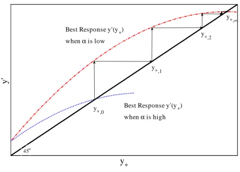
We …rst illustrate the key threshold rat race mechanism using a simple thought experiment. Suppose that initially the liquidation recovery rate of the …rm asset is h; and,
correspond-ingly, every creditor uses an equilibrium threshold levely ;0:Unexpectedly, at a certain time,
all creditors …nd out that the recovery rate drops to a lower level l < h. What would
the new equilibrium threshold be? Let’s start with an individual creditor’s threshold choice, which depends on others’choice. Suppose that all the other creditors still use the original threshold y ;0. Then, by solving the HJB equation in (9), we can derive the creditor’s
op-timal thresholdy ;1;which is higher than y ;0 because the lower liquidation value generates
22This value is rather modest relative to the recent experience of Bear Stearns, which lasted for 3 days under the runs of its creditors and clients before a forced sale to JP Morgan in March 2008, e.g., Cox (2008).
y * y' 45o y *,0 y *,1 y *,2 y *,∞
Best Response y'(y
*)
whenα is high
Best Response y'(y
*)
whenα is low
Figure 2: An illustration of the rat race between creditors in choosing rollover thresholds.
a greater expected loss to the creditor in the event that the …rm is forced into a premature liquidation during his contract period. Of course, each creditor will go through this same calculation and choose a new threshold. If all creditors choose the threshold y ;1, then an
individual creditor’s optimal threshold would be y ;2, another level even higher than y ;1: If
all creditors choosey;2;then each creditor would go through another round of updating, and
so on and so forth. Figure 2 illustrates this updating process until it eventually converges to a …xed pointy ;1, the new equilibrium threshold.
The di¤erence between the threshold levels y ;1 and y;0 represents the necessary safety
margin a creditor would demand in response to the reduced asset liquidation value if other creditors’rollover strategies stay the same. This increase in threshold is eventually ampli…ed to a much larger increasey ;1 y ;0through the rat race between creditors. This ampli…cation
mechanism, which is absent from the single-creditor benchmark, plays a key role in driving the debt runs in our model.
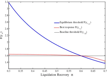
To illustrate the magnitude of this ampli…cation e¤ect, we examine the change in the equilibrium rollover threshold as we vary from its baseline value of 0:6: We measure the threshold by the fundamental value of the …rm asset aty , F(y ) = +r + + y ;which is directly comparable to the …rm’s outstanding liability,1.
In Figure 3, the ‡at thin solid line represents the equilibrium threshold F (y ;0) = 1:59
when takes the baseline value 0:6. The thick solid line shows that as deviates from its baseline value of 0:6 and decreases from 0:7 to 0:3, F (y ;1) rises monotonically from
0.3 0.35 0.4 0.45 0.5 0.55 0.6 0.65 0.7 1.4 1.6 1.8 2 2.2 2.4 2.6 2.8 3 3.2 Liquidation Recovery α F (y * )
Equilibrium threshold F(y*,∞) Best response F(y*,1) Baseline threshold F(y*,0)
Figure 3: The equilibrium rollover threshold vs the liquidation recovery rate : This …gure uses the following baseline parameters: = 5%; r = 0:10; = 10; = 0:2; = 2; = 5%; = 10%;
= 60%: The threshold is measured in the …rm’s fundamental value F(y ): The thin solid line is the baseline threshold level, F(y ;0); under the baseline parameters. The thick solid line plots
the equilibrium thresholdF(y ;1):The dashed line plots a creditor’s best response F(y ;1) to the
change in from its baseline value while …xing the other creditors’threshold atF(y ;0):
1:36 to 3:18: Note that F(y ;1) is always above 1. As each maturing creditor only holds a
partial stake in the …rm, it makes sense for him to run and get his money back before the …rm’s fundamental value drops below the outstanding liability. This is because he does not internalize the cost imposed by his run on the whole …rm.
Moreover, the equilibrium threshold decreases with because a lower liquidation value increases the expected loss to each creditor in the event of a forced liquidation. We formally prove this result in the following proposition:
Proposition 7 The equilibrium rollover threshold y decreases with the …rm’s premature
liquidation recovery rate .
We further decompose F (y ;1) F (y ;0); the e¤ect of an change on F (y ), into two
components. The dashed line in Figure 3 plots the best response of a creditor in the absence of the rat race between creditors. Suppose drops unexpectedly from its baseline level 0:6
to0:4. After the drop in ;by solving the HJB equation in (9) numerically, we …nd that an individual creditor will choose an optimal threshold F(y ;1) = 1:63 (on the dashed line) if
the other creditors’rollover threshold is …xed at the baseline level F(y ;0) = 1:59 (the thin
to compensate the creditor for the increased expected bankruptcy loss in the absence of the rat race. Of course, once we take into account the rat race, each creditor ends up choosing a higher equilibrium threshold of F (y ;1) = 2:38 (on the thick solid line). The di¤erence F(y ;1) F (y ;1)represents the ampli…cation e¤ect of the rat race, which is about20times
the e¤ect without the rat race. Overall, this decomposition shows that in the absence of the rat race between creditors, a change in only has a rather modest e¤ect on each creditor’s threshold choice. However, the rat race dramatically ampli…es this e¤ect on the equilibrium rollover threshold.
5.2
Fundamental Volatility
Fundamental volatility a¤ects an individual creditor’s optimal rollover threshold through several channels. We can intuitively discuss these channels through various terms in the creditor’s value function in equation (8). First, when the …rm’s fundamental volatility in-creases, its insolvency risk, which is re‡ected by the termmin (1; y )1
f = g, rises because
it becomes more likely that the …rm’s asset value at the asset maturity could be insu¢ cient to pay o¤ its liability. The increased insolvency risk prompts each creditor to use a higher rollover threshold. Second, a higher volatility also increases the …rm’s rollover risk through the term min (1; L+ly )1f = g (i.e., other creditors might choose to run and cause the
…rm to fail before the creditor’s debt matures.) More precisely, through a rat race similar to the one described in the previous subsection, imperfect coordination between creditors causes each creditor to choose an even higher threshold to protect himself against other creditors’runs in the future. Third, once the creditor’s debt matures, he has the option to roll over his debt and take advantage of the debt’s high interest payments if the …rm funda-mental is su¢ ciently strong. Through this embedded option, which is re‡ected by the term
maxrollover or runfV (y ;y );1g1f = g;a higher fundamental volatility motivates the creditor
to choose a lower rollover threshold. The e¤ect of the embedded option works in an opposite direction to those of the insolvency risk and rollover risk.
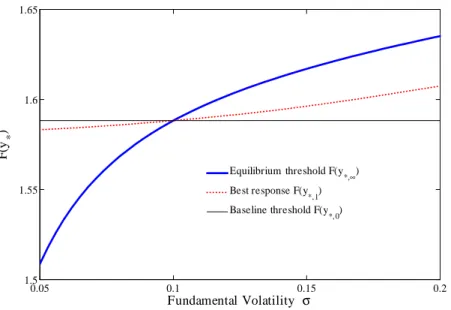
Figure 4 illustrates the net e¤ect of these three channels. As deviates from its baseline value of 10% and increases from 5% to 20%; the creditors’ equilibrium rollover threshold
F(y ) (the thick line) increases from 1:51 to 1:63: We can formally prove that the equilib-rium threshold increases with if the …rm’s credit lines are su¢ ciently unreliable, i.e., is su¢ ciently high. Under this condition, the …rm would easily fail under a run, and con-sequently the embedded-option channel becomes dominated by the other two channels. In fact, our numerical exercises show that this result also holds when takes a modest value.
0.05 0.1 0.15 0.2 1.5 1.55 1.6 1.65 Fundamental Volatility σ F (y * )
Equilibrium threshold F(y
*,∞)
Best response F(y*,1) Baseline threshold F(y
*,0)
Figure 4: The equilibrium rollover threshold vs the fundamental volatility : This …gure uses the following baseline parameters: = 5%; r = 0:10; = 10; = 0:2; = 2; = 5%; = 10%;
= 60%: The threshold is measured in the …rm’s fundamental value F(y ). The thin solid line is the baseline threshold level F(y ;0) under the baseline parameters. The thick solid line plots
the equilibrium thresholdF(y ;1). The dashed line plots a creditor’s best responseF(y ;1) to the
change in from its baseline value while …xing the other creditors’threshold atF(y ;0).
Proposition 8 Suppose that is su¢ ciently high. Then, the equilibrium rollover threshold
y increases with the …rm’s fundamental volatility .
To highlight the e¤ect of the rat race, we also plot an individual creditor’s best response
F(y ;1) to the change in (the dashed line) while …xing the other creditors’ threshold at
the baseline levelF (y ;0) = 1:59when takes its baseline level10%. When rises above its
baseline level, the increase F (y ;1) F (y ;0) represents the safety margin that the creditor
would demand to protect himself against the increased rollover risk in the absence of the rat race between creditors. Note thatF (y ;0)already accounts for the increase in the …rm’s
insolvency risk and the increase in the creditor’s embedded-option value.
As varies from 5% to20%, F (y ;1) increases from1:51to 1:63: Relative to the dashed
line, the thick solid line shows that the range of the equilibrium thresholdF (y ;1)is wider.
For instance, when we increase from10%to15%, an individual creditor will only raise his threshold by0:01; fromF (y ;0) = 1:59 toF (y ;1) = 1:60;if the other creditors’threshold is
…xed at1:59. However, after taking into account the rat race between creditors, each would use a new equilibrium threshold of1:62, which implies that the rat race ampli…es the e¤ect of the volatility increase by 200%.
5 10 15 20 25 30 35 40 45 50 1.15 1.2 1.25 1.3 1.35 1.4 1.45 1.5 1.55 1.6 1.65 Rollover Frequency δ F (y * )
Equilibrium threshold F(y
*,∞)
Best response F(y*,1) Baseline threshold F(y
*,0)
Figure 5: The equilibrium rollover threshold vs the rollover frequency : This …gure uses the following baseline parameters: = 5%; r = 0:10; = 10; = 0:2; = 2; = 5%; = 10%;
= 60%: The threshold is measured in the …rm’s fundamental value F(y ): The thin solid line is the baseline threshold level F(y ;0) under the baseline parameters. The thick solid line plots
the equilibrium thresholdF(y ;1). The dashed line plots a creditor’s best responseF(y ;1) to the
change in from its baseline value while …xing the other creditors’threshold atF(y ;0).
5.3
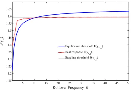
Rollover Frequency
The …rm’s rollover frequency is another key determinant of its rollover risk. As increases, each creditor’s contract period, which has an expected duration of 1= ; gets shorter. This generates two opposing e¤ects on the equilibrium. First, each individual creditor is locked in for a shorter period. As a result, his embedded option on the …rm is more valuable as he has more ‡exibility to pull out if the …rm fundamental deteriorates. The increased embedded-option value makes the creditor more willing to roll over his debt, i.e., to choose a lower rollover threshold. On the other hand, a higher also means that the other creditors are locked in for a shorter period. As a result, during the creditor’s contract period, the …rm is more susceptible to the rollover risk created by the other creditors. The increased rollover risk therefore motivates him to choose a higher rollover threshold. The equilibrium threshold
y trades o¤ the embedded-option e¤ect and the rollover-risk e¤ect.
Figure 5 plots the equilibrium rollover threshold (the thick solid line) as we vary from its baseline value of 10 to a range between 0:2 to 50, along with an individual creditor’s best response (the dashed line) to the change while …xing the other creditors’ rollover threshold at the baseline level of1:59. As increases from0:2to50;the equilibrium rollover