ISSN 2042-2695
CEP Discussion Paper No 1289
August 2014
The Latin American Efficiency Gap
Francesco Caselli
Abstract
The average Latin American country produces about 1 fifth of the output per worker of the US. What are the sources of these enormous income gaps? I report development-accounting results for Latin America. On average Latin America’s overall physical and human capital endowment relative to the USA is essentially identical to Latin America’s efficiency relative to the USA . In my main sample average relative capital and average relative efficiency are both roughly double actual average relative incomes. Hence, both capital gaps and efficiency gaps are very large: the average Latin American country has less than half the capital (human and physical) per worker of the US, and uses it less than half as efficiently. In assessing this evidence, it is essential to bear in mind that efficiency gaps contribute to income disparity both directly -- as they mean that Latin America gets less out of its capital -- and indirectly -- since much of the capital gap itself is likely due to diminished incentives to invest in equipment, structure, schooling, and health caused by low efficiency. The consequences of closing the efficiency gap would correspondingly be far reaching. Explaining the Latin American efficiency gap is therefore a high priority both for scholars and for policy makers.
Key words: Latin America, income gaps, development accounting JEL: O11
This paper was produced as part of the Centre’s Macro Programme. The Centre for Economic Performance is financed by the Economic and Social Research Council.
This paper is part of a research project on Latin American and Caribbean convergence financed by the Latin American and Caribbean Region of the World Bank. I am very grateful to Federico Rossi for excellent research assistance, to Ludger Woessman for patient and constructive advice, and to Jorge Araujo and the other participants in the project for helpful comments.
Francesco Caselli is the Macro Programme’s Director at the Centre for Economic Performance, London School of Economics and Political Science. He is also Norman Sosnow Professor of Economics at LSE.
Published by
Centre for Economic Performance
London School of Economics and Political Science Houghton Street
London WC2A 2AE
All rights reserved. No part of this publication may be reproduced, stored in a retrieval system or transmitted in any form or by any means without the prior permission in writing of the publisher nor be issued to the public or circulated in any form other than that in which it is published.
Requests for permission to reproduce any article or part of the Working Paper should be sent to the editor at the above address.
F. Caselli, submitted 2014.
1
Introduction
The average Latin American country produces about 1 …fth of the output per worker of the US. What are the sources of these enormous income gaps? This paper reports development-accounting results for Latin America. Development accounting compares di¤erences in income per worker between developing and developed countries to counter-factual di¤erences attributable to observable components of physical and human capital. Such calculations can serve a useful preliminary diagnostic role before engaging in deeper and more detailed explorations of the fundamental determinants of di¤erences in income per worker. If di¤erences in physical and human capital –orcapital gaps –are su¢ cient to explain most of the di¤erence in incomes, then researchers and policy makers need to focus on factors holding back investment (in machines and in humans). Instead, if di¤erences in capital are insu¢ cient to account for most of the variation in income, one must conclude that developing countries are also hampered by relatively low e¢ ciency at using their inputs - e¢ ciency gaps. The research and policy agenda would then have to focus on technology, allocative e¢ ciency, competition, and other determinants of the e¢ cient use of capital.1
1For a detailed exposition of development accounting see, among others, Caselli (2005).
I present development-accounting results for 2005 for three samples of Latin American countries: a “broad”sample of 22 countries, a “narrow”sample of 9, and an “intermediate” sample of 15.
The three samples di¤er in the data available to measure human capital. In the broad sample human capital is measured in the context of a “Mincerian” framework, where the key inputs are schooling (years of education) and health (as proxied by the adult survival rate). In the narrow and intermediate samples I augment the Mincerian framework with measures of cognitive skills, to account for additional factors such as schooling quality, parental inputs, and other in‡uences on human capital not captured by years of schooling and health. The measures of cognitive skills are based on tests administered to school-age children. In the narrow sample, the test is a science test whose results are directly compa-rable between Latin America and the benchmark developed country. In the intermediate sample the tests were only administered in Latin America and can be compared to the benchmark country only on the basis of a number of ad hoc assumptions.
In all three samples I measure physical capital as an aggregate of reproducible and “natural” capital. Reproducible capital includes equipment and structures, while natural capital primarily includes subsoil resources, arable land, and timber.
Given measures of physical capital gaps, as well gaps in the components of human capital, development-accounting uses a calibration to map these gaps into counter-factual income gaps, or the income gaps that would be observed based on di¤erences in human and capital endowments only. Because these counterfactual incomes are bundles of physical and human capital, I refer to the ratio of Latin American counterfactual incomes to the US counterfactual income asrelative capital.
For each of the three samples I present results from two alternative calibrations, a “baseline”calibration and an “aggressive”calibration. The baseline calibration makes use of the existing body of microeconomic estimates of the Mincerian framework in the way that
most closely …ts the theoretical framework of development accounting. As it turns out, this leads to coe¢ cients for the components of human capital that are substantially lower than in much existing work in development accounting - leading to relatively smaller estimated capital gaps and, correspondingly, larger e¢ ciency gaps. The aggressive calibration thus uses more conventional …gures as a robustness check.
When I use my benchmark calibration, irrespective of sample/cognitive skill correction, I …nd that relative capital and relative e¢ ciencies are almost identical. For example in the broad sample average relative capital and average relative e¢ ciency are both 44% - or roughly double actual average relative incomes. Hence, both capital gaps and e¢ ciency gaps are very large: the average Latin American country has less than half the capital (human and physical) per worker of the US, and uses it less than half as e¢ ciently.
Using the aggressive calibration, capital gaps are naturally larger, and e¢ ciency gaps correspondingly smaller. Nevertheless, even under this “best-case scenario” for the view that capital gaps are the key source of income gaps, average Latin American e¢ ciency is at most 60% of the US level, still implying a vast e¢ ciency gap.
In assessing this evidence, it is essential to bear in mind that e¢ ciency gaps contribute to income disparity both directly – as they mean that Latin America gets less out of its capital – and indirectly – since much of the capital gap itself is likely due to diminished incentives to invest in equipment, structure, schooling, and health caused by low e¢ ciency. The consequences of closing the e¢ ciency gap would correspondingly be far reaching.
Explaining the Latin American e¢ ciency gap is therefore a high priority both for schol-ars and for policy makers. It is likely that this task will require …rm-level evidence. Firm level evidence would also be invaluable in checking the robustness of the development-accounting results, which are subject to severe data-quality limitations.
2
Conceptual Framework
The analytical tool at the core of development accounting is the aggregate production func-tion. The aggregate production function maps aggregate input quantities into output. The main inputs considered are physical capital and human capital. The empirical literature so far has failed to uncover compelling evidence that aggregate input quantities deliver
large external economies, so it is usually deemed safe to assume constant returns to scale.2 Given this assumption, one can express the production function in intensive form, i.e. by specifying all input and output quantities in per worker terms. In order to construct coun-terfactual incomes a functional form is needed. Existing evidence suggests that the share of capital in income does not vary systematically with the level of development, or with factor endowments [Gollin (2002)]. Hence, most practitioners of development accounting opt for a Cobb-Douglas speci…cation. In sum, the production function for countryi is
yi =Aikih
1
i ; (1)
where y is output per worker, k is physical capital per worker, h is human capital per worker (quality-adjusted labor), and A captures unmeasured/unobservable factors that contribute to di¤erences in output per worker.
The termAis subject to much speculation and controversy. Practitioners refer to it as total factor productivity, technology, a measure of our ignorance, etc. Here I will refer to it as “e¢ ciency”. Countries with a largerA are countries that, for whatever reasons, are more e¢ cient users of their physical and human capital.
The goal of development accounting is to assess the relative importance of e¢ ciency di¤erences and physical and human capital di¤erences in producing the di¤erences in income per worker we observe in the data. To this end, one constructs counterfactual incomes, or capital bundles,
~
yi =kih
1
i ; (2)
which are based exclusively on the observable inputs. Di¤erences in these capital bundles are then compared to income di¤erences. If counter-factual and actual income di¤erences are similar, then observable factors are able to account for the bulk of the variation in income. If they are quite di¤erent, then di¤erences in e¢ ciency are important. Establishing how signi…cant e¢ ciency di¤erences are has important repercussions both for research and for policy.
2See, e.g. Iranzo and Peri (2009) for a recent review and some new evidence on the quantitative
In order to construct the counterfactual y~s we need to construct measures of ki and
hi, as well as to calibrate the capital-share parameter . Standard practice sets the latter
to 0.33, and we stick to this practice throughout. Caselli (2005) shows that development-accounting calculations are not overly sensitive to alternative values in a reasonable range. The rest of this section focuses on the measurement of physical and human capital.3
Existing development-accounting calculations measure k exclusively on the basis of
reproducible capital (equipment and structures). But in most developing countries, where agricultural and mining activities still represent large shares of GDP, natural capital (land, timber, ores, etc.) is also very important. Caselli and Feyrer (2007) show that omitting natural capital can lead to very signi…cant understatements of total capital in developing countries relative to developed ones. Hence, this study will measure k as the sum of the value of all reproducible and natural capital.
Human capital per worker can vary across countries as a result of di¤erences in knowl-edge, skills, health, etc. The literature has identi…ed three variables that vary across countries which may capture signi…cant di¤erences in these dimensions: years of schooling [e.g., Klenow and Rodriguez-Clare (1997), Hall and Jones (1999)], health [Weil (2007)], and cognitive skills [e.g. Hanushek and Woessmann (2012a)]. In order to bring these together, we postulate the following model for human capital:
hi = exp( ssi+ rri+ tti): (3)
In this equation, si measures average years of schooling in the working-age population,
ri is a measure of health in the population, and ti is a measure of cognitive skills. The
coe¢ cients s, r, and t map di¤erences in the corresponding variables into di¤erences in human capital.4
The model in (3) is attractive because it o¤ers a strategy for calibration of the
para-3There may well be signi…cant heterogeneity among Latin American countries, and, more importantly,
between Latin America and the benchmark rich country, in the value of . However, it is not known how
to perform development-accounting with country-speci…c capital shares. This is because measures of the capital stock are indices, so that a requirement for the exercise to make sense is that the results should be
invariants to the units in whichkis measured. Now(ki=kj) is unit-invariant, but kii=k
j
j is not.
meters s, r, and t. In particular, combining (1), (3), and an assumption of perfect
competition in labor markets, we obtain the “Mincerian” formulation
log(wij) = i+ ssij + rrij+ ttij; (4)
where wij (sij; etc.) is the wage (years of schooling, etc.) of worker j in country i, and i is a country-speci…c term. This suggests that using within-country variation in wages,
schooling, health, and cognitive skills one might in principle identify the coe¢ cients . In practice, there are severe limitations in following this strategy, that we discuss after introducing the data.
3
Data
We work with three samples, broad, narrow, and intermediate. The broad data set contains all Latin American countries for which we have data fory,k,s, andr, all observed in 2005. There are 22 such countries (excluded are Barbados, Cuba, and Paraguay, for which we have no capital data). The other two samples add alternative measures oft. The trade-o¤ is that one measure o¤ers a more credible comparison with the benchmark high-income country, but is only available for 9 Latin-American economies. The more dubious but more plentiful measure is available for 15 countries. All but one of the countries in the narrow sample are also in the intermediate sample (Trinidad and Tobago is the exception). The dataset also includes data from the USA, which we use as the benchmark rich country.
Per-worker income yi is variable rgdpwok from version 7.1 of the Penn World Tables
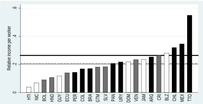
(PWT71). Figure 1 shows per-worker income in each country in the broad sample relative to the USA, oryi=yU S. Countries that are also included in the narrow sample are in black,
and countries that are in the intermediate but not the narrow sample are in grey. With the exception of Trinidad and Tobago, all Latin America countries have per-worker incomes
is considerable micro and macro evidence against the assumption that workers wiith di¤erent years of schooling are perfect substitutes [e.g. Caselli and Coleman (2006)]. In this paper I abstract from the issue of imperfect substitutability. Caselli and Ciccone (2013) argue that consideration of imperfect substitution is unlikely to reduce the estimated importance of e¢ ciency gaps.
Figure 1: Income per worker relative to the US 0 .2 .4 .6 R el ativ e i nco me p er wo rk er H TI N IC
BOL HND GUY ECU PER COL BRA GTM SLV PAN URY DOM VEN JAM ARG CRI BLZ CHL MEX TTO
White bars; only broad sample. Grey bars: only broad and intermediate samples. Black bars: all samples (except TTO not in intermediate). Dashed line: broad sample mean. Light solid line: intermediate sample mean. Heavy solid line: narrow sample mean. Source: PWT71.
well below 40% of the US level, sometimes much below. The horizontal lines show the three (unweighted) sample averages, indicating that the average country is only one …fth as productive as the USA.5
World Bank (2012) presents cross-sectional estimates of the total capital stock, k, as well as its components, for various years. The total capital stock includes reproducible capital, but also land, timber, mineral deposits, and other items that are not included in standard national-account-based data sets. The basic strategy of the World Bank team that constructed these data begins with estimates of the rental ‡ows accruing from di¤erent types of natural capital, which are then capitalized using …xed discount rates. I construct the total capital measure by adding the variables producedplusurban and natcap.
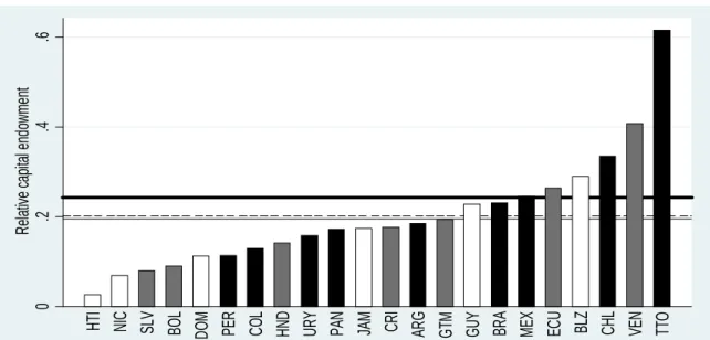
Figure 2 shows total (reproducible plus natural) capital per worker estimates for Latin American countries relative to the US, ki=kU S. The average Latin American worker is
endowed with approximately one …fth of the physical capital of the average US worker.
5In the narrow sample the average is higher due to the disproportionate weight of Trinidad and Tobago.
Figure 2: Physical capital per worker relative to the US 0 .2 .4 .6 R el ativ e ca pi tal end ow me nt H TI N IC
SLV BOL DOM PER COL HND URY PAN JAM CRI ARG GTM GUY BRA MEX ECU BLZ CHL VEN TTO
White bars; only broad sample. Grey bars: only broad and intermediate samples. Black bars: all samples (except TTO not in intermediate). Dashed line: broad sample mean. Light solid line: intermediate sample mean. Heavy solid line: narrow sample mean. Source: World Bank (2012).
For average years of schooling in the working-age population (which is de…ned as be-tween 15 and 99 years of age) I rely on Barro and Lee (2013). Note from equation (3) that for the purposes of constructingrelative human capitalhi=hU S what is relevant is the
di¤erence in years of schoolingsi sU S. The same will be true forr andt. Accordingly, in
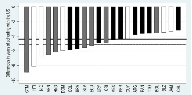
Figure 3 I plot schooling-year di¤erences with the USA in 2005. Latin American workers have always at least three year less schooling than American ones, and …ve on average.
As a proxy for the health status of the population, r, Weil (2007) proposes using the adult survival rate. The adult survival rate is a statistic computed from age-speci…c mortality rates at a point in time. It can be interpreted as the probability of reaching the age of 60, conditional on having reached the age of 15, at current rates of age-speci…c mortality. Since most mortality before age 60 is due to illness, the adult survival rate is a reasonably good proxy for the overall health status of the population at a given point in time. Relative to more direct measures of health, the advantage of the adult survival rate is that it is available for a large cross-section of countries. I construct the adult survival rate from the World Bank’s World Development Indicators. Speci…cally, this is the weighted average of male and female survival rates, weighted by the male and female share in the population.
Figure 3: Di¤erences in years of schooling with the US -10 -8 -6 -4 -2 0 Di ffere nce s i n y ears of s cho ol in g wi th the US G TM HTI NIC VEN HND DOM OLC BRA SLV ECU URY CRI
MEX PER GUY ARG PAN TTO BOL BLZ JAM CHL
White bars; only broad sample. Grey bars: only broad and intermediate samples. Black bars: all samples (except TTO not in intermediate). Dashed line: broad sample mean. Light solid line: intermediate sample mean. Heavy solid line: narrow sample mean. Source: Barro and Lee (2013).
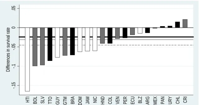
In Figure 4 I plot adult survival rate di¤erences with the USA. Survival rate probabil-ities are lower in Latin America than in the US, but perhaps not vastly so. On average, Latin American 15-year olds are only 4 percentage points less likely to reach the age of 60 than US 15-year olds.6
Following work by Gundlach, Rudman, and Woessman (2002), Woessman (2003), Jones and Schneider (2010) and Hanushek and Woessmann (particularly 2012a), we also wish to account for di¤erences in cognitive skills not already accounted for by years of schooling and health. The ideal measure would be a test of average cognitive ability in the working population. Hanushek and Zhang (2009) report estimates of one such test for a dozen countries, the International Adult Literacy Survey (IALS), but only one of these is in Latin America (Chile).
As a fallback, I rely on internationally comparable test scores taken by school-age children. In the narrow sample, I will use scores from a science test administered in 2009
Figure 4: Di¤erences in survival rate with the US -.15 -.1 -.05 0 .05 D iffe ren ces in sur vi val ra te H TI
BOL SLV TTO GUY GTM BRA DOM JAM NIC HND OLC VEN PER ECU BLZ RGA MEX PAN URY CHL CRI
White bars; only broad sample. Grey bars: only broad and intermediate samples. Black bars: all samples (except TTO not in intermediate). Dashed line: broad sample mean. Light solid line: intermediate sample mean. Heavy solid line: narrow sample mean. Source: WDI.
to 15 year olds by PISA (Program for International Student Assessment). There are in principle several other internationally-comparable tests (by subject matter, year of testing, and organization testing) that could be used in alternative to or in combination with the 2009 PISA science test. However there would be virtually no gain in country coverage by using or combining with other years (the PISA tests of 2009 are the ones with the greatest participation, and virtually no Latin American country participated in other worldwide tests and not in the 2009 PISA tests).7 Focusing only on one test bypasses potentially thorny issues of aggregation across years, subjects, and methods of administration. Cross-country correlations in test results are very high anyway, and very stable over time.8 Data on PISA test score results are from the World Bank’s Education Statistics.
Aside from the world-wide tests of cognitive skills used in the narrow sample, there are
7The only exception is Belize, which participated in some of the reading tests admninistered by PIRLS
(Progress in International Reading Literacy Study).
8Repeating all my calculations using the PISA math scores yielded results that were virtually
also two “regional”tests of cognitive skills that have been administered to a group of Latin American countries: the …rst in 1997 by the Laboratorio Latinoamericano de Evaluación de la Calidad de la Educación (LLECE), covering reading and math in the third and fourth grade; the second in 2006 by the Latin American bureau of the UNESCO, covering the same subjects in third and sixth grade. These tests are described in greater detail in, e.g., Hanushek and Woessman (2012a), who also argue that these tests may better re‡ectwithin Latin-American di¤erences in cognitive skills.
From the perspective of this study, the main attraction of these alternative measures of cognitive skills is that they cover a signi…cantly larger sample. The biggest problem, of course, is that they exclude the United States (or any high-income country) and so, on the face of it, they are unusable for constructing counterfactual relative incomes. However, Hanushek and Woessman (2012a) propose a methodology to “splice” the regional scores into their worldwide sample. While this splicing involves a large number of assumptions that are di¢ cult to evaluate, it is worthwhile to assess the robustness of my results to these data.9
Needless to say measuring t by the above-described test scores is clearly very unsatis-factory, as in most cases the tests re‡ect the cognitive skills of individuals who have not joined the labor force as of 2005, much less those of the average worker. The average Latin American worker in 2005 was 36 years old, so to capture their cognitive skills we would need test scores from 1984.10 Implicitly, then, we are interpreting test-score gaps in current children as proxies for test scores gaps in current workers. If Latin America and the US have experienced di¤erent trends in cognitive skills of children since 1984 this assumption is problematic.
The 2009 PISA science tests are reported on a scale from 0 to 1000, and they are nor-malized so that the average scoreamong OECD countries (i.e. among all pupils taking the test in this set of countries) is (approximately) 500 and the standard deviation is
(approxi-9Hanushek and Woessman (2012a) splice the regional scores into world-wide scores that are themselves
aggregates of multiple waves and multiple subject areas - obtained with a methodology described in Hanushek and Woessman (2012b).
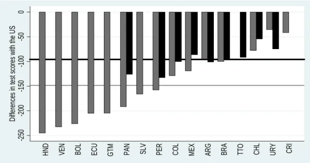
Figure 5: Di¤erences in test scores with the US -2 50 -2 00 -1 50 -1 00 -50 0 D iffe ren ces in te st sc or es wi th the U S H ND VEN BOL E CU G TM PAN SLV PER COL MEX ARG BRA TTO CHL URY CRI
Grey bars: regional test/intermediate sample. Black bars: PISA test/narrow sample. Light solid line: regional-test mean. Heavy solid line: PISA-test mean. Source: World Bank’s Education Statistics and Hanushek and Woessman (2012a, 2012b).
mately) 100.11 The regional scores are put on the PISA scale by Hanushek and Woessman’s splicing, so they can be directly compared. Figure 5 shows test score di¤erences ti tU S
for the narrow and intermediate samples. Di¤erences in PISA scores are very signi…cant: the average Latin American student in 2009 shows cognitive skills that are below those of his US counterpart by about one standard deviation of the OECD distribution of cog-nitive skills. Only Chile is a partial stand-out, with a cogcog-nitive gap closer to one half of one standard deviation. Di¤erences in Hanushek and Woessman’s spliced regional tests are even more signi…cant, with the average gap exceeding 1.5 standard deviations. Recall that the PISA scores are directly comparable between Latin American and USA, while
11I say approximately in parenthesis because the normalization was applied to the 2006 wave of the
test. The 2009 test was graded to be comparable to the 2006 one. Hence, it is likely that the 2009 mean (standard deviation) will have drifted somewhat away from 500 (100) - though probably not by much. The PISA math and reading tests were normalized in 2000 and 2003, respectively, so their mean and standard deviation are more likely to have drifted away from the initial benchmark. This is one reason why I use the science test for my baseline calculations.
the spliced regional tests – while arguably giving a more accurate sense of within Latin America di¤erences –are less suitable for poor country-rich country comparisons. Hence, the discrepancy in cognitive-skill gaps between the PISA and the regional scores implies that the latter should be treated with caution.
4
Calibration
The last, and most di¢ cult, step in producing counter-factual income gaps between US and Latin America is to calibrate the coe¢ cients s, r, and t. As discussed, equation (4) indicates that, using within country data on w, s, r, and t, one could in principle identify these coe¢ cients by running an extended Mincerian regression for log-wages. In implementing this plan, we are confronted with (at least) two important problems.
The …rst problem is that one of the explanatory variables, the adult survival rate
r, by de…nition does not vary within countries. Estimating r directly is therefore a
logical impossibility. To solve this problem Weil (2007) notices that, in the time series (for a sample of ten countries for which the necessary data is available), there is a fairly tight relationship between the adult survival rate and average height. In other words, he postulatesci = c+ cri, whereci is average height and the coe¢ cient c is estimated from
the above-mentioned time series relation (he obtains a coe¢ cient of 19.2 in his preferred speci…cation). Since height does vary within countries as well as between countries, this opens the way to identifying r by means of the Mincerian regression
log(wij) = i+ ssij + ccij + ttij;
where r = c c.12
The second problem is that measures of t are not consistent at the macro and at the micro level. In particular, while we do have micro data sets reporting both results from tests of cognitive skills and wages, the test in question is simply a di¤erent test from the tests we have available at the level of the cross-section of countries. Call the alternative test
12Needless to say if we had cross-country data on average height there would be no need to use the
available at the micro level d. Once again the solution is to assume a linear relationship
di = dti. The di¤erence with the case of height-survival rate is that, as far as I know, there
is no way to check the empirical plausibility of this assumption. Given the assumed linear relationship, one can back out d as the ratio of the within country standard deviation of
dij and tij. With d at hand, one can back out t from the modi…ed Mincerian regression
log(wij) = i+ ssij + ccij + ddij; (5)
using t = d d.
In choosing values for s, c, and dfrom the literature it is highly desirable to focus on
microeconomic estimates of equation (5) that include all three right-hand variables. This is becauses,c, andd are well-known to be highly positively correlated.13 Hence, any OLS estimate of one of the coe¢ cients from a regression that omits one or two of the other two variables will be biased upward.14
A search of the literature yielded one and only one study reporting all three coe¢ cients from equation (5). Vogl (2014) uses the two waves (2002 and 2005) of the nationally-representative Mexican Family Life Survey to estimate (5) on a subsample of men aged 25-65. In his study, w is measured as hourly earnings, s as years of schooling, c is in centimeters, and d is the respondent’s score on a cognitive-skill test administered at the time of the survey.15 The cognitive skill measure is scaled so its standard deviation in the Mexican population is 1.16
The coe¢ cients reported by Vogl are as follows (see his Table 4, column 7). The return to schooling s is 0.072, which can be plugged directly in equation (3). The “return to
height” c is 0.013. Hence, the coe¢ cient associated with the adult survival rate in (3)
13See, e.g., the literature review in Vogl (2014).
14An alternative would be to use IV estimates of the s, but instruments for the variables on the right
hand side of equation 5 are often somewhat controversial - especially for height and cognitive skills.
15The test is the short-form Raven’s Progressive Matrices Test.
16Needless to say there are aspects of Vogl’s treatment that imply the regressions he runs are not a
perfect …t for the conceptual framework of the paper. It may have been preferable for our pusposes to include both men and women. He also controls for ethnicity, age, and age squared, which do not feature in my framework. Finally, he notes that the Raven’s core is a coarse measure of cognitive skills, giving raise to concerns with attenuation bias (more on this below).
is 0.013 x 19.2 = 0.25, where I have used Weil’s mapping between height and the adult survival rate. Finally, the reported return to cognitive skills dis 0.011. Since the standard deviation ofdis one by construction, and the standard deviation of the 2009 Science PISA test in Mexico is 77, the implied coe¢ cient on the PISA test for the purposes of constructing
h is 0.011/77=0.00014.17
The coe¢ cients in my baseline calibration are considerably lower than those used in other development-accounting exercises. For schooling, applications usually gravitate to-wards the “modal” Mincerian coe¢ cient of 0.10. For the adult survival rate, Weil (2007) uses 0.65, on the basis of considerably higher estimates of the returns to height than those reported by Vogl. For the return to cognitive skills, Hanushek and Woessmann (2012a) advocate 0.002, which is more than one order of magnitude larger than the value I derive from the Vogl’s estimates.18
The fact that the parameters calibrated on Vogl’s estimates are smaller than those commonly used is consistent with the discussion above. In particular, the alternative estimates are often based on regressions that omit one or two of the variables in (5), and are therefore upward biased. Another consideration is that there is considerable cross-country heterogeneity in the estimates, and that researchers often focus on estimates from the USA, which are often larger.19;20
17Hanushek and Woessman’s splicing procedure implies that the same coe¢ cient can be used for the
regional tests used in the intermediate sample.In particular, the relevant standard error is the average of the standard deviations of Pisa science and math tests in Mexico, which is 80. Then we have 0.011/80 = 0.00014.
18This is based on Hanushek and Zhang (2009), who use the International Adult Literacy Survey (IALS)
to estimate the return to cognitive skills in a set of 13 countries. The value of 0.002 is the one for the USA.
19For example, in Hanushek and Zhang (2009), the estimated market return to cognitive skills varies
(from minimum to maximum) by a factor of 10! The estimate from the USA, which is used in Hanushek
and Woessman (2012a) is themaximum of this distribution.
20This is actually an issue with the capital share as well. However, the issue there is less severe as
observed capital shares do not vary systematically withy, so it should be possible to ascribe the observed
variation to measurement error. In other words the patterns of variation in do not necessarily rise the
On the other hand, Vogl’s regressions are admittedly estimated via OLS, and there is a real concern with attenuation bias from measurement error. In order to gauge the sensitivity of my results to possibly excessively low values of the calibration parameters due to attenuation bias, I will also present results based on an “aggressive” calibration, which uses a Mincerian return of 0.10, Weil’s 0.65 value for the mapping of the adult survival rate to human capital, and Hanushek and Woessman’s 0.002 coe¢ cient on the PISA test.21
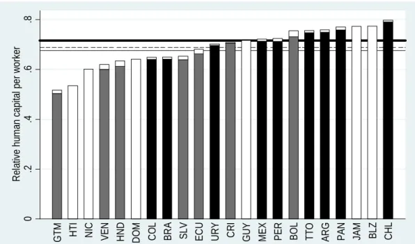
Figure 6: Human capital per worker relative to the US - baseline calibration
0 .2 .4 .6 .8 R el ativ e h um an ca pi tal pe r wo rk er G TM HTI NIC VEN HND OMD COL BRA SLV ECU U RY CRI
GUY MEX PER BOL TTO ARG PAN JAM BLZ CHL
Overall height: relative human capital per worker without cognitive-skill correction. Grey (Black) bars: relative human capital per worker with cognitive-skill correction based on regional (PISA) tests. Dashed line: average with no cognitive-skill correction. Light (heavy) solid line: average with regional-(PISA-)test correction.
Figure 6 shows human-capital per worker estimates for Latin American countries rel-ative to the US, hi=hU S, under my baseline calibration. The full height of the bar shows
21As described above the Hanushek and Zhang estimate for the US comes from a testddi¤erent fromt.
In order to go from their coe¢ cient d to the coe¢ cient of interest twe need to multiply the former by
the ratio of the standard deviation ofdU S;i to the standard deviation oftU S;i. Since Hanushek and Zhang
standardize the variabled, we just have to multiply by the inverse of the standard deviation oftU S;i. But
in the test we are using this is just 0.98, so the correction would be immaterial.I use the same value both in the narrow and in the intermediate sample.
the value of hi=hU S when excluding cognitive skills, and is thus fully comparable across
all countries in the …gure. The solid bars are the values when including cognitive skills. Irrespective of sample and cognitive-skill correction the average Latin American worker is endowed with approximately 70% of the human capital of the average US worker.
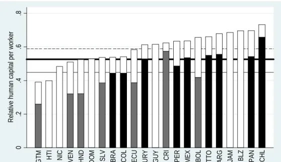
Figure 7: Human capital per worker relative to the US - aggressive calibration
0 .2 .4 .6 .8 R el ativ e h um an ca pi tal pe r wo rk er G TM HTI NIC VEN HND OMD SLV BRA COL ECU U RY GUY C RI
PER MEX BOL TTO ARG JAM BLZ PAN CHL
Overall height: relative human capital per worker without cognitive-skill correction. Grey (Black) bars: relative human capital per worker with cognitive-skill correction based on regional (PISA) tests. Dashed line: average with no cognitive-skill correction. Light (heavy) solid line: average with regional-(PISA-)test correction.
Figure 7 is analogous to Figure 6 but shows the aggressive calibration instead. Not Surprisingly, using the aggressive calibration results in signi…cantly lower relative human capital for Latin America, since the impact of di¤erentials in schooling, health, and cogni-tive skills is magni…ed. Human capital gaps become particularly large when including the cognitive-skill corrections.
5
Results
5.1
Baseline Calibration
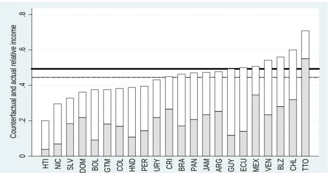
In the large sample we lack cognitive skill information for more than half of the countries, so we set t = 0. Figure 8 shows each country’s counterfactual income relative to the US (relative capital) in 2005, y~i=y~U S, as well as the relative incomes yi=yU S already shown in
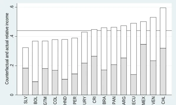
Figure 8: Relative capital, baseline calibration, no cognitive-skill correction 0 .2 .4 .6 .8 Co un te rfa ct ua l an d act ua l r ela tive in com e H TI N IC S LV D OM BOL GTM COL H ND PER U RY CRI B RA PAN JAM A RG GUY ECU
MEX VEN BLZ CHL TTO Overall height: relative capital per worker. Grey bars: relative income per worker. Dashed line: broad sample mean. Light solid line: intermediate sample mean. Heavy solid line: narrow sample mean.
Figure 1. In particular, for each country the overall height of the bar is relative capital, while the height of the shaded bar is relative income.
As is apparent, there is a lot of variation in relative capital, ranging from 20% to almost 70%. This re‡ects considerable heterogeneity in rates of physical and human-capital accumulation among Latin American countries, as seen above. Sample means are between 44% (broad and intermediate sample) and 49% (narrow sample). This means that observed distributions of physical and human capital are consistent with Latin American workers being between 44 and 49% as productive as USA ones. We can interpret this measure as a measure of the capital gap between Latin America and the US.
In Figure 9 we extend our calculations to include information on cognitive skills based on worldwide PISA test scores. The sample size correspondingly drops to 9 countries. The e¤ect of including cognitive skills under my baseline calibration is virtually nil: the mean remains unchanged at 0.49. This result is expected given the very small calibrated “loading” on cognitive skills implied by Vogl’s estimates. Very similar patterns emerge when using the regional scores/intermediate sample, as seen in Figure 10.
Figure 9: Relative capital, baseline calibration, PISA cognitve skills 0 .2 .4 .6 .8 Co un te rf act ua l an d act ua l r ela tive in com e C OL
PER URY BRA PAN ARG MEX CHL TTO
Overall height: relative capital per worker. Grey bars: relative income per worker. Solid line: mean.
5.2
“Aggressive” Calibration
My baseline calibration uses coe¢ cients for mapping years of schooling, health, and cog-nitive skills into human capital that, taken individually, are lower than those presented in other contributions. In this section I explore the robustness to my results to more commonly-used values. Hence, I set s= 0:10, r = 0:65, and t = 0:002.
Results from the large sample using this aggressive calibration are shown in Figure 11. Given the larger coe¢ cients, counterfactual incomes are necessarily smaller than under the baseline calibration. Yet quantitatively the di¤erence is not very large. Average relative capital drops to 40%, so still roughly double relative income.
Figure 12 shows the results from the aggressive calibration using the PISA test scores. Including cognitive skills in the calculation of relative capital has a much bigger impact than under the baseline, because the coe¢ cient on cognitive skills is an order of magnitude larger. The average counterfactual relative income falls to 40%, compared with 49% in the baseline calibration (within the same narrow sample). This is a large gain in explanatory power of observables. For many countries, the gap between relative income and relative capital shrinks considerably.
Figure 10: Relative capital, baseline calibration, “regional-test” cognitive skills 0 .2 .4 .6 Co un te rf a ct ua l an d act ua l r e la tive in com e S LV
BOL GTM COL HND PER URY RIC BRA PAN ARG ECU MEX VEN CHL
Overall height: relative capital per worker. Grey bars: relative income per worker. Solid line: mean.
regional test scores. Recall that these tests tend to show even larger cognitive gaps with the US. Correspondingly, using these tests in combination with the aggressive calibration leads to an even better alignment between relative capital and relative income.
6
Implications for E¢ ciency Gaps
We have seen that, depending on cognitive skill correction, counterfactual income ratios (relative capital) in Latin America tend to be much larger than actual income ratios. This discrepancy implies that Latin America su¤ers from ane¢ ciency gap as much as it su¤ers from a capital gap.
We can quantify e¢ ciency gaps by noting, from (1) and (2), that
Ai AU S = yi=yU S ~ yi=y~U S :
Hence, Latin American e¢ ciency gaps can be directly gleaned from Figures (8)-(13) by simply dividing the height of the shaded bars by the overall height of the bars.
In Table 1 I report the sample averages of the implied e¢ ciency gaps, for the vari-ous cognitive skill correction - calibration combinations. For completeness I also report
Figure 11: Relative capital, aggressive calibration, no cognitive-skill correction 0 .2 .4 .6 Co un te rf act ua l an d act ua l r ela tive in com e H TI N IC S LV G TM D
OM COL HND BOL PER URY BRA CRI JAM PAN
A
RG GUY ECU
MEX VEN BLZ CHL TTO
Overall height: relative capital per worker. Grey bars: relative income per worker. Dashed line: broad sample mean. Light solid line: intermediate sample mean. Heavy solid line: narrow sample mean.
the corresponding averages for relative income and relative capital, as well as labor-force weighted means.
Using the baseline calibration, average relative capital and average relative e¢ ciency are almost identical, irrespective of sample/cognitive skill correction/weighting. One way to put this is that capital gaps and e¢ ciency gaps contribute equally to Latin American income gaps. When using the aggressive calibration, the relative importance of capital gaps increases, particularly when adding the cognitive-skill corrections. Still, even under the most aggressive scenario average Latin American relative e¢ ciency is only 60% of US e¢ ciency.22
In order to fully appreciate the importance of these e¢ ciency gaps it is crucial to note that, under almost any imaginable set of circumstances, physical (speci…cally, reproducible) and human capital accumulation respond to a country’s level of e¢ ciency. The higher A
22In the narrow sample it is probably best to focus on the labor-force weighted results, as the unweighted
Figure 12: Relative capital, aggressive calibration, PISA cognitive skills 0 .2 .4 .6 Co un te rf act ua l an d act ua l r ela tive in com e C OL
PER URY BRA PAN ARG MEX CHL TTO
Overall height: relative capital per worker. Grey bars: relative income per worker. Solid line: mean.
the higher the marginal productivity of capital, leading to enhanced incentives to invest in equipment and structure, schooling, etc. While quantifying this e¤ect is di¢ cult, most theoretical frameworks would lead one to expect it to be large. Hence, it is legitimate to conjecture that a signi…cant fraction of the capital gap may be due to the e¢ ciency gap.23
7
Implications and Conclusions
There is a large gap in income per worker between Latin America and the USA: Latin American workers are only about one …fth as productive as workers from the United States. A development-accounting calculation reveals that both capital gaps and e¢ ciency gaps contribute to this overall productivity gap. In particular, a Cobb-Douglas aggregate
23In principle, one might also argue for a reverse direction of causation, with larger physical and
human-capital stocks leading to higher e¢ ciency. In particular, this would be true if the model was misspeci…ed, and there were large externalities. But as already mentioned the empirical literature has not to date uncovered signi…cant evidence of externalities in physical and human capital.
Figure 13: Relative capital, aggressive calibration, “regional-test” cognitive skills 0 .1 .2 .3 .4 .5 Co un te rf a ct ua l an d act ua l r e la tive in com e S LV G TM H ND BOL C OL
PER PAN ECU VEN BRA URY C
RI
A
RG
MEX CHL
Overall height: relative capital per worker. Grey bars: relative income per worker. Solid line: mean.
of observable physical and human capital per worker is roughly in the order of 40% on average of the corresponding US level (capital gap) – implying that the e¢ ciency with which inputs are used in Latin America is in the order of 50% of US levels (e¢ ciency gap). Reducing this e¢ ciency gap would reduce the overall productivity gap both directly, by allowing Latin America to reap greater bene…ts from its physical and human capital, and indirectly, since much of the capital gap is likely due to the e¢ ciency gap itself: closing the e¢ ciency gap would stimulate investment at rates potentially capable of closing the capital gap as well.
These conclusions are contingent on the quality of the underlying macroeconomic data. There is growing concern about the quality and reliability of the PPP national-account …gures in the Penn World Tables and similar data sets [e.g. Johnson et al. (2013)]. Similar concerns apply, no doubt, to our proxies for human capital as well (as already discussed particularly in the context of cognitive skills). It is true that such concerns are most often voiced in the context of implied comparisons of changes, especially over short time spans: cross-country comparisons of levels reveal such gigantic di¤erences (as seen above) that they seem unlikely to be entirely dominated by noise. Still, exclusive reliance on these macro data is highly inadvisable.
Table 1: Summary of Results
Calibration
Baseline Aggressive
Sample/Cognitive Skill Measure Relative Relative Relative Relative Relative GDP Capital E¢ ciency Capital E¢ ciency
Broad/None 0.21 0.44 0.44 0.40 0.49 0.21 0.46 0.45 0.41 0.50 Narrow/PISA 0.26 0.49 0.52 0.40 0.64 0.22 0.46 0.47 0.37 0.59 Intermediate/“Regional” 0.20 0.44 0.45 0.33 0.60 0.22 0.46 0.46 0.36 0.60
Bold entries are unweighted sample means. Plain entries are labor-force weighted sample means
Fortunately, it is also increasingly unnecessary. The increasing availability of …rm level data sets, particularly when matched with employee-level information (e.g. about schooling), provides an opportunity to supplement the macro picture with microeconomic productivity estimates comparable across countries.
The bene…t of producing such micro productivity estimates is by no means limited to permitting to check the robustness of conclusions concerning average capital and e¢ ciency gaps - though this bene…t alone is su¢ cient to make such exercises worthwhile. An ad-ditional bene…t is to uncover information on the within country distribution of physical capital, human capital, and e¢ ciency. A relatively concentrated distribution would sug-gest that e¢ ciency gaps are mostly due to aggregate, macroeconomic factors that a¤ect all …rms fairly equally (e.g. impediment to technology di¤usion from other countries). A very dispersed distribution, with some …rms close to the world technology frontier, would be more consistent with allocative frictions that prevent capital and labor to ‡ow to the more e¢ cient/talented managers.
More generally, …rm-level data is likely to prove essential in the quest for the determi-nants of the large e¢ ciency gaps revealed by the development-accounting calculation. After all, (in-)e¢ ciency is –by de…nition –a …rm-level phenomenon. Most of the most plausible
possible explanations for the e¢ ciency gap are microeconomic in nature – whether it is about …rms unable to adapt technologies developed in more technologically-advanced coun-tries, failures in the market for managers and/or capital, frictions in the matching process for workers, etc. It seems implausible that evidence for or against these mechanisms can be found in the macro data. Yet understanding the sources of the Latin American e¢ ciency gap is unquestionably the most urgent task for those who want to design policies aimed at closing the Latin American income gap.
References
Barro and Lee (2013): "A New Data Set of Educational Attainment in the World, 1950-2010."Journal of Development Economics.
Caselli, F. (2005): “Accounting for cross-Country Income Di¤erences,” in Philippe Aghion and Stephen Durlauf (eds.),Handbook of Economic Growth, Volume 1A, 679-741, Elsevier.
Caselli, Francesco, and Antonio Ciccone (2013): “The Contribution of Schooling in Development Accounting: Results from a Nonparametric Upper Bound.”Journal of De-velopment Economics.
Caselli, Francesco and Coleman, John Wilbur II, 2006. "The World Technology Fron-tier." American Economic Review, 96, pp. 499-522.
Caselli, Francesco, and James Feyrer, 2007. "The Marginal Product of Capital." Quar-terly Journal of Economics, 122, pp. 535-568.
Gollin, Douglas, 2002. "Getting Income Shares Right." Journal of Political Economy, 110, pp. 458-474.
Gundlach, Rudman, and Woessman (2002): “Second Thougths on Development Ac-counting,”Applied Economics, 34, 1359-69.
Hall, Robert and Charles Jones, 1999. "Why Do Some Countries Produce So Much More Output Per Worker Than Others?" Quarterly Journal of Economics, 114, pp. 83-116 Hanusheck, Eric, and Ludger Woessman (2012a): "Schooling, Educational Achieve-ment, and the Latin American Growth Puzzle", Journal of Development Economics 99 (2), 497-512,
Hanushek, Eric A.,Woessmann, Ludger, (2012b). Do better schools lead to more growth? Cognitive skills, economic outcomes, and causation. Journal of Economic Growth. Hanushek, Eric and Lei Zhang (2009): “Quality-Consistent Estimates of International Schooling and Skill Gradients,”Journal of Human Capital, 2009, 3(2), 107-43.
Iranzo, Susana and Giovanni Peri, 2009. "Schooling Externalities, Technology, and Productivity: Theory and Evidence from US States." Review of Economics and Statistics, 91, pp. 420-431
Johnson, Simon, William Larson, Chris Papageorgiou, and Arvind Subramanian (2013): “Is Newer Better? Penn World Table Revisions and Their Impact on Growth Estimates,”
Journal of Monetary Economics, March 2013.
Klenow, Peter, and Andres Rodriguez-Claire, 1997. "The Neoclassical Revival in Growth Economics: Has It Gone Too Far?". In NBER Macroeconomic Annual, MIT Press
Vogl, Tom S. (2014): “Height, Skills, and labor market outcomes in Mexico,”Journal of Development Economics, 107, 84-96.
Weil, David, 2007. “Accounting for the E¤ect of Health on Economic Growth.”Quarterly Journal of Economics, 122, pp.1265-1306.
Woessman, Rudiger (2003): “Specifying Human Capital,”Journal of Economic Sur-veys, 17, 3, 239-270.
CENTRE FOR ECONOMIC PERFORMANCE Recent Discussion Papers
1288 Thomas Sampson Dynamic Selection: An Idea Flows Theory of
Entry, Trade and Growth 1287 Fabrice Defever
Alejandro Riaño
Gone for Good? Subsidies with Export Share Requirements in China: 2002-2013
1286 Paul Dolan
Matteo M. Galizzi
Because I'm Worth It: A Lab-Field Experiment on the Spillover Effects of Incentives in Health
1285 Swati Dhingra Reconciling Observed Tariffs and the Median
Voter Model 1284 Brian Bell
Anna Bindler Stephen Machin
Crime Scars: Recessions and the Making of Career Criminals
1283 Alex Bryson
Arnaud Chevalier
What Happens When Employers are Free to Discriminate? Evidence from the English Barclays Premier Fantasy Football League 1282 Christos Genakos
Tommaso Valletti
Evaluating a Decade of Mobile Termination Rate Regulation
1281 Hannes Schwandt Wealth Shocks and Health Outcomes:
Evidence from Stock Market Fluctuations 1280 Stephan E. Maurer
Andrei V. Potlogea
Fueling the Gender Gap? Oil and Women's Labor and Marriage Market Outcomes 1279 Petri Böckerman Alex Bryson Jutta Viinikainen Christian Hakulinen Laura Pulkki-Raback Olli Raitakari
Biomarkers and Long-term Labour Market Outcomes: The Case of Creatine
1278 Thiemo Fetzer Fracking Growth
1277 Stephen J. Redding Matthew A. Turner
Transportation Costs and the Spatial Organization of Economic Activity
1276 Stephen Hansen Michael McMahon Andrea Prat
Transparency and Deliberation within the FOMC: A Computational Linguistics Approach
1275 Aleksi Aaltonen Stephan Seiler
Quantifying Spillovers in Open Source Content Production: Evidence from Wikipedia
1274 Chiara Criscuolo Peter N. Gal Carlo Menon
The Dynamics of Employment Growth: New Evidence from 18 Countries
1273 Pablo Fajgelbaum Stephen J. Redding
External Integration, Structural
Transformation and Economic Development: Evidence From Argentina 1870-1914
1272 Alex Bryson
John Forth Lucy Stokes
Are Firms Paying More For Performance?
1271 Alex Bryson
Michael White
Not So Dissatisfied After All? The Impact of Union Coverage on Job Satisfaction
1270 Cait Lamberton
Jan-Emmanuel De Neve Michael I. Norton
Eliciting Taxpayer Preferences Increases Tax Compliance
1269 Francisco Costa Jason Garred João Paulo Pessoa
Winners and Losers from a Commodities-for-Manufactures Trade Boom
1268 Seçil Hülya Danakol Saul Estrin
Paul Reynolds Utz Weitzel
Foreign Direct Investment and Domestic Entrepreneurship: Blessing or Curse?
1267 Nattavudh Powdthavee Mark Wooden
What Can Life Satisfaction Data Tell Us About Discrimination Against Sexual
Minorities? A Structural Equation Model for Australia and the United Kingdom
1266 Dennis Novy
Alan M. Taylor
Trade and Uncertainty
1265 Tobias Kretschmer Christian Peukert
Video Killed the Radio Star? Online Music Videos and Digital Music Sales
The Centre for Economic Performance Publications Unit Tel 020 7955 7673 Fax 020 7404 0612