Three Essays on Credit Risk Models and Their Bayesian Estimation

Three Essays on Credit Risk Models and Their Bayesian

Estimation

(Article begins on next page)

The Harvard community has made this article openly available.

Please share

how this access benefits you. Your story matters.

Citation

Kwon, Tae Yeon. 2012. Three Essays on Credit Risk Models and

_{Their Bayesian Estimation. Doctoral dissertation, Harvard}

University.

Accessed

April 17, 2018 3:41:54 PM EDT

Citable Link

http://nrs.harvard.edu/urn-3:HUL.InstRepos:9288549

Terms of Use

This article was downloaded from Harvard University's DASH

_{repository, and is made available under the terms and conditions}

applicable to Other Posted Material, as set forth at

http://nrs.harvard.edu/urn-3:HUL.InstRepos:dash.current.terms-of-use#LAA

c

⃝2012 - Tae Yeon Kwon

Dissertation Advisors: Professor Stephen Blyth Tae Yeon Kwon

Three Essays on Credit Risk Models and Their Bayesian Estimation

ABSTRACT

This dissertation consists of three essays on credit risk models and their Bayesian estimation. In each essay, defaults or default correlation models are built under one of two main streams in credit risk model study: the structural and the intensity models. The first essay studies the usefulness and methods to combine multiple securities information in a single firm asset process and to estimate its parameters under the structural model. The second essay investigates multi-firm correlated defaults, with special focus on industry-specific correlation under the intensity model. The third essay studies the use of multiple securities information to estimate the multi-firm correlated defaults model under both structural and intensity models.

In our first essay, sequential estimation on hidden asset value and model parameters estima-tion are implemented under the Black-Cox model. To capture short-term autocorrelaestima-tion in the stock market, we assume that market noise follows a mean reverting process. For estimation, two Bayesian methods are applied in this essay: the particle filter algorithm for sequential estimation of asset value and the generalized Gibbs sampling method for model parameters estimation. The first simulation study shows that sequential hidden asset value estimation using option price and equity price is more efficient and accurate than estimation using only equity price. The second simulation study shows that by applying the generalized Gibbs sampling method, model param-eters can be successfully estimated under the model setting that there is no closed-form solution. In an empirical analysis using eight companies, half of which are DowJones30 companies and the other half non-Dow Jones 30 companies, the stock market noise for the firms with more liquid stock is estimated as having smaller volatility in market noise processes.

In our second essay, the frailtyidea described in Duffie, Eckner, Horel, and Saita (2009) is expanded to industry-specific terms. The MCEM algorithm is used to estimate parameters and

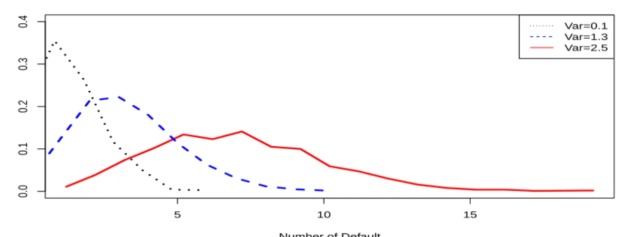
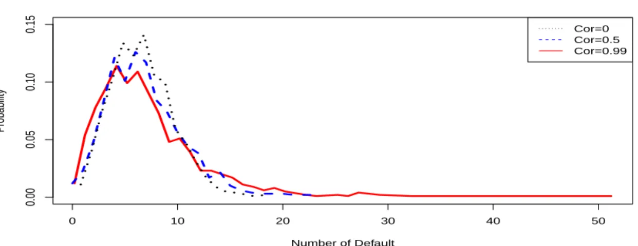
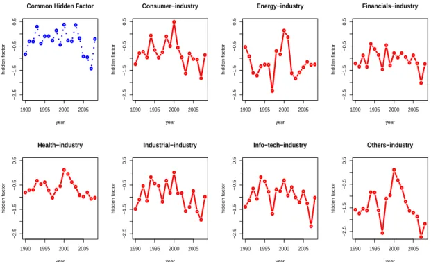
random effect processes under the condition of unknown hidden paths and analytically-difficult likelihood functions. The estimate used in the study are based on U.S. public firms between 1990 and 2008. By introducing industry-specific hidden factors and assuming that they are random effects, a comparison is made of the relative scale of within- and between-industries correlations. A comparison study is also developed among a without-hidden-factor model, a common-hidden-factor model, and our industry-specific common-common-hidden-factor model. The empirical results show that an industry-specific common factor is necessary for adjusting over- or under-estimation of default probabilities and over- or under-estimation of observed common factor effects.

Our third essay combines and extends works of the first two essays by proposing a com-mon model frame for both structural and intensity credit risk models. The comcom-mon model frame combines the merits of several default correlation studies which are independently developed under each model setting. Following the work of Duffie, Eckner, Horel, and Saita (2009), we apply not only observed common factors, but also un-observed hidden factor to explain the cor-related defaults. Bayesian techniques are used for estimation and generalized Gibbs sampling and Metropolis-Hasting (MH) algorithms are developed. More than a simple combination of two model approaches (structural and intensity models), we relax the assumptions of equal factor ef-fect across entire firms in previous studies, instead adopting a random coefficients model. Also, a novelty of the approach lies in the fact that CDS and equity prices are used together for estima-tion. A simulation study shows that the posterior convergence is improved by adding CDS prices in estimation. Empirical results based on daily data of 125 companies comprising CDS.NA.IG13 in 2009 supports the necessity of such relaxations of assumption in previous studies. In order to demonstrate potential practical applications of the proposed framework, we derive the posterior distribution of CDX tranche prices. Our correlated structural model is successfully able to predict all the CDX tranche prices, but our correlated intensity model results suggests the need for further modification of the model.

TABLE OF CONTENTS

Abstract . . . . iii

Acknowledgments . . . . viii

0. Background and Motivation . . . . 1

1. Structural Credit Risk Model When Market Prices Are Contaminated with Noise . . . . 6

1.1 Introduction . . . 6

1.2 The Model . . . 9

1.2.1 Basic Model: Equity Prices in the Presence of Market Noise . . . 9

1.2.2 Multiple Asset Class : Pricing Options on Equity . . . 13

1.3 The Sequential Estimation on Hidden Asset Process . . . 15

1.3.1 Estimation Procedure . . . 15

1.3.2 Simulation-Based Result . . . 17

1.4 Parameter Estimation . . . 20

1.4.1 Simple Gibbs Sampling Method . . . 20

1.4.2 Generalized Gibbs Sampling: Scale Transformation Update . . . 23

1.4.3 Simulation Studies . . . 24

1.5 Empirical Analysis . . . 29

1.6 Conclusion . . . 31

2. Industry-Specific Correlated Defaults . . . . 33

2.1 Introduction . . . 33

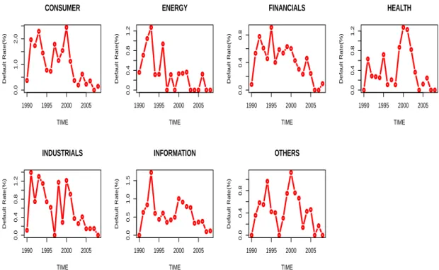
2.2 Data: Default and Industry . . . 37

2.2.1 Data Overview . . . 37

2.2.2 Industry Categories . . . 38

2.2.3 Defaults in Each Industry . . . 39

2.3 Model . . . 41

2.3.1 Mixed Effect Model with Correlated Industry-Specific Default Intensity . 41 2.3.2 Observed Factors:Ui,t,Xt . . . 43

2.3.3 Hidden Factor (Yj,t) . . . 44

2.4 Properties of the Model: Correlation Structure . . . 45

2.4.1 Model for Industry Hidden Effects . . . 46

2.4.2 Within- and Between-Industry Correlation . . . 47

2.5 Estimation . . . 50

2.6 Empirical Results . . . 52

2.6.2 Estimated Random Effect: ˆK, ˆΣ . . . 53

2.7 Model Comparison . . . 54

2.7.1 Comparison of Estimated Observed Factor Effect and Hidden Factor . . . 54

2.7.2 Comparison of Estimated Default Distribution . . . 57

2.8 Conclusion . . . 61

3. Parallel Intensity and Structural Models for Correlated Defaults . . . . 63

3.1 Introduction . . . 63

3.2 Background in Finance . . . 66

3.2.1 Credit Risk Model and Default Correlation Studies . . . 66

3.2.2 CDS Market . . . 68

3.3 Preliminary Study: Variables and Model Structure Selection . . . 70

3.3.1 Variables (Observed Factors) Selection . . . 70

3.3.2 Random Coefficients . . . 72

3.3.3 Random Time Effect (Hidden Factor) . . . 73

3.4 Overview of the Models . . . 75

3.5 Model 1: Correlated Structural Model . . . 76

3.5.1 State Level: Correlated Asset Model . . . 76

3.5.2 Observation Level: Pricing Function of Equity and CDS Prices . . . 78

3.5.3 Properties of the Model . . . 82

3.6 Model 2 : Correlated Intensity Model . . . 83

3.6.1 State Level : Correlated Intensity Model . . . 83

3.6.2 Observation Level : Pricing Function of CDS Spread . . . 84

3.6.3 Properties of the Model . . . 86

3.7 Estimation . . . 86

3.7.1 Estimation Procedure for Model 1: Correlated Structural Model . . . 87

3.7.2 Estimation Procedure for Model 2: Correlated Intensity Model . . . 90

3.8 Simulation . . . 91

3.8.1 Simulation Result for Model 1: Correlated Structural Model . . . 91

3.8.2 Simulation Result for Model 2: Correlated Intensity Model . . . 94

3.9 Data and Calibration . . . 97

3.9.1 Data Overview . . . 97

3.9.2 Calibration of Default Barrier and Recovery Rate . . . 99

3.10 Empirical Results . . . 100

3.10.1 Empirical Results for Model 1: Correlated Structural Model . . . 100

3.10.2 Empirical Results for Model 2: Correlated Intensity Model . . . 108

3.11 Pricing CDS Index Tranches Prices . . . 112

3.12 Conclusion . . . 119

Appendix 123 A. Appendices to Chapter 1 . . . . 124

A.1 Bond Price under the Black-Cox Model . . . 124

B. Appendices to Chapter 3 . . . . 127

B.1 The Posterior Scale Reduction Factor . . . 127

B.1.1 The Convergence of Model 1 . . . 127

B.1.2 The Convergence of Model 2 . . . 128

B.2 More Simulation Results . . . 129

B.2.1 More Simulation Results for Model 1 . . . 129

B.2.2 More Simulation Results for Model 2 . . . 131

B.3 Summary of 108 Companies in the Sample . . . 132

B.4 More Empirical Results . . . 135

B.4.1 More Empirical Results for Model 1. . . 135

B.4.2 More Empirical Results for Model 2. . . 138

B.5 More Results on CDX Tranche Pricing . . . 141

ACKNOWLEDGMENTS

I am deeply grateful for the guidance of my thesis committee: Yoonjung Lee, Stephen Blyth, Tirthankar Dasgupta and Xiao-Li Meng. I acknowledge helpful comments from Steven Finch and Samuel Kou.

Most importantly, I thank my husband, my daughter, and my parents for their love and en-couragement. I could not have written this without their support. This dissertation is dedicated to them.

0. BACKGROUND AND MOTIVATION

In the financial market, numerous and various market prices of financial securities are ob-served. Given these market prices, many investors and financial analysts ask a critical question, namely, what are market perceptions in the context of default probabilities? To answer this, re-search in the area of credit risk modeling has evolved by building a better statistical model de-scribing defaults and trying to deduce prices from these models. The research in this dissertation is one such effort.

The literature in the credit risk area attempts to describe the default processes of debt as be-ing primarily based on one of two types of models: the structural model or the intensity model. In this dissertation, we also expand models under one of these two types; therefore the general background and motivation for our three essays will first be introduced.

Structural models price corporate debts and equity as contingent claims on the underlying asset value of a firm. When the asset value of the firm falls below a certain threshold, the firm fails to meet its obligations to the debt holders, thus triggering a default event. The Merton model (Merton (1974)) provides a fundamental framework for various other structural models. The main idea behind Merton’s model is to consider equity as a European-call-option-type contingent claim on asset. Black and Cox (Black and Cox (1976)) base their model on Merton’s model, but they relax their assumption of default time.

Unlike structural models, intensity models specify neither firm value processes nor default boundaries explicitly. Defaults are instead modeled as stochastic events whose arrival rates are governed by the given intensities. The parameters governing intensities are typically assumed to depend on a set of market data.

market price. The prices observed in the financial market are numerous and various due to the large number of firms issuing multiple securities. Studies in this dissertation develop from single firm to multi-firm and from single security to multiple securities. Our study on default modeling starts from the multiple securities issued by a single firm which is described in Chapter 1. We then extend to multi-firms defaults analysis using the information of one security in Chapter 2. Finally, in Chapter 3, we combine all works in previous two research and then analyze multi-firm defaults using multiple securities.

The first essay conducted here is a cross-asset class research project with the consideration of each market noise based on the Black-Cox structural model. Structural models, in general, have potential advantages over intensity models in cross-asset class research. Conceptually, the capital structure of a firm can be evaluated as a whole in one consistent framework by structural models. Subsequently, methodologies for estimating models in a structural setting may deliver enhanced performances, since the relevant information can be pooled from the financial markets for other asset classes.

However, the default study based on a single-firm always has limitations in terms of default correlation. In the simplest case, default correlation is caused if one firm is a creditor of another. But primarily, and more generally, it is because the health of individual companies are linked together via industry-specific and/or general economic conditions.(see Lucas (1995), Zhou (2001)) The historical data also shows that all companies suffer or prosper together. For example, the pattern of yearly default rate for all U.S. corporate debt since 1900 shows the high concentration of defaults around 1914 and 1933. Many firms defaulted in those two depressions. All businesses tend to be adversely affected at the same time, because of their sensitivity to the general economy. (Lucas (1995))

Conversely, the default of one company can have an impact on other companies or general economic conditions. For example, during 2001, the year when Enron defaulted, the NASDAQ index fell 74% from its high and 171 large corporations declared bankruptcy, which was two times more than what took place in 2000. Bankruptcies were common throughout 2002, continuing into July, 2002 when WorldCom, the countrys second largest long-distance telecom company,

filed for bankruptcy(Smith and Walter (2006)). During the financial crisis that started in 2007, many financial institutions collapsed and finally in September, 2008 Lehman Brothers declared bankruptcy. However a more serious problem is that the impact of the bankruptcy of Lehman Brothers is not just constrained in the U.S. The fall of Lehman Brothers resulted in a 3.2% dip in the U.S. GDP within a span of six months, between the third quarter of 2008 and first quarter of 2009. The effect of the Lehman Brothers default in Italy, EU-27, Germany, and U.K. was even worse; these countries experienced a 4.4%, 4.1%, 5.8%, and 3.5% drop, respectively, during this period (see Daveri (2009)). Based on the fact that the U.S. GDP growth rate during the first six months in 2008 was only +1.14%, these rate drops were considered quite serious. This economic downturn brought by one firm’s default might again affect the default risk of other firms.

From our second essay, we steer our study to multi-firm defaults analysis from the single firm default analysis. The key issues of the multi-firm defaults study is to find a way to capture default correlations more accurately. In practice, understanding default correlation correctly is important for understanding the distribution of a loan portfolio’s loss and risk management. Particularly, in markets such as synthetic collateralized debt obligations (CDO), which are heavily reliant on the market for default swaps and often have basket structures, a modeling default correlation is necessary for pricing and rating. For example, the higher the correlation, the smaller the gap between the estimated risk of a CDO’s AAA tranche and its equity tranche.

As our first multi-firm study, we build a model for correlated defaults under the intensity model in our second essay. The reason for switching to the intensity model from the structural model is because under the intensity model default correlation can be measured more easily by assuming commonly shared factors. As Duffie and Garleanu (2001), the intensity model assume that the default intensities of all firms are conditionally independent given the path of the state. The intensity model evolves by relaxing this conditional independent assumption. Collin-Dufresne and Helwege (2003) relax the conditional independence assumption, allowing default intensities to depend also on a common unobserved factor. In their model, a market-wise response to a credit event is due to investors’ updating their beliefs about the unobserved factor after encountering a credit event. More recently, Duffie, Eckner, Horel, and Saita (2009) implement an intensity model

with a common unobserved factor namedfrailty. In our second essay, we expand thisfrailtyidea to industry-specific terms and build the model under more relaxed assumptions allowing all different within-and between-industries correlations.

Finally, in our third essay, we extend previous studies in both directions: the multiple securities and the multiple firms. In terms of the multiple securities study, a typical structural model has an advantage. However, a typical intensity model has a merit in dealing with multi-firms. Therefore, we propose multi-firms defaults model frames and an estimation method using the multiple secu-rities information under both intensity and structural credit risk model within the parallel model frame. We combine advantages and ideas in previous studies of intensity and structural correlated defaults models, then build one common structure for both. As a combining work of two different credit risk model studies, the main contribution of our third essay is that by proposing a common model structure for both structural and intensity models, we are able to compare the two under fair conditions. The relative importance of hidden common factors is compared to observed com-mon factors in both models. Furthermore, a comparison is made of the performance of the CDX tranche price prediction between the two models.

However, as a first step in combining the work of two different credit risk model studies, we need to simplify some important points already suggested in our previous two essays. Even though we simplify the model with a common hidden factor instead of the industry-specific factors (proposed in the second essay), and we assume independent normal trading noise in the stock and CDS markets instead of mean-reverting process (proposed in the first essay), our third essay can be interpreted as synthesizing the work in our first two essays. We will leave relaxing such constraints as our future works.

Detailed statistical estimation methodologies adopted in each essay is different, but they all belong to the category of Bayesian analysis. The Bayesian approach is adaptable to cases where a closed-form solution is unavailable. Prediction is the other reason for using the Bayesian ap-proach. By adopting the Bayesian method, we are able to extract more information on the hidden asset or intensity value itself as well as various financial securities. Because the Bayesian ap-proach produces the posterior distribution of unknown parameters instead of one single value of

estimates, the distribution of a future observation known as a posterior predictive distribution can be easily derived. Furthermore, not only are the distribution of hidden asset or intensity values and prices used for estimation, but also the distribution of other securities not used in the estimation procedure, are all available.

1. STRUCTURAL CREDIT RISK MODEL WHEN MARKET PRICES ARE CONTAMINATED WITH NOISE

1.1

Introduction

Since Black and Scholes (1973) and Merton (1974) first considered equity as a call option on the firm’s asset value, Merton’s structural model has remained as the basic reference in pricing defaultable bonds. The major difficulty of the structural approach is that the firm’s asset value is not observed directly. Through the observable equity prices, we are able to infer about the hidden asset values. However, since observed equity value is often contaminated by trading noise, arriving at inference becomes complicated. Faced with these challenges, this essay presents two types of estimation procedures of the Black and Cox model within a Bayesian framework. In the sense of cross-asset class research, sequential estimation of hidden asset value process is conducted first under the condition that all parameters are given. We then propose the method for estimation of all model parameters and asset processes together.

The contributions of this essay can be summarized as follows: First, we allow for trading noises in the observed equity prices, which follow a mean-reverting process. In markets where the trading noise effect exists, it will be ill-advised to ignore its presence. In recent years, research on trading noise has provided reasons for this fact. For instance, Ait-Sahalia and Zhang (2005a) analyze the effect of the trading noise on how frequently one should sample the equity price. Ait-Sahalia and Zhang (2005b) and Bandi and Russell (2006) show the effects of trading noise on volatility estimation. Even though it is a well known fact that observed equity prices can diverge from their equilibrium values due to several reasons (market illiquidity and model mis-specification), because of the complex estimation, trading noise in the stock market has not been fully modeled together with asset prices prior to Duan and Fulop (2009). In this essay, we extend

Duan and Fulop (2009)’s approach by assuming that trading noise in the equity market follows a mean reverting process instead of an independent normal distribution. The mean-reverting process assumption is closer to real stock market behavior, which shows short-term dependence rather than the independent normality.

Second, we estimate parameters (of asset and noise processes) and unknown asset processes together under the Black-Cox structural model (Black and Cox (1976)). Previous studies on si-multaneous estimation of asset process and its parameters were based on the Merton model which gives a relatively simple inverse function of equity and asset values. The iterative scheme (Vas-salou and Xing (2004)) and the well-known KMV method (or transformed-data MLE method described in Duan (2000), Duan (1994)) are all based on the Merton model. However, the Black-Cox model has a more relaxed assumption on default time than the Merton model. The main contribution of the Black-Cox model is to allow a default to occur anytime prior to the maturity of the bond. In practice, under the usual bond contract, a firm needs to pay annual interest to the bond holder, usually in semi-annual tranches. Default thus can occur anytime before the bond matures, when the firm fails to pay this coupon payment.

Third, we model the prices of multiple asset classes (debts, equity, and options on equity), in order to gain a better understanding of a firm’s capital structure as a whole and also to enhance the precision of the estimation. In the financial market, corporations tend to issue multiple classes of securities to raise their capital. For instance, equity, corporate bonds, and various types of hybrid securities comprise significant financial markets. Therefore, the stock market alone provides only a limited view of the firm’s capital structure. To improve our estimation, we adopt the cross-asset class approach by adding option price information into our model.

The cross-asset class research already has gained attention in other fields of financial research during recent years. For instance, Ni, Pan, and Poteshman (2008) illustrate that option prices tend to be more informative than stock prices in estimating stochastic volatility models. In addition, they show that trading volume in the option markets generally contains more information about future realized volatilities than trading volume in the stock markets. Using the particle filtering algorithm, Johannes, Polson, and Stroud (2007) show that volatility estimation with both option

price and equity price is more efficient and accurate than estimation using only equity price. Hull, Nelken, and White (2004) propose a novel attempt in the direction of cross-asset class analysis, estimating the parameters that govern default risks via implied volatility curves observed in the option markets. In this sense, we adopt the cross-asset class approach to credit risk modeling. By pooling information across different markets, the cross-asset class approach offers a more precise picture to investors of a firm’s asset structure

By applying the Bayesian method, all unknown asset processes, their parameters and noise process parameters are successfully estimated. Under the existence of noise and noise model pa-rameters, it is impossible to adopt an iterative method as has been applied in previous studies. Furthermore, the option pricing solution does not have a closed form solution. We propose the Bayesian estimation method, which can be applied in these complicated model setups. The main methodology applied in sequential estimation of the hidden asset process is the particle filter (also known as the bootstrap filter) (Gordon, Salmond, and Smith 1993). This method applies the con-cept of sampling-important-resampling (SIR) (Rubin 1987). In our model, multiple classes of assets are linked through the unobserved underlying firm value process. By running the filtering algorithm, the conditional distribution of the underlying asset value is approximated and recur-sively updated, given observed equity and option prices. For model parameter estimations, the generalized Gibbs sampling algorithm (Liu and Sabatti 2000) is adopted. The main idea of the generalized Gibbs sampling method is in line with simple Gibbs sampling, but it introduces an up-date that changes correlated parameters simultaneously. When parameters are highly correlated, the sampler should be able to make them converge faster by moving them together.

The rest of this essay is constructed as follows. Section 1.2 introduces the model we adopt and details on how to price debts, equity, and options on equity in the Black-Cox model setting with an added layer of the market microstructure noise. Section 1.3 provides the particle filtering algorithm for a sequential hidden asset process estimation. Section 1.4 provides a generalized Gibbs sampling method for parameter estimation. Section 1.5 shows the results of parameter estimation with real data. Finally, the essay ends with discussions for further studies in Section 1.6.

1.2

The Model

The model we adopt in this essay can be summarized as follows. First, we adopt the Black-Cox model for pricing debt and equity. Second, in pricing them, we consider the market noise following the mean reverting process to capture short-term autocorrelation exhibited in the stock market.1Finally, to enhance estimation performance, we add the option on equity market informa-tion into our model.

1.2.1 Basic Model: Equity Prices in the Presence of Market Noise

Under the structural credit risk model, defaults events are determined by the asset price. When the asset value of the firm falls below a certain threshold, the firm fails to meet its obligations to the debt holders, thus triggering a default event. Therefore, in order to analyze and predict the default behavior, correct estimation of asset process is the most important issue in the structural credit risk model.

As in a typical structural credit risk model, let us consider a firm with its value of the assetVt following a geometric Brownian motion under the probability measureP:

dVt=µVtdt+σVVtdWtPV, (1.1)

The processes WPV is standard Brownian motion. µ is the mean parameter and the volatility parameterσV is some positive constant to be estimated.

However, the default analysis under the structural model is not a simple driftµV and volatility

σV estimation problem. First, the fact that we do not observe the asset valueVt of the firm com-plicates the default analysis. In order to deal with this complication, several structural credit risk models have derived the equity pricing formulas as a function of asset and parameters governing asset value dynamic. Based on this derivation, an iterative scheme (Vassalou and Xing (2004))

1_{We will keep usingstockandequitywithout any distinction. They are different terminologies in finance, but we} calculate equity as a product of stock price and number of outstanding. Equity referred in this essay is actually stock market information.

then gives unobserved asset process using the observed equity prices. In this essay, we also use the equity price to derive the asset value, but we take into consideration another complexity in real market as follows.

Second complexity is due to market noise. Any of well-derived models cannot perfectly ex-plain reality. There may be gaps between observed equity values and model-derived equity values. The market noise literature indeed strongly suggests that noise should be expected (Ait-Sahalia and Zhang (2005a), Ait-Sahalia and Zhang (2005b), Bandi and Russell (2006), and Duan and Fulop (2009)). In this sense, market noise is incorporated into our model to adjust this model mis-specification error. It also reflects short-term discrepancies in the supply and demand in the stock market and bid-ask prices.

In order to incorporate market noise into the model, we assume multiplicative error structure. The log equity price lnSt is

lnSt =lnSModel,t(Vt,t,ΘV) +Zt, (1.2)

where SModel,t(Vt,t,ΘV) is model-derived (theoretical) equity value andZt is market noise. The model-derived equity values SModel,t is a function of time t, asset value Vt, and the parameter governing asset dynamicΘV = (µ,σV). We will discuss eachSModel,t andZtterm in equation (1.2) with more details as follows.

Zt: Mean Reverting Market Noise Process

The simplest way to model the error is to assume an independently and normally distributed error, as in Duan and Fulop (2009). However, the stock market is unique in that stock prices (or return) tend to exhibit short-term auto-correlations (for example, Lo and MacKinlay (1988), Fama and French (1988), Poterba and Summers (1988), Conrad and Kaul (1989), Jegadeesh (1990), Lehmann (1990), and Gaunt and Gray (2003)). To make our model more consistent with empirical observations, we model market noise with a mean-reverting process as follows:

whereθZandσZare positive (unknown) constants.WtPZ is a standard Brownian motion under the probability measurePand it is assumed to be independent withdWPV in equation (1.1).

lnSModel,t(Vt,t,ΘV): Equity Prices under the Black-Cox Model

The other term comprising the equation (1.2) is the theoretical equity value which is

lnSModel,t(Vt,t,ΘV). The Black-Cox model is adopted in this essay. Past research on unknown

asset process estimation has assumed the Merton model based on the relationship between ob-served equity and unobob-served asset values represented by the simple inverse function of the Black-Scholes-Merton formula. However, in practice, defaults do not always occur at the maturity of the bond. Whenever a firm fails to pay the interest or dividend, default can always happen. Moreover, according to Moody’s Default Risk Service, there are various reasons for defaults: bankruptcy, dis-tressed exchange, dividend omission, grace-period default, indenture modification, missed interest payment, missed principal and interest payments, missed principal payment, payment moratorium, and suspension of payments. The Black-Cox model is applied in order to relax an assumption on default time in spite of the complication it may present in mathematical derivation and application. Before we move on to the next step of the model, we will introduce some basics in pricing debt and equity under the Black-Cox model settings. Vt is assumed to be following a geometric Brownian motion under the probability measure Pas in equation (1.1). Under the risk neutral measure (or the equivalent martingale measure)Q2, it follows

dVt=rVtdt+σVVtdWtQV, (1.4)

where r is a known constant risk-less rate. The processesWQV are standard Brownian motions underQ.

Now assume that the firm at time 0 has issued two types of claims: debt and equity. Debt is

2_{Risk-neutral measures make it easy to express the value of a derivative in a formula. In mathematical finance,} a risk-neutral measure is a prototypical case of an equivalent martingale measure. It is heavily used in the pricing of financial derivatives due to the fundamental theorem of asset pricing, which implies that in a complete market a derivative’s price is the discounted expected value of the future payoff under the unique risk-neutral measure.

zero-coupon bond with a face valueDand maturity date isTD. The default boundaryLt is given as follows:

Lt =L0exp(−γ(TD−t)), (1.5)

for some positive constantsL0 andγ. When asset value falls below a certain boundary, the firm

defaults thus the default timeτis defined by

τ=inf{t≥0 :Vt≤Lt}. (1.6)

Debt has a claim priority over equity and equity holders are protected by limited liability. If

τ>TD, in other words, no default has occurred by the time a bond matures then the bond holder pays the face value of the debt. If assets at time TD are worth less than the face value of debt D, the bond holder then takes over the remaining asset. The payoff to the bond holder at maturity dateTDand when asset value atTDisVTD, which is referred to byBBC(VTD,TD), and to an equity

holder,SBC(VTD,TD), are given by:

BBC(VTD,TD) = min(D,VTD)1{τ>TD}, (1.7) SBC(VTD,TD) = max(VTD−D,0)1{τ>TD}. (1.8)

If the default occurs (τ≤TD), then the bond holder takes over the firm. The payoff to the bond holder at default dateτand when asset value atτisV_τ, which is referred to byBBC(Vτ,τ), and to an equity holder,SBC(Vτ,τ), are given by:

BBC(Vτ,τ) = Lτ1{τ≤TD}, (1.9)

SBC(Vτ,τ) = 01_{τ≤TD}. (1.10)

Given these pay-off functions, Lando (2004) carries out the calculation and derives a closed form solution for BBC(Vt,t;TD,D), which is the estimated price of the defaultable bond at time

define lnSModel,t(Vt,t,ΘV)in equation (1.2) asgS(Vt,t,ΘV), i.e.

lnSModel,t(Vt,t,ΘV)≡gS(Vt,t,ΘV) =ln(Vt−BBC(Vt,t;TD,D)) (1.11)

In comparison with the Merton model, the Black-Cox model leads to higher bond prices and lower spreads, which is consistent with the boundary representing a safety covenant. From the equity point of view, the equity owners in the Merton model have a European call option; however, in the Black-Cox model they have a down-and-out call option.

Now we are ready to use the equity price process in estimation by setting the link function between observed equity prices and unknown asset values. Another new aspect of our model is that option prices information is additionally used for estimation as a cross-asset class research. In the next subsection, in preparation for using the option prices information in estimation, we will derive the theoretical price of option on equity when equity price is contaminated with market noise as defined earlier.

1.2.2 Multiple Asset Class : Pricing Options on Equity

Generally, asset value information is not open to the public. In order to make a better invest-ment decision, investors need to infer the firm’s asset status based on published markets informa-tion. So far, we set our model to use equity prices in asset value inference. However, we are able to enhance the precision of the estimation if information from more varied asset classes issued by a firm is available. Therefore, an understanding of a firm’s capital structure as a whole, based on information from several financial markets, is an important step. In this essay, as additional market information, we use the option on equity market. In order to derive a price of option on equity in the presence of market noise, we perform following calculation.

Let us consider a European call option on the underlying equity with a maturityTC≤TDand a strike priceK. We assume that observed option pricesCt are exposed to measurement errorsεt.

whereΘZ= (θZ,σZ). gC(St,Vt,t,ΘV,ΘZ)is the theoretical option price derived from the model.

εt ∼N(0,σε)independently.gC(St,Vt,t,ΘV,ΘZ)is computed by

gC(St,Vt,t,ΘV,ΘZ) =EQ[exp(−r(TC−t))max(STC−K,0)], (1.13)

where EQ is the expectation under the Q-measure. In the presence of stock market noise, the simple Black-Scholes formula cannot be adopted to derive a closed form solution for option price. We thus approximate the theoretical option pricegC(St,Vt,t,ΘV,ΘZ)via Monte Carlo simulation as in Hull and White (1987).

To obtainQdynamics ofSt, we need to derive itsPdynamics first. From the equations (1.2) and (1.11), the market price of equity becomes,

lnSt =gS(Vt,t,ΘV) +Zt. (1.14)

Applying Itˆo’s formula (Ito (1951)), we have

dlnSt = dgS(Vt,t,ΘV) +dZt (1.15) = ∂gS ∂t (Vt,t,ΘV)dt+ ∂gS ∂v (Vt,t,ΘV)dVt+ 1 2 ∂2_g S ∂v2 (Vt,t,ΘV)(dVt) 2 −θZZtdt+σzdWtPZ = ∂gS ∂t (Vt,t,ΘV)dt+ ∂gS ∂v (Vt,t,ΘV) [ µVtdt+σVVtdWtPV ] +1 2 ∂2_g ∂v2(Vt,t,ΘV)σ 2 VVt2dt −θZ(ln(St)−gS(Vt,t,ΘV))dt+σzdWtPZ,

Since the discountedSt is a martingale underQand its volatility term remains unchanged under both measuresPandQ, we now conclude that underQ,St follows

dlnSt = ( r−1 2 ( ∂g ∂v(Vt,t,Θ)σVVt )2 −1 2σ 2 Z ) dt (1.16) +∂g ∂v(Vt,t,Θ)σVVtdW QV t +σzdWtQZ,

where W_tQV andW_tQZ are independent Q-standard Brownian motions. By simulating St paths underQdynamics, we can get expected value in equation (1.13).

In this section, we derived the theoretical value of equity and option under our model assump-tions. We also introduced the distribution assumptions on noise factors in equity and option market respectively. Based on this derivation and distribution assumptions, we are able to complete likeli-hood functions of unknown quantities. The next two sections will address the Bayesian estimation procedures on the unknown quantities by utilizing the derived likelihood functions.

1.3

The Sequential Estimation on Hidden Asset Process

One of the main challenges in applying structural models to financial market data is the fact that the underlying asset value process is unobservable. Furthermore, at each timet, market values of equity and option are known only up to the timet, which means that the information needs to be updated sequentially. In this section, with known model parameters, we apply the particle filter algorithm, described in K.P. and Shephard (1999) and Johannes, Polson, and Stroud (2007) to update the information about the underlying asset value process recursively from the observed times series of equity and option prices. All of the estimation will now be under discretized time frame.

1.3.1 Estimation Procedure

To see how much option price information can improve the estimation performance, we first estimate the hidden asset value process only with equity prices. Details about the particle filter algorithm are given in Appendix A.2.

With known parametersΘ={µ,σV,θZ,σZ}, we observe the time series of stock pricesS=

{St;t=1, ...,T}and have the hidden asset process to be estimatedV={Vt;t=1, ...T}. In addition, market noise processZ={Zt;t=1, ...T}is also unobservable.

In the process of following the particle filter algorithm steps, we confront the problem that re-sampling weightwj≈ft+1(St+1|V_t(₊∗₁j),Z_t(₊∗j₁))is aδ-function, which takes only 0 or 1 values. In

Observed variables: S1 → S2 → ... ST−1 → ST

↑ ↑ ... ↑ ↑

State variables: (V1,Z1) → (V2,Z2) → ... (VT−1,ZT−1) → (VT,ZT)

1. Given{V_t(j)}_iM₌₁, drawV_t(₊∗₁j)fromqt+1(Vt+1|V (j)

t )where j=1,...M.

2. SetZ_t(₊∗j₁)such that ft+1(St+1|Zt(+∗j1),V

(∗j)

t+1)>0.

(i.e., findZ_t(₊∗j₁), which makes ln(S(t+1)) =g(V_t(₊∗₁j),t,Θ) +Z_t(₊∗j₁). ) 3. Weight each draw by

w(j)∝|J|kt+1(Zt(+∗j1)|Z

j

t).

4. Resample from{(V_t(₊∗1₁),Z_t(₊∗1₁)),(V_t(₊∗2₁),Z_t(₊∗2₁)), ..(V_t(₊∗₁M),Z_t(₊∗M₁))}with probability proportional tow(j).

J is the Jacobian transformation ofZt =ln(St)−g(Vt,t,Θ). qt+1is the density function ofVt+1

givenVt andkt+1is the density function ofZt+1givenZt, where

Vt+1|Vt(j) ∼ LogNormal ( ln(Vt(j)) + (µ− 1 2σ 2 V)∆t,σV √ ∆t ) , (1.17) Zt+1|Zt ∼ Normal ( exp(−θZ∆t)Zt,σZ √ 1 2θZ (1−exp(−2θZ∆t)) ) . (1.18)

After incorporating additional market information and option on equity prices, the re-sampling weight changes to w(j)∝|J|kt+1(Z (∗j) t+1|Z j t)lt+1(Ct+1|St+1,V (∗j) t+1 ), (1.19) because f_tSC₊₁(St+1,Ct+1|Vt+1,Zt+1) = ft+1(St+1|Zt+1,Vt+1)lt+1(Ct+1|St+1,Vt+1), (1.20)

whereCtis a function of the observed priceSt and the stateVt.;lt+1is the density function ofCt+1

whenS1:t+1andVt+1are given, where

1.3.2 Simulation-Based Result

In order to illustrate the effect of additional uses of option prices, we conduct a simulation study. First, we generate asset processV and market noise process Z with the parameters: The parameter values are chosen in a way that is consistent with real data. We use median values (rounded) obtained from real data (eight firms which will be described in section 1.5). We set

µ=0.1,σV =0.1,σZ=0.1, andθZ=30.σεis set to be 0.02; The time length of simulated data is 10 days and we use the Euler scheme; A starting value of assetV1is set to be 200, and a face value

of bond is set to be 100 with two-years maturity. For the default boundary Lt, we set L=0.8V1

andγ=0.1. The stock and option prices processes are then generated based on equation (1.2) and equation (1.12) respectively. Using the same parameters, this data generation procedure is repeated 105 times, providing 105 independent data sets. Finally, for each simulated data set, we draw 1000 posterior samples of hidden asset processes.

Then the path of error between the true hidden process and the posterior mean process, and the 95% posterior interval and posterior standard deviation paths for all 105 simulated data sets are calculated. With the mean of these paths on each day (time), the filter performance is summarized in two ways. First, the mean-squared error (MSE), which measures the mean-squared difference between true value and posterior mean, shows the precision of estimates. Second, the types of statistics are 95% posterior interval (PI) length and posterior standard deviation (SD) at each time

t=2, ...10. These two statistics are for measuring efficiency of estimates. Table 1.1 shows the average difference of MSE, length of 95% PI, and SD between two methods: estimation with stock prices information and estimation with stock and option prices. In order to show the statis-tical significance in the MSE, LPI, and SD decreases by adding option prices, paired t-tests are conducted with each statistics mean difference in each day (d f=104) and also for all time period (df=105*9-1=944).

Negative MSE difference betweenMSESCandMSESindicates that estimation using both stock and option prices is more precise than using only stock prices. Table 1.1 also shows that, in gen-eral, posterior standard deviation and length of 95% prediction interval decrease by adding option price information. The mean difference of MSE for the entire time period (t=2,...10) is -0.034 and

Table 1.1:Asset Process Estimation Results with the Simulated 105 Data Sets with Time Length=10,

Time-by-Time. Because 105 sample paths are simulated, we give the average of all estimation

results: MSE, length of PI and SD. The MSE, length of PI and SD difference are calculated in

each day. MSESC refers to average of all 105 MSE of estimation using stock and option prices

information, MSES is average 105 MSE of estimation using stock prices information, LPISC,

LPISare average length of 95% posterior interval using each method. SDSC,SDSare average of

posterior standard deviation using each method. In order to show the statistical significance in the MSE, LPI, and SD decreases by adding option prices, paired t-tests are conducted with each

statistics mean difference in each day (d f=104) and also for all time period (df=105*9-1=944).

The values in the parenthesis are one-sided paired t-test p-values. (* significant at 10%, **

significant at 5%.)

Time MSESC−MSES LPISC−LPIS SDSC−SDS

t=2 -0.005(0.105) +0.018(0.927) +0.002 (0.726) t=3 -0.003(0.389) -0.056(0.011)** -0.014 (0.016)** t=4 -0.027(0.073)* -0.043 (0.101) -0.009 (0.079)* t=5 -0.030(0.138) -0.059 (0.050)** -0.006 (0.247) t=6 -0.051(0.082)* +0.000 (0.502) -0.001 (0.457) t=7 -0.055(0.062)* -0.005 (0.455) +0.004 (0.661) t=8 -0.051(0.135) +0.003 (0.522) +0.005 (0.667) t=9 -0.018(0.380) -0.045 (0.192) -0.001 (0.454) t=10 -0.066(0.118) -0.065 (0.120) -0.010 (0.186) allt(from 2 to 10) -0.034(0.003)** -0.028 (0.021)** -0.003 (0.126)

it is significantly less than 0 (p-value is 0.003,d f=944). The decrease in length of posterior inter-val is also significant (p-value=0.021,d f=944). This decrease shows that, by adding the option price, we are able to improve estimation efficiency. However, in each day, this improvement was not significant enough. In terms of MSE, any decrease is not significant at 5%.

Figure 1.1 and Table 1.2 are results from the long simulated sample path with a time length

T=125 (6 months daily data). Instead of averaging over sample paths, we take the mean-squared error, posterior standard deviation, and 95% prediction interval length over the time period. Sim-ilar to previous results, by adding option price information, we gain precision and efficiency in estimation.

Both simulation results show that by using more information from different financial markets, we can improve the performance of hidden value estimation. The improvement, however, was marginal. When the model parameters are known, option price does not reveal substantially new information about the hidden asset value. However, it require extensive computing time to

incor-0

20

40

60

80

100

120

200

210

With Option and Stock both

TIME

Asset V

alue

0

20

40

60

80

100

120

200

210

With Stock only

TIME

Asset V

alue

Figure 1.1:Estimated Asset Process in the Simulated Data Set with Time Length=125. The top panel

is the estimated asset process using stock and option prices information and the bottom panel

is the estimated asset process using only stock prices information. The solidblackline is true

Table 1.2:Asset Process Estimation Results with the Simulated Data Set with Time Length=125. We calculate the means of MSE , length of 95% PI, and posterior SD paths when we use both option and stock prices information and when we use only the stock prices information in estimation.

Use Option, Stock both Use Stock only

MSE 3.665957 3.74386

Mean of posterior SD 1.500945 1.564889

Mean Length of 95% PI 5.844097 6.093491

porate the option price into the model, because the closed-form solution for option price is not available. In the next section, in parameter estimation, only the stock value information is used because of the computational tractability.

1.4

Parameter Estimation

In the previous section, we assumed that model parameters are all known. However, such an assumption is unrealistic because the asset process itself is not observable. Moreover, under the condition of the existing market noise process, the iterative method, which was used earlier in the literature, cannot be adopted. We propose the Bayesian method to estimate the unknown asset process, its parameters, and the noise process parameters all together. In this section, the estimation procedure will be discussed in detail.

1.4.1 Simple Gibbs Sampling Method

First, we use a simple Gibbs sampling method to estimate parameterΘ={µ,σV,θZ,σZ}, and asset value processV={Vt;t=1, ...T}, using equity valuesS={St;t=1, ...T}.

To make the Markov Chain Monte Carlo sampling more efficient, we re-parameterizeθZ by lnθZandVtby lnVt. To implement the Gibbs sampling, two conditional distributions are necessary,

p_Θ(Θ|S,lnV)andplnV(lnV|S,Θ):

p_Θ(Θ|S,lnV) ∝ η(Θ)h(S,lnV|Θ), (1.22)

whereη(Θ)is the prior distribution of parameters. In our model, there is one more unobserved process, namely, the market noise process Z={Zt;t=1, ...T}; thus h(lnV,S|Θ) is derived as follows: h(lnV,S|Θ) = ∫ hZ(S,Z,lnV|Θ)dZ (1.24) = ∫ n

∏

∏

To obtain Monte Carlo samples from the joint posterior distribution described in equations (1.22) and (1.23), we iterate the following conditional sampling steps, starting from an initial configuration.

Step1: Draw Θ= (µ,σV,lnθZ,σZ) from η(Θ)h(lnV,S|Θ), so for each individual parameter, the target distribution is

• σV ∼[σV|µ,lnθZ,σZ,lnV,S] ∝ ησV n

∏

Step2: Draw lnV = (lnV1,lnV2, ..lnVt, ...lnVn) from p(lnV1:n|S1:n,Θ)∝h(lnV1:n,S1:n|Θ), so for individual lnVt, the target distribution is

lnVt∼[lnVt|lnVt−1,lnVt+1,S,Θ]

∝ Φ{lnVt;µ1(Vt−1,σV,µ),σ1(σV,µ)}Φ{lnVt+1,µ1(Vt,σV,µ),σ1(σV,µ)} ×

Φ{lnSt−g(Vt|Θ);µ2(St−1,Vt−1,σV,θZ),σ2(θZ,σZ)} ×

Φ{lnSt+1−g(Vt+1,t+1,Θ);µ2(St,Vt,σV,θZ),σ2(θZ,σZ)}

We use non-informative and independent prior forΘ.

Because direct sampling from the above posterior distribution is impossible, the Metropolis-Hastings (MH) algorithm must be adopted. For proposal distribution (jumping distribution) we use, Forµ,pµ(µj|µj−1)∼Normal(µj−1,0.5). ForσV,σZ,pσ(σj|σj−1)∼Gamma(c1,σj−1/c1). For lnθZ,pθZ(lnθ j Z|lnθ j−1 Z )∼Normal(lnθ j−1 Z ,1). ForV, pV(Vij|V j−1 i )∼Gamma(c2,V j−1 i /c2).

However, updating one parameter at a time as described in this subsection, is not only com-putationally inefficient, but also becomes easily trapped in the wrong neighborhood of local ex-tremum. To solve this problem, a simple Gibbs sampling method is adjusted by adopting the idea of simultaneous update.

1.4.2 Generalized Gibbs Sampling: Scale Transformation Update

To improve computational efficiency, we introduce an update that changes lnVtandσV simul-taneously because of the high correlation betweenV1:T andσV.

Given the current configuration of (µ,σV,σZ,θZ,lnV), the scale transformation proposes a move

(lnV,σV)→(ν1lnV,ν1σV), (1.25)

whereν1is scalar. In order to preserve the joint distribution, theν1must be sampled from

follow-ing distribution (Liu and Sabatti (2000), Kou, Xie, and Liu (2005)).

p(ν1) ∝ νn1P(µ,ν1σV,σZ,θZ,ν1lnV|S) (1.26)

∝ νn

1f(ν1lnV,S|µ,ν1σV,σZ,θZ)η(µ,ν1σV,σZ,θZ).

We implement the MH algorithm to sample from the density function described in equation (1.26). To proposeν1, we use the gamma densitypν1=Γ(ν1; 1/c,c), which has a mean of 1. Then

accept proposedν1with the MH-like probability

ν1=min ( 1,Γ(ν −1 1 ; 1/c,c)pν1(ν1)ν1 Γ(ν1; 1/c,c)pν1(1) ) . (1.27)

Using the same reasoning,θZandσZare simultaneously updated as:

The target distribution ofγ2is

p(γ2)∝ γ2P(µ,σV,γ2σZ,γ2θZ,lnV|S). (1.29) 1.4.3 Simulation Studies

Simple Gibbs Sampling Method vs. Generalized Gibbs Sampling Method

In order to assess the accuracy and efficiency of our approach, a simulation study is conducted. We simulate asset processV and market noise processZwith parametersµ=0.1,σV =0.1,σZ= 0.1, andθZ=30. The parameter values are chosen in a way that is consistent with the real data. We use the median values (rounded) obtained from real data (eight firms which will be described in section 1.5). Stock processSis generated based on the equation (1.2). 10000 samples are drawn from the posterior distributions described in equation (1.22) and equation (1.23).

To prevent an explosion of the estimatedθZ, constraints to a noise processZ are applied as follows:

|Zt|<0.1

θZ<100 and positive.

First, we assume there is at most 10% difference between market and theoretical (derived from the Black-Cox pricing model) equity values. This is a fairly generous assumption compared to the previous results in Duan and Fulop (2009).3 Second, the mean-reverting rate of noise is assumed to be positive and less than 100. Only with the short term data (6 months in this essay), separate identification of mean-reverting rate and volatility of the noise process is difficult, so a constraint is imposed on mean-reverting rate. In the presence of a large mean-reverting rate, there is a marginal gain of adopting a mean-reverting process instead of independent normal distribution; thusθZ is assumed to be less than 100.

3_{According to Duan and Fulop (2009), the mean of standard deviations of stock market noise of 100 randomly} cho-sen non-DowJones30 companies is 0.0043 and the 90 percentile is 0.016 under Merton’s structural model assumption. The mean of standard deviations of stock market noise of DowJones30 companies is 0.003 and the 90 percentile is 0.007.

The simulation results are then summarized with histograms, autocorrelations, and plots of posterior samples. The fast decay of the autocorrelations suggests a speedy convergence of the algorithm. Figures 1.2 and 1.3 are estimation results without using the scale update (the simple Gibbs sampling method). Figures 1.4 and 1.5 are estimation results with the scale update (the generalized Gibbs sampling method).

The simulation results tell us that by adopting the scale update (the generalize Gibbs sam-pling), the algorithm converges faster for all parameters. Moreover, we can identify all the param-eters more correctly than by using simple Gibbs sampling method. The estimation performance ofσZis significantly improved. For the results of the simple Gibbs sampling, the sampled value is trapped in an over-estimated value, while for the results of the generalized Gibbs sampling, the sampled σZ is near the true value 0.1. However, problems still remain in estimatingθZ. We might need to consider different re-parametrizations or further scale transformations to solve this problem. Figure 1.6 provides details for the estimating the hidden asset process using the scale update. mu mu.MH[c1:c2] Frequency −0.4 0.0 0.2 0.4 0.6 0 200 400 600 800 1200 0 5 10 20 30 0.0 0.2 0.4 0.6 0.8 1.0 Lag ACF mu 0 1000 3000 5000 −0.2 0.0 0.2 0.4 0.6 mu Index mu.MH[c1:c2] sigma.v sigma.v.MH[c1:c2] Frequency 0.06 0.08 0.10 0.12 0 200 400 600 800 1000 0 10 20 30 40 0.0 0.2 0.4 0.6 0.8 1.0 Lag ACF sigma.v 0 1000 3000 5000 0.06 0.07 0.08 0.09 0.10 0.11 0.12 sigma.v Index sigma.v.MH[c1:c2]

Figure 1.2:Asset Process Parameters Estimation Results without the Scale Update (in Simulated Data

Set). The top panel isµ and the bottom panel isσV. From left, histograms of the posterior

sigma.z sigma.z.MH[c1:c2] Frequency 0.08 0.12 0.16 0 200 400 600 800 1000 0 5 10 20 30 0.0 0.2 0.4 0.6 0.8 1.0 Lag ACF sigma.z 0 1000 3000 5000 0.08 0.10 0.12 0.14 0.16 0.18 sigma.z Index sigma.z.MH[c1:c2] theta.z theta.z.MH[c1:c2] Frequency −1 0 1 2 3 4 5 0 200 400 600 800 1000 0 5 10 20 30 0.0 0.2 0.4 0.6 0.8 1.0 Lag ACF theta.z 0 1000 3000 5000 −1 0 1 2 3 4 theta.z Index theta.z.MH[c1:c2]

Figure 1.3:Noise Process Parameters Estimation Results without the Scale Update (in Simulated Data

Set).The top panel isσZand the bottom panel is lnθZ. From left, histograms of the posterior

samples (|: true value), autocorrelation of posterior samples and plot of posterior samples.

mu mu.MH[c1:c2] Frequency −0.4 0.0 0.2 0.4 0.6 0 200 400 600 800 1200 0 5 10 20 30 0.0 0.2 0.4 0.6 0.8 1.0 Lag ACF mu 0 1000 3000 5000 −0.2 0.0 0.2 0.4 0.6 mu Index mu.MH[c1:c2] sigma.v sigma.v.MH[c1:c2] Frequency 0.08 0.10 0.12 0 200 400 600 800 1000 0 10 20 30 40 0.0 0.2 0.4 0.6 0.8 1.0 Lag ACF sigma.v 0 1000 3000 5000 0.08 0.09 0.10 0.11 0.12 0.13 sigma.v Index sigma.v.MH[c1:c2]

Figure 1.4:Asset Process Parameters Estimation Results with the Scale Update (in Simulated Data

Set). The top panel isµ and the bottom panel isσV. From left, histograms of the posterior

sigma.z sigma.z.MH[c1:c2] Frequency 0.06 0.10 0.14 0 100 200 300 400 500 600 0 5 10 20 30 0.0 0.2 0.4 0.6 0.8 1.0 Lag ACF sigma.z 0 1000 3000 5000 0.06 0.08 0.10 0.12 0.14 0.16 sigma.z Index sigma.z.MH[c1:c2] theta.z theta.z.MH[c1:c2] Frequency 0 1 2 3 4 5 0 500 1000 1500 2000 0 5 10 20 30 0.0 0.2 0.4 0.6 0.8 1.0 Lag ACF theta.z 0 1000 3000 5000 0 1 2 3 4 theta.z Index theta.z.MH[c1:c2]

Figure 1.5:Noise Process Parameter Estimation Results with the Scale Update (in Simulated Data

Set).The top panel isσZand the bottom panel is lnθZ. From left, histograms of the posterior

samples (|: true value), autocorrelation of posterior samples and plot of posterior samples.

0 20 40 60 80 100 120 5.30 5.32 5.34 5.36 5.38 Index log(V[1:N])

Figure 1.6:Asset Process Estimation with Scale Update (in Simulated Data Set). True lnV process is

marked with red bold line. Yellow lines are posterior sample paths between iteration number 1000 to 3000, green lines are between 3000 to 5000, and pink lines are between 5000 to 10000.

Small Volatility vs Large Volatility

We found that the generalized Gibbs sampling method offers improvements in the parameter estimation performance. To investigate more thoroughly the parameter estimation performance, another data set is simulated with different parameter configurations. We vary the three volatility parameters,σV,σZ, andθZ, to investigate their effect on performance. The parameter values used areµ=0.1,σV =0.2,σZ=0.2,lnθZ=50, which are close to the 90 percentile of the estimates obtained from real data (which will be described in section 1.5).

Tables 1.3 and 1.4 show the summary statistics of posterior samples using the generalized Gibbs sampling method for the two different simulated data sets. Table 1.3 reports the results when the volatility parameters are small: µ=0.1,σV =0.1,σZ=0.1,θZ=30. Table 1.4 reports the results when volatility in asset and market noise processes are all larger than previous data set:

µ=0.1,σV =0.2,σZ=0.3,θZ=50. In terms of the error between posterior mean and the true values of volatility parameters,σV andσZ are identified more correctly in the case with smaller values.

Table 1.3:Small Volatility Estimation Results. This table summarized the estimation Results when data

set are simulated with the true parameters:µ=0.1,σV =0.1,σZ=0.1,θZ=30.

Parameter Posterior Mean True value Posterior s.d. Error Posterior s.d/ True

µ 0.166 0.1 0.146 0.066 1.46

σV 0.102 0.1 0.008 0.002 0.08

σZ 0.104 0.1 0.017 0.004 0.17

lnθZ 3.890 3.401 0.598 0.490 0.176

Table 1.4:Large Volatility Estimation Results. This table summarized the estimation results when data

set are simulated with the true parameters:µ=0.1,σV =0.2,σZ=0.3,θZ=50.

Parameter Posterior mean True value Posterior s.d. Error Posterior s.d/ True

µ 0.068 0.1 0.297 -0.032 2.97

σv 0.211 0.2 0.012 0.011 0.06

σz 0.277 0.3 0.054 -0.023 0.18

0 5 15 25 35 0.0 0.2 0.4 0.6 0.8 1.0 Lag ACF mu 0 10 20 30 40 0.0 0.2 0.4 0.6 0.8 1.0 Lag ACF sigma.v 0 5 15 25 35 0.0 0.2 0.4 0.6 0.8 1.0 Lag ACF sigma.z 0 5 15 25 35 0.0 0.2 0.4 0.6 0.8 1.0 Lag ACF theta.z

Figure 1.7:Convergence of Posterior Sample in Large Volatility Case. These graphs are ACFs of

pos-terior samples of (from the left)µ,σV,σZ andθZ when the true parameters areµ=0.1,σV =

0.2,σZ=0.3,θZ=50.

Figure 1.7 shows autocorrelation of posterior samples for µ,σV,σZ,θZ in the case of large volatility. Compared to the Figures 1.4 and 1.5, convergence of the algorithm for larger volatilities is not as good as for smaller volatilities.

1.5

Empirical Analysis

Using the method developed in Section 1.4, we analyze empirical market data. The general-ized Gibbs sampling method is implemented for parameter estimation of eight different compa-nies. The first four companies, 3M, AT&T, IBM, and Coca Cola Company constitute the Dow Jones Industrial Index. The other four companies, Comcast, Sunoco, Washington Post, and Time Warner, Inc. do not belong to the Dow Jones Industrial Index. The reason for selecting companies in these two different groups is that the Dow Jones companies tend to have more heavily traded stocks than others. By choosing firms from both DowJones and non-DowJones companies, we can diversify our sample with small size.

The data set consists of daily equity prices for 6 months, from January 3, 2007 to July 3, 2007. The closing prices of equity and the numbers of outstanding are taken from the CRSP database. The balance sheet information is from the Compustat annual file. The product of the closing prices and the numbers of outstanding is considered as observed equity values.

For the settings of values, which are assumed to be exogenously given in the model, we follow Duan and Fulop (2009). For risk-free interest rater, the one-year Treasury constant maturity rate

Table 1.5:Estimation Result for Empirical Data, By Firms. This table show the posterior means and

posterior standard deviation (in parenthesis) of parameterµ,σV,σZ, and lnθZ.

Company µˆ σˆV σˆZ lnˆθZ

3M 0.2(0.12) 0.08(0.003) 0.12(0.17) 2.7(0.93)

AT&T 0.72(0.48) 0.33(0.018) 0.28(0.06) 3.8(0.63)

IBM 0.17(0.18) 0.12(0.006) 0.10(0.018) 1.0(1.29)

Coca Cola Company 0.14(0.13) 0.08(0.004) 0.08(0.013) 3.45(0.75)

Comcast -0.04(0.23) 0.16(0.008) 0.17(0.03) 3.9(0.58)

Sunoco 0.2(0.26) 0.19(0.009) 0.15(0.03) 3.5(0.89)

Washington Post 0.05(0.13) 0.09(0.005) 0.07(0.013) 3.3(1.09)

Time Warner INC. -0.04(0.194) 0.135(0.006) 0.09(0.017) 3.86(0.59)

obtained from the U.S. Federal Reserve, is used. The initial maturity of debt is set to two years. For the face value of the bond, the book value of liabilities of a company at the end of 2006 is compounded for two years at the risk-free interest rater. Other initial values are set as followings:

V0=S(at Dec,29,2006)*(1-market leverage),γ=0.1, andL0=0.8∗V0.

Table 1.5 reports estimation results for all eight firms. In general, DowJones companies have a higher mean level in asset process. The mean-reverting rate of noise process is higher in non-DowJones companies than in non-DowJones companies, in general. In discrete time settings, the AR(1) coefficient is exp(−θZ∆t). In DowJones companies, it ranges from 0.837 to 0.989 and in non-DowJones companies, it ranges from 0.822 to 0.898. The mean of market noise at timet is closer to its previous values in Dow Jones companies.

To ascertain whether our noise estimates are in line with empirical findings, we conduct a cross-sectional analysis on market noise in relation to the commonly adopted proxies for market liquidity: trading volume and bid-ask spread (Fleming (2003)). A negative relationship between market noise and trading volume and a positive relationship between market noise and the bid-ask spread are expected (Ait-Sahalia and Yu (2009)). Trading volume and percentage bid-ask spread at January 3, 2007 are used as proxies for market liquidity during data period. The trading volume is the daily volumes from the CRSP daily file. For the percentage bid-ask which is bid-ask spread divided by bid price, we use CRSP daily files to get the closing ask and bid. As a measure of the size of market noise, we use the relative ratio between posterior mean of asset ˆσV, and posterior