Adversarial Learning Strategies for Semantic Segmentation

(1)

Adversarial Learning Strategies for

Semantic Segmentation

Master Candidate:

Matteo Biasetton

Supervisors:

Pietro Zanuttigh

University of Padova

Umberto Michieli

Master's Degree in Computer Engineering

Academic Year 2018/2019

(2)

(3)

Department of Information Engineering

Master's Degree in Computer Engineering

Adversarial Learning Strategies for

Semantic Segmentation

Master Candidate:

Matteo Biasetton

Supervisors:

Pietro Zanuttigh

Umberto Michieli

15/04/2019 ACADEMIC YEAR 2018/2019

(4)

(5)

iii

UNIVERSITY OF PADOVA

Abstract

Computer Engineering

Department of Information Engineering

Adversarial Learning Strategies for Semantic Segmentation by Matteo Biasetton

Semantic image segmentation is a computer vision task in which we label specic regions of an image according to their semantic content. This task is of essential importance for a wide range of applications like robotics, autonomous driving, medicine and image editing. Although many datasets have been built for this task, they are typically generic while a specic problem could require to focus more on the data related to it.

One of the biggest problems is represented by the diculty of gathering large datasets. This is caused by the intrinsic complexity and cost of producing ne detailed ground truth for the interested data, as it consists in manually classifying each pixel of the images.

In this work we tried to mitigate this problem developing and testing new techniques to perform semi-supervised training and domain adaptation with unlabeled data. Our framework started from some works, presented in the literature, which exploit an adversarial learning framework in order to train a segmentation network using both supervised and unsupervised data. Finally, we developed some extensions that further improve the performances of the unsupervised training process.

(6)

(7)

v

Acknowledgements

I would like to express my sincere gratitude to my supervisor Professor Pietro Zanuttigh for helping and advising me throughout the entire duration of the thesis.

I am particularly grateful for the assistance given by my advisor PhD student Umberto Michieli who supported me during the development and writing of this thesis.

I would also like to thank my friends, for the good times spent together, the laughs and all the adventures faced, hoping there will be others in the future. Finally, I must express my very profound gratitude to my family for the contin-uous support and encouragement throughout my years of study. This accom-plishment would not have been possible without them. Thank you.

(8)

(9)

vii

1 Introduction

Semantic image segmentation is a computer vision task in which we label spe-cic regions of an image according to their semantic content. More spespe-cically, the goal of semantic image segmentation is to label each pixel of an image with the corresponding class of what is being represented. Since the prediction is done for every pixel in the image, this task is commonly referred to as dense prediction.

The task of semantic segmentation is of essential importance for a wide range of real world applications, for example: road segmentation for autonomous vehi-cles, scene segmentation for robot perception, medical image segmentation and image editing tools.

Numerous methods have been proposed to tackle this task and large datasets have been constructed with focus on dierent sets of scenes/objects to target various real world applications. However, this task remains challenging because of large object/scene appearance variations, occlusions, and lack of context un-derstanding.

Although many datasets have been built for this task, they are typically generic while a specic problem could require to focus more on the data related to it. One of the biggest problems is represented by the diculty of gathering large datasets. This is caused by the intrinsic complexity and cost of producing ne detailed ground truth for the interested data, as it consists in manually classi-fying each pixel of the images.

In this work we tried to mitigate this problem developing and testing new techniques to perform semi-supervised training and domain adaptation with unlabeled data. In particular, we investigated the use of datasets which are only partially annotated and, for the domain adaptation task, we considered a scenario where a large amount of annotated synthetic data is available but labeled real world samples are not available.

We started from the framework proposed by Hung et al. [1], which exploits an adversarial learning framework, where a segmentation network is trained using both labeled and unlabeled data thanks to the combination of three dif-ferent losses. The rst loss is a standard supervised cross-entropy loss exploiting

(12)

2 Chapter 1. Introduction

ground truth annotations which allows to perform an initial supervised training phase on labeled data. The second one is an adversarial loss derived from a fully convolutional discriminator, which takes in input the semantic segmenta-tion from the generator network and the ground truth segmentasegmenta-tion maps and produces a pixel-level condence map distinguishing between the two types of data. The third one is based on a self-teaching framework, where the predicted segmentation is passed through the discriminator in order to obtain a con-dence map and then high concon-dence regions are considered reliable and used as ground truth for self-teaching the network over them. Finally, we developed some extensions that further improve the performances of the unsupervised training process.

The remainder of this thesis is organized as follows. Chapter 2 introduces the problem of semantic segmentation and describes the state-of-the-art frameworks that use deep learning techniques to solve this problem. Chapter 3 describes Generative Adversarial Networks and some advanced techniques that exploit unsupervised or weakly supervised data to improve the performance of image segmentation. Chapter 4 describes the framework utilized for this work and the proposed techniques that have been developed. Chapter 5 reports the main results obtained from the experiments. Chapter 6 discusses the current status of the project and also outlines possible directions for future work. Chapter 7 reports some additional visual results of the developed technique. Finally Chapter 8 describes some additional results on the domain adaptation task.

(13)

3

2 Semantic Segmentation

Image segmentation is a computer vision technique that consists in dividing or partitioning an image into parts that have similar features or properties. Semantic image segmentation is a more challenging extension of this task which aims to label each pixel of an image with a corresponding class of what is being represented. Since we are making a prediction for every pixel in the image, this task is commonly referred to as dense prediction.

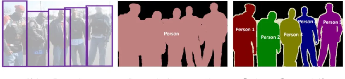
The task of semantic segmentation is of essential importance for a wide range of real world applications. For example, an autonomous car needs to detect the roadsides with a high precision in order to move by itself. In robotics, production machines should be able to delineate the exact shape of an object to perform advanced automatic tasks. Further examples could also include medical image segmentation for automatic disease diagnosis and advanced image editing tools. It is important to note that semantic segmentation does not separate instances of the same class but only focuses on the category of each pixel. In other words, two objects of the same category in the input image will not be distinguished as separate objects. There exists a dierent class of models, known as instance segmentation models, which do distinguish between separate objects of the same class. Figure 2.1 reports an illustration of this dierence.

Figure 2.1: Illustration of dierent computer vision task related to image understanding

The goal of semantic segmentation, in the simplest formulation, is to take either a RGB color image (height×width×3) or a grayscale image (height×

width×1) and output a segmentation map where each pixel contains a class label represented as an integer (height×width×1). More advanced techniques

(14)

4 Chapter 2. Semantic Segmentation

add additional channels to the input image to include 3D information of the environment (depth maps).

Currently, the most performing techniques for semantic segmentation are based on Deep Convolutional Neural Networks. In the following sections these tech-niques will be introduced as well as some state-of-the-art network for semantic segmentation.

2.1 Convolutional Neural Networks

Convolutional neural networks (CNNs) [2] are a specialized kind of neural net-work for processing data that has a known grid-like topology. Some examples include time-series data, which can be thought of as a 1-D grid taking samples at regular time intervals, and image data, which can be considered as a 2-D grid of pixels.

The name "convolutional neural network" indicates that the network employs a mathematical operation called convolution that is a specialized kind of linear operation. Convolutional networks are simply neural networks that use convo-lution in place of general matrix multiplication in at least one of their layers [3]. CNNs are composed of multiple building blocks, some common examples in-cude: convolutional layers, pooling layers, and fully connected layers, that are designed to automatically learn spatial hierarchies of features through a back-propagation algorithm [4].

Convolutional Layer

Convolution is a specialized type of linear operation which in this particular case is used for feature extraction, where a kernel (composed by a 2D array of num-bers), is applied across the input (denoted as input tensor). An element-wise product between each element of the kernel and the input tensor is calculated at each location of the tensor and summed to obtain the output value in the corresponding position of the output tensor, called a feature map. This pro-cedure is repeated applying multiple kernels, with dierent sizes, to form an arbitrary number of feature maps, which represents dierent characteristics of the input tensors. Figure 2.2 shows an illustration of the standard convolution process for 2D data.

(15)

2.1. Convolutional Neural Networks 5

Figure 2.2: Example of standard convolution with a kernel size of 3×3.

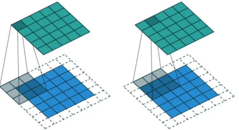
There exists some variations of the standard convolution described above. For example, we may want to skip over some positions of the kernel to reduce the computational cost. This operation is called strided convolution and it can be seen as a downsampling of the output of the full convolution function. It is also possible to dene a separate stride for each direction of motion of the kernel.

Another variation of the standard convolution operation is the dilated convo-lution, also called "Atrous Convolution" [5], that consists in inserting "holes" in the kernel matrix to capture features of the input tensor at a dierent scale. Compared to the increase in the kernel size, this operation does not require ad-ditional computational costs. Figure 2.3 shows an illustation of this technique.

Figure 2.3: Example of atrous convolution with a kernel size of3×3 and dilation factor equal to1.

Finally, the outputs of a linear operation such as convolution are then passed through a nonlinear activation function. There are three functions that are commonly used for this task:

• Sigmoid function: f(x) = 1 1 +e−x

(16)

• Hyperbolic tangent: f(x) = 2

1 +e−2x −1

• Rectied Linear Unit (ReLU): f(x) = max(0, x)

Pooling Layer

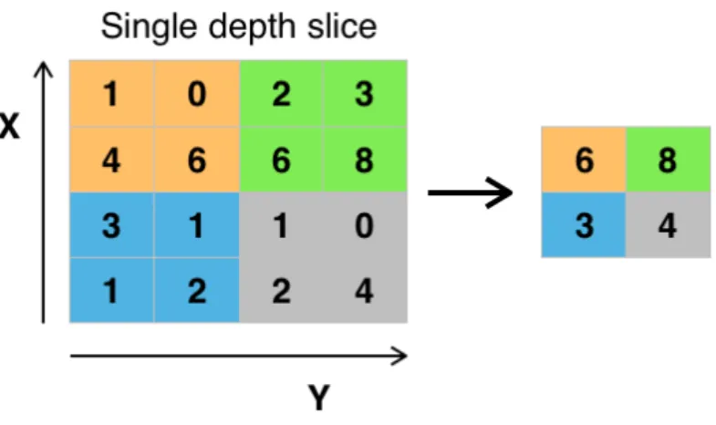
The pooling layer is often used between convolutional layers in a CNN archi-tecture. This layer provides a typical downsampling operation which reduces the in-plane dimensionality of the feature maps in order to introduce a trans-lation invariance to small shifts and distortions, and to decrease the number of subsequent learnable parameters. Typically this layer is used to perform two operations: average pooling and maximum pooling. Maximum pooling extracts patches from the input feature maps, outputs the maximum value in each patch, and discards all the other values. Average pooling instead outputs the average value in each patch. Figure 2.4 shows an illustation of max pooling operation.

Figure 2.4: Example of max pooling operation with a lter size of2×2.

Fully Connected Layer

In the classication problems the output feature maps of the nal convolution or pooling layer is typically attened (i.e. transformed into a one-dimensional vector), and connected to one or more fully connected layers (known as dense layers), in which every input is connected to every output by a learnable weight. In a classication task, the last of these layers typically has the same number of output nodes as the number of considered classes. A common activation function applied to the multi-class classication task is the softmax function which normalizes output real values from the last fully connected layer to target class probabilities, where each value ranges between 0 and 1 and all values sum to 1.

(17)

2.1. Convolutional Neural Networks 7

The softmax function is dened as:

f(x)i =

exi

PK

k=1exk

(2.1)

Where i is the i-th class and K is the number of classes considered for the

classication problem.

This layer was initially used also to perform semantic segmentation, however this had the drawback of limiting the input images to a xed size. For this reason, starting from the idea introduced by the Fully Connected Network (FCN) [6], the dense layers have been substituted by convolutional ones which solve the problem of multiple resolution images and also reduce the computational costs needed to produce the output segmentation maps.

Network Training

Training a network is a process which consists in nding kernels in convolutional layers and weights in fully connected layers which minimize the dierences be-tween output predictions and given ground truth labels on a training dataset. The backpropagation algorithm is the method commonly used for training neu-ral networks where loss function and gradient descent optimization algorithm play essential roles. A loss function, also referred to as a cost function, measures the compatibility between output predictions of the network and given ground truth labels.

Gradient descent is commonly used as an optimization algorithm that iteratively updates the learnable parameters (i.e. kernels and weights) of the network to minimize the loss. The gradient of the loss function provides us the direction in which the function has the steepest rate of increase and each learnable param-eter is updated in the negative direction of the gradient with an arbitrary step size based on a hyperparameter called learning rate. The gradient is, mathemat-ically, a partial derivative of the loss with respect to each learnable parameter, and a single update of a parameter is formulated as follows:

w=w−η· ∂L

∂w (2.2)

Wherew stands for each learnable parameter,η stands for a learning rate, and Lstands for a loss function.

In practice, the learning rate is one of the most important hyperparameters to be set before the training starts. As a consequence of memory limitations,

(18)

the gradients of the loss function with regard to the parameters are computed by using a subset of the training dataset called mini-batch, and applied to the parameter updates. This method is called mini-batch gradient descent, also frequently referred to as stochastic gradient descent (SGD), and the mini-batch size is also a hyperparameter. In addition, many improvements on the gradient descent algorithm have been proposed and widely used, such as SGD with momentum, and Adam [7].

2.2 CNNs for Image Classication

The ImageNet challenge has been traditionally tackled with image analysis al-gorithms such as SIFT with mitigated results until the late 90s. However, a gap in performance has been brought by using neural networks.

The rst deep learning model published by A. Krizhevsky et al. [8] won the 2012 ImageNet competition with a test accuracy of 84.6% outperforming the previous best one with an accuracy of 73.8%. This famous model, the so-called "AlexNet" is what can be considered today as a simple architecture with ve consecutive convolutional lters, max-pool layers and three fully-connected lay-ers.

Simonyan at al. [8] (2014) released the VGG16 model, composed of sixteen convolutional layers, multiple max-pool layers and three nal fully-connected layers. In particular, they chained multiple convolutional layers with ReLU activation functions creating non-linear transformations. Indeed, introducing non-linearities allows models to learn more complex patterns. Moreover they introduced 3x3 lters for each convolution (as opposed to 11x11 lters for the AlexNet model) and noticed they could recognize the same patterns than larger lters while decreasing the number of parameters to train. This model won the 2013 ImageNet competition with 92.7% accuracy.

Szegedy et al. (2014) [9] proposed GoogLeNet (as known as Inception V1), a deeper network with 22 layers using such "inception modules" for a total of over 50 convolutional layers. Each module is composed of 1x1, 3x3, 5x5 con-volutional layers and a 3x3 max-pool layer in order to increase sparsity in the model and obtain dierent type of patterns. The feature maps produced are then concatenated and analyzed by the next inception module. The GoogLeNet model won the 2014 ImageNet competition with accuracy of 93.3%.

(19)

2.3. CNNs for Semantic Segmentation 9

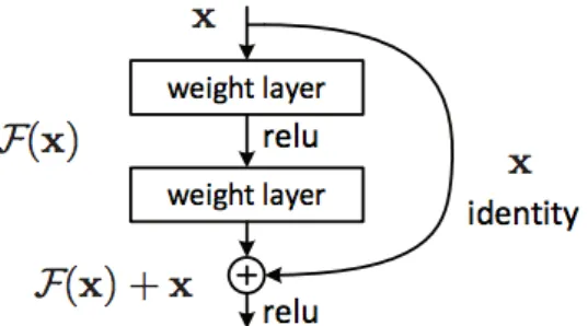
the 2016 ImageNet competition with 96.4% accuracy. It is well-known due to its depth (152 layers) and the introduction of residual blocks. The residual blocks address the problem of training a really deep architecture by introducing iden-tity skip connections between the output of one or multiple convolutional layers and their original input. Consequently, patterns from the input image can be learned in deeper layers. Moreover, this method does not add any additional parameter and does not increase the computational complexity of the model. The residual block is shown in gure 2.5.

Figure 2.5: Basic building block of residual learning framework

2.3 CNNs for Semantic Segmentation

A naive approach towards constructing a neural network architecture for seman-tic segmentation simply consists in stacking a number of convolutional layers (with same padding to preserve dimensions) and output a nal segmentation map. This directly learns a mapping from the input image to its correspond-ing segmentation through the successive transformation of feature mappcorrespond-ings. However this approach is quite computationally expensive and is not used in practice.

It is important to note that for deep convolutional networks, earlier layers tend to learn low-level concepts while later layers develop more high-level (and spe-cialized) feature mappings. A common technique to maintain expressiveness consists in increasing the number of feature maps (channels)as we get deeper in the network.

Currently, the most successful techniques for semantic segmentation are based on the same macro structure that is called Autoencoder. In general, these types of models are composed by two main components: the rst one, which is called Encoder, is a state-of-the-art CNN for classication without its nal fully con-nected layers. The second one, which is called Decoder, is the component that upsamples the feature maps produced by the Encoder to the nal pixel-wise prediction. Decoders are the components that most determine the dierence

(20)

between those models as they dier in the approaches utilized to upsample the resolution of the feature map.

The rst network that adopted such structure was the Fully Convolutional Net-work (FCN) by Long et al. [6]. They transformed the existing and well-known classication models into fully convolutional ones by replacing the fully con-nected layers with convolutional ones to output spatial maps instead of classi-cation scores. Those maps are upsampled using fractionally strided convolutions to produce dense per-pixel labeled outputs. This work is considered a milestone since it showed how CNNs can be trained end-to-end for this problem, eciently learning how to make dense predictions for semantic segmentation with inputs of arbitrary sizes [11].

Badrinarayanan et al.[12] presented SegNet, a variant of FCN in which the decoder stage is composed by a set of upsampling and convolutional layers which are at last followed by a softmax classier to predict pixel-wise labels. Each upsampling layer in the decoder corresponds to a max-pooling one in the encoder-part. This operation is performed using the max-pooling indices from the corresponding feature maps in the encoder phase. The upsampled maps are then convolved with a set of trainable lters to obtain dense features maps. Ronneberger et al.[13] introduced the U-Net architecture which is an improve-ment of FCN. They modied the fully convolutional architecture by expanding the capacity of the decoder module. The architecture consists in a contracting path to capture context and a symmetric expanding path that enables precise localization.

Lin et al. [14] introduced the Feature Pyramid Network (FPN) an architecture that shows signicant improvement as a generic feature extractor in several applications. In particular, they exploited the inherent multi-scale, pyramidal hierarchy of deep convolutional networks to construct feature pyramids with a marginal extra cost. A top-down architecture with lateral connections is devel-oped for building high-level semantic feature maps at all scales.

Zhao et al.[15] proposed the Pyramid Scene Parsing Network (PSPNet) to bet-ter learn the global context representation of a scene. Patbet-terns are extracted from the input image using a feature extractor like ResNet [10] with a dilated network strategy. Then the feature maps are fed to a Pyramid Pooling Mod-ule to distinguish patterns with dierent scales. Features are pooled with four dierent scales each one corresponding to a pyramid level and processed by a 1x1 convolutional layer to reduce their dimensions. With this technique each

(21)

2.3. CNNs for Semantic Segmentation 11

pyramid level analyses sub-regions of the image with dierent location. The outputs of the pyramid levels are upsampled and concatenated to the inital fea-ture maps to contain the local and the global context information. Finally, they are processed by a convolutional layer to generate the pixel-wise predictions. Chen et al. [16] presented the Deeplab v2, an autoencoder network based on ResNet network [10]. In particular, they removed the down-sampling operator from the last few max pooling layers of DCNNs and instead upsampled the lters in subsequent convolutional layers. Filter upsampling consists in inserting holes between nonzero lter taps. In [16] they used the term atrous convolution as a shorthand for convolution with upsampled lters. Moreover to handle objects at multiple scales, they employed multiple parallel atrous convolutional layers with dierent sampling rates and they called the proposed technique "Atrous Spatial Pyramid Pooling" (ASPP). Finally, they boosted the model's ability to capture ne details by employing a fully connected Conditional Random Field (CRF) [17].

(22)

(23)

13

3 Unsupervised Techniques for

Semantic Segmentation

As mentioned in the initial problem statement, the goal of this work is to develop and test new techniques which improve the accuracy of semantic segmentation models in all the situations in which large datasets are not available or very costly to produce.

The way to achieve this is to nd the best method to extract useful information from unlabeled data that can be used to reinforce the standard supervised training. We chose to utilize a framework based on GANs [18] that is very commonly used for this task.

The work for this thesis is based on the work of Hung et al. [1] that proposed a new technique to reinforce the adversarial training with unsupervised data. This and other techniques will be discussed in details in the following sections.

3.1 Generative Adversarial Networks

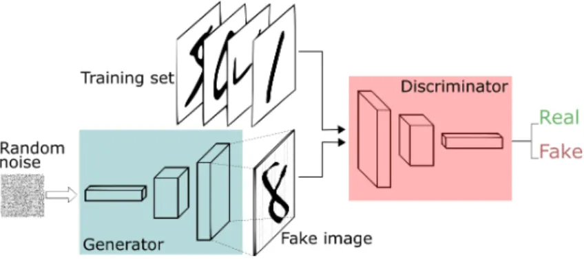
Goodfellow et al. [18] in 2015 proposed a new framework for estimating gen-erative models via an adversarial network. This framework, called Gengen-erative Adversarial Networks (GANs), is composed by two networks pitted against each other: a generative model G (Generator) that captures the data distribution,

and a discriminative model D (Discriminator) that estimates the probability

that a sample came from the training data rather than from G. Figure 3.1

illustrates an example of a basic GAN structure.

As described in the paper [18], the network G takes samples z from a xed

distribution Pz(z), and transforms them to approximate the distribution of training samplesx. The adversarial networkD is used to dene a loss function

which is used to explicitly evaluate the output produced byG. This framework

corresponds to a min-max two-player game with the following value function:

V(G, D) : min

(24)

14 Chapter 3. Unsupervised Techniques for Semantic Segmentation

Figure 3.1: Example of a GAN Structure.

In the space of arbitrary functions G and D, a unique solution exists, with G

recovering the training data distribution andD equal to 1/2everywhere. The adversarial model is trained to optimally discriminate samples from the empirical data distribution and samples from the deep generative model. The generative model is concurrently trained to minimize the accuracy of the ad-versarial, which provably drives the generative model to approximate the dis-tribution of the training data. The adversarial network can be interpreted as a "variational" loss function, in the sense that the loss function of the generative model is dened by auxiliary parameters that are not part of the generative model.

As originally explained by the authors, GANs can be thought of as analogous to a team of counterfeiters, trying to produce fake currency and use it without detection, while the discriminative model is analogous to the police, trying to detect the counterfeit currency. Competition in this game drives both teams to improve their methods until the counterfeits are indistinguishable from the genuine articles [18].

The original GAN was developed using Multi-Layer Perceptrons, but later ver-sions using deep convolutional GANs (DCGAN [19]) instead have shown im-pressive improvements in the task of generating realistic data.

As originally suggested by the authors, adversarial networks can be used to perform semi-supervised learning: features captured by the discriminator can be used to improve the performance of classiers when limited labeled data is available. The work of this thesis is based on this idea applied to semantic image segmentation.

(25)

3.2. Adversarial Networks Applied to Semantic Segmentation 15

3.2 Adversarial Networks Applied to Semantic

Segmentation

The adversarial networks, as dened in the section above, were used in the original paper to discriminate between the data produced by the generator and the sample from the real distribution. To apply this framework to the eld of semantic segmentation we need to take in account the dierence between the two problems.

As discussed in Chapter 2, semantic segmentation models aim to map an input image into the corresponding segmentation map. This can be done by training the network in a supervised manner using the labels provided with the input data.

Using the same terminology of the GANs framework we can identify the seg-mentation network as the generator that "generates" segseg-mentation maps corre-sponding to the input images. The adversarial network (discriminator) in this case has the task of discriminate between the segmentation maps produced by the generator and the ground truth labels associated to the input images. Luc et al. [20] in 2016 proposed this approach for semantic segmentation. They utilized a FCN as the generator network and a CNN as the discriminator net-work. In their setup the generator network is trained with a combination of two loss functions: the classical cross-entropy loss between input data and corre-sponding labels and the adversarial loss provided by the discriminator. As dis-cussed by the authors of [20], the adversarial loss encourages the segmentation model to produce label maps that cannot be distinguished from ground-truth ones by an adversary binary classication model.

(26)

3.3 Semi-Supervised Semantic Segmentation

Tech-niques

Semantic segmentation architectures are typically trained on huge datasets with pixel-wise annotations (e.g., the Cityscapes [21] or CamVid [22] datasets), which are highly expensive, time-consuming and error-prone to generate. To overcome this issue, semi-supervised methods are emerging, trying to exploit weakly an-notated data (e.g., with only image labels or only bounding boxes) [23, 24, 25, 26, 27, 28, 29] or completely unlabeled [30, 31] data after a rst stage of super-vised training.

In 2015 Papandreou et al. [32] introduced a novel Expectation-Maximization (EM) methods for training DCNN semantic segmentation models from weakly annotated data. The proposed algorithms alternate between estimating the la-tent pixel labels (subject to the weak annotation constraints), and optimizing the DCNN parameters using stochastic gradient descent (SGD). Additionally they show how the EM approach also excels in the semi-supervised scenario. In particular, they show that having access to a small number of strongly (pixel-level) annotated images and a large number of weakly (bounding box or image-level) annotated images, the proposed algorithm can almost match the perfor-mance of the fully-supervised system.

In 2017 Souly et al. [33] proposed a weakly supervised semantic segmenta-tion framework using GANs. In their work they extended GANs by replacing the traditional discriminator D with a fully convolutional multi-class classier, which, instead of predicting whether a sample x belongs to the data distribu-tion, assigned to each input image pixel a labely from the K semantic classes

or mark it as fake sample assigning the classK+ 1. To train this network they fed three inputs to the discriminator: labeled data, unlabeled data and fake data.

Hung et al. [1] developed a dierent framework for semi-supervised semantic segmentation. Dierently from other competing approaches they did not uti-lize weakly annotated images to improve the accuracy, instead they proposed a framework based on GANs that uses unlabeled data to boost the standard training process. In contrast to the typical GANs discriminators, which take xed sized input images and output a single probability value, they employed a fully-convolutional network that can take inputs of arbitrary sizes. After obtaining the initial segmentation prediction of the unlabeled image from the

(27)

3.4. Domain Adaptation Techniques 17

segmentation network, they computed a condence map by passing the segmen-tation prediction through the discriminator network. This condence map is then used as a supervisory signal for a self-taught scheme to train the segmen-tation network with a masked cross-entropy loss.

We based the work of this thesis on the work proposed in [1] since it has demon-strated good performances on some commonly used datasets for semantic seg-mentation.

3.4 Domain Adaptation Techniques

In addition to the aforementioned approaches to tackle the lack of data, an increasingly popular alternative is represented by domain adaptation from syn-thetic data. The development of sophisticated computer graphics techniques enabled the production of huge synthetic datasets for semantic segmentation purposes at a very low cost. To this end, several synthetic datasets have been built, e.g., GTA5 [34] and SYNTHIA [35] which have been employed in this work. The real challenge is then to address the cross-domain shift when a neu-ral network trained on synthetic data needs to process real-world images since in this case training and test data are not drawn i.i.d. from the same underlying distribution as usually assumed [36, 37, 38, 39].

A possible solution is to process synthetic images in order to reduce the inher-ent discrepancy between source and target domain distributions mainly using generative networks (i.e., GANs) [40, 41, 42, 43, 44]

Unsupervised domain adaptation has been already widely investigated in clas-sication tasks [45, 46, 47]. On the other hand, its application to semantic segmentation is still a quite new research eld.

The rst work to investigate cross-domain urban scene semantic segmentation is [48], where an adversarial training is employed to align the features from the dierent domains. In particular, they introduced a pixel-level adversarial loss to the intermediate layers of the network and imposed constraints to the network output.

In 2017 Zhang et al. [49] presented a curriculum-style learning approach to solve the problem of domain adaptation. In particular, they rstly learn to estimate the global label distributions of the images and local label distributions of the landmark superpixels of the target domain. Then they used these results to eectively regularize the training of the semantic segmentation network forcing

(28)

its predictions to meet the inferred label distributions over the target domain. Following these approaches, many works addressed the source to target domain shift problem with various techniques [50, 51, 52, 53, 53, 54].

As an example, Sankaranarayanan et al. [55] in 2017, proposed an approach based on GANs to reduce the domain shift between two domains. In particular, they proposed a joint adversarial approach that transfers the information of the target distribution to the learned embedding using a generator-discriminator pair.

Homan et al. [56] in 2018 presented a cycle-consistent adversarial domain adaptation method that unies cycle-consistent adversarial models with adver-sarial adaptation methods. The proposed framework is able to adapt even in the absence of target labels and is broadly applicable at both the pixel-level and in feature space.

(29)

19

4 Proposed Methods

The work of this thesis is based on the work proposed in [1], which has been introduced in Chapter 3.

We utilized this framework as a baseline for our tests and we developed some extensions that further improve the performances of the unsupervised training process.

Firstly, we considered a scenario in which a limited amount of annotated data are available for a specic problem. We used this framework to train the net-work gathering information from both labeled and unlabeled images. This has a lot of advantages since unlabeled data can be gathered without any eort compared to the annotated ones, thus we can exploit huge unlabeled datasets to boost the segmentation network training.

As introduced in [18], this technique follows the idea of using the features learned by the discriminator network to improve the performances of the generator even with unlabeled data.

Dierently from the previous problem, for domain adaptation we used this framework with data coming from two dierent datasets. In particular, we used a computer generated dataset to perform supervised training and a real world scenes dataset as our unsupervised input.

We investigated a scenario where a large amount of annotated synthetic data is available but there is no labeled real world data available.

Using this framework we tried to take advantage of unsupervised loss provided by the discriminator to reduce the domain shift between synthetic and real data.

(30)

20 Chapter 4. Proposed Methods

4.1 Network Structure

In this section the overall system architecture will be introduced.

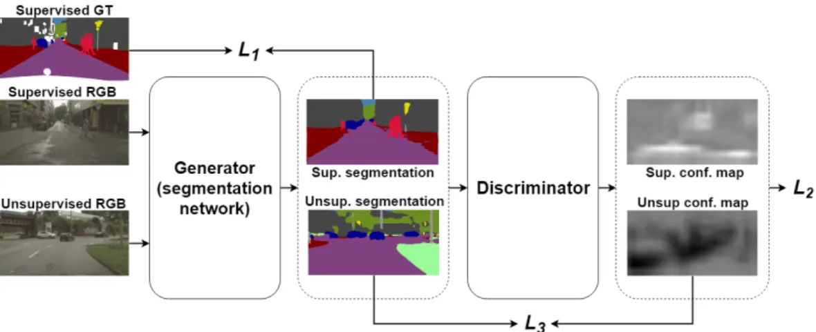
The general architecture of the proposed network is shown in Figure 4.1. This network is based on the framework proposed in [1]. The network is composed by two main blocks: the segmentation network and the discriminator network.

Figure 4.1: The architecture of the proposed framework for semi-supervised semantic segmentation. A rst stage of supervised learning with annotated data is followed by a second stage of unlabeled data to boost the performance of the segmentation network through the combination of 3 losses. L₁ is a standard

cross-entropy loss between the generated synthetic segmentation maps and their respective ground truth. L2 is an adversarial loss based on the condence map

generated by a fully-convolutional discriminator network, which is trained with a spatial cross-entropy loss (L_D). L₃ is a novel loss for unlabeled data.

The segmentation network is a Deeplab v2 [16] which, as described in Chap-ter 2, is an autoencoder network based on ResNet [10] CNN. We considered to use Deeplab v2 since it has very good performances, however this approach does not rely on specic properties of this network and it can be substituted with any network for semantic segmentation. Furthermore in this work we have not employed the CRF since it is a post-processing technique that is used only for the output segmentation map.

The discriminator network in the problem of semantic segmentation aims at dis-criminating images produced by the segmentation network (fake images) from the corresponding ground truth images (real images).

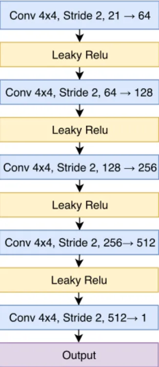
The network used for the experiments is a fully convolutional network composed by 5 convolutional layers each followed by a leaky Rectied Linear Unit (ReLU) activation function.

(31)

4.1. Network Structure 21

small gradient signal for negative values. As a result, it makes the gradients from the discriminator ow stronger into the generator.

Dierently from other adversarial learning models, this network produces a per-pixel prediction instead of a single binary value for the whole input image. The parameters of the discriminator network are reported in Figure 4.2.

Conv 4x4, Stride 2, 21 → 64 Leaky Relu Conv 4x4, Stride 2, 64 → 128 Leaky Relu Conv 4x4, Stride 2, 128 → 256 Leaky Relu Conv 4x4, Stride 2, 256→ 512 Leaky Relu Conv 4x4, Stride 2, 512→ 1 Output

Figure 4.2: Discriminator network used for the experiments. For each block are reported: block type, kernel size, stride dimension, channels. The dimension of the output of the last block is referred to the training on the PASCAL VOC2012 dataset

(32)

4.2 Network Training Strategies

In this section we explain in details the techniques utilized to train the frame-work described above.

The main idea is to use a composed loss function to optimize the generator network with the standard back-propagation algorithms. This function is com-posed by dierent terms that exploit informations coming from both labeled and unlabeled data.

Given an input image Xn of size H×W ×3 and its one-hot encoded ground truthYn, we denote the segmentation network byG(·)and the predicted prob-ability map by G(Xn) of size H ×W ×C where C is the classes number. We denote the fully convolutional discriminator byD(·) which takes a probability map of size H ×W ×C and outputs a condence map of size H ×W ×1. Finally to distinguish between data coming from the supervised dataset and the unsupervised one we use the terms Xs_n and Xu_n respectively.

The loss of the discriminator LD is a standard cross-entropy loss between the produced map and the one-hot encoding related to the fake domain (class 0) or ground truth domain (class 1) depending on the fact that the input has been respectively drawn from the generator or from ground truth. This loss term is dened by:

LD =−

X

h,w

log(1−D(G(Xs,u_n ))(h,w)) + log(D(Y_ns)(h,w)) (4.1) Where D(G(Xn))(h,w)) is the condence map of Xn at location (h,w), and

D(Ys

n)(h,w) is the condence map ofYsn at location (h,w) .

Notice that the discriminator has to label with 0 the segmentation maps pro-duced by the generator using both annotated data from the supervised dataset (denoted withX_ns) and unlabeled data from the unsupervised dataset (i.e., X_nu).

The loss term indicated asL1 is the standard cross-entropy function utilized to train the network only with annotated data and is dened by:

L1 =− X h,w X c∈C (Y_ns)(h,w,c)log(G(Xs_n)(h,w,c)) (4.2) The loss term indicated asL2 is the adversarial loss driven by the discriminator network and is dened by:

Ls,u₂ =−X

h,w

(33)

4.2. Network Training Strategies 23

This term force the training of the generator network in the direction of fooling the discriminator producing data that resembles the ground truth statistics. Moreover it can be applied even with unlabeled data since it requires only the output of the segmentation network to be evaluated.

Finally the loss term L3 introduced in [1] is dened by the authors as a self-taught learning framework. The main idea is that the trained discriminator can generate a condence map D(G(Xu_n)) which can be used to infer the regions suciently close to those from the ground truth distribution. The self-taught, one-hot encoded ground-truth_Yˆ _{is an element-set with} _Yˆ(h,w,c∗₎

n = 1 if

c∗ = argmax_c(G(Xn)(h,w,c)). The resulting semi-supervised loss is dened by:

L3 =− X h,w X c∈C I(D(G(Xu_n))(h,w) > Tsemi)·Yˆ(nh,w,c)log(G(X u n) (h,w,c)₎ _(4.4)

where I(·) is the indicator function and Tsemi is the threshold to control the sensitivity of the self-taught process.

Since _Yˆ

n and I(·) are used as constant during training, Equation (4.4) can be simply viewed as a masked spatial cross entropy loss.

To conclude, a weighted average of the three losses is used to train the generator exploiting the proposed adversarial learning framework, i.e.,:

LG =L1+λsadv· L s 2+λ u adv· L u 2 +λsemi· L3 (4.5)

where λs_adv, λu_adv and λsemi are three parameters that controls the inuence of each related loss.

The discriminator is fed both with ground truth labels and with the generator output computed on a mixed batch containing both labeled and unlabeled data and is trained aiming at minimizing LD. Concerning the generator, instead, during the rst 5000 steps L3 is disabled (i.e. λsemi is set to 0) thus allowing the discriminator to enhance its capabilities to produce higher quality condence maps before using them.

Proposed loss variants

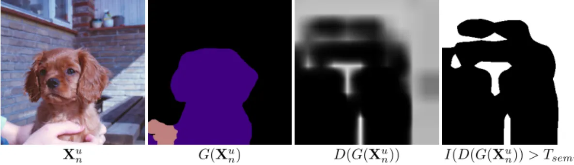
As we can observe in Figure 4.3 the semi-supervised framework described above produces a condence map that has high condence (represented in white in the third image of Figure 4.3) in the center of the biggest segmented areas and very low condence (represented in black in the third image of Figure 4.3) in the area

(34)

corresponding to a change of class (i.e. edges/boundaries) in the segmentation map.

Xun G(Xun) D(G(Xun)) I(D(G(Xun))> Tsemi)

Figure 4.3: Overview of discriminator output during the training phase.

We designed a modied semi-supervised loss to tackle this problem with the goal of gathering more information from the generated condence map. We indicate as De(·) the normalized version of D(·) dened by the following linear

function:

e

D(G(Xn))(h,w) =

D(G(Xn))(h,w)−Dmin(G(Xn))

Dmax(G(Xn))−Dmin(G(Xn)) (4.6) Where Dmax(·) and Dmin(·) indicate the maximum and the minimum values assumed byD(·) respectively.

Instead of selecting only the most condent regions of D(·), we used the full output of the discriminator as a weighting function for the cross-entropy loss evaluation. In particular we give large relevance to the regions that look like ground truth and then smaller and smaller up to no relevance to region marked as fake by the discriminator.

The designed semi-supervised loss indicated as L3,1 is dened by the following function: L3,1 =− X h,w X c∈C e D(G(Xu_n))(h,w)·Yˆ_n(h,w,c)log(G(Xu_n)(h,w,c)) (4.7) This loss can be seen as smoothed self cross-entropy considering thatDe(G(X_n))

acts as a weighting function for the term_Ynˆ _{described in Equation (4.4). Notice} that, as in Equation (4.4), only the term Xu_n corresponding to unlabeled data is used for the evaluation of this loss.

Considering the task of domain adaptation, the unsupervised loss termsL3 and

L3,1 forces the generator to adapt to the target domain, thus producing maps that resemble the ground truth ones as in the scenario of a single dataset. As we can observe in Figure 4.4, unlabeled data would lead the model to pro-duce a less noisy result in the areas corresponding to large classes in the input

(35)

4.2. Network Training Strategies 25

images. However, at the same time, this loss contribution leads the model to mislead rare and tiny objects (such as trac lights, pole or person).

In particular we can observe that the contribution of the designed loss L3,1 in this case produces worse visual results compared to Hung et al. (L3).

Image Annotation Baseline (L1) Hung et al. [1] Ours (L3,1)

Figure 4.4: Overview of proposed technique applied to domain adaptation

To overcome this behavior we designed another variation of theL3 loss. The new loss term indicated byL3,2 is dened by:

L3,2 =− X h,w X c∈C I(D(G(X_nu))(h,w) > Tsemi)·Wcs·Yˆ (h,w,c) n log(G(X u n) (h,w,c) )) (4.8) Where W_cs is a weighting function computed on the source domain dened as:

W_cs= 1− P n|p∈Xn∧p∈c| P n|p∈Xn| (4.9)

Where we indicated as p a pixel of image Xn and |·| represents the cardinality of the considered set.

This corrective term serves as a balancing factor when unlabeled data of the target set are used. Notice that the term comes into play only when using unla-beled data of the target domain but the class frequencies have to be computed on the labeled data of the source domain since we need the ground truth labels to evaluate it. This calculation has only to be performed a priori and it is not changed as the learning progresses.

The results of the dierent modied losses compared to [1] are reported in Chapter 5.

(36)

(37)

27

5 Results

5.1 Experimental Setup

The original framework on which this thesis is based [1] was developed using Pytorch1 _{version 0.2. We chose to re implement this framework using} Tensor-ow2 _{version 1.12.0 because it is more supported than Pytorch and includes} some tools like Tensorboard, which is a powerful suite that allows debug and visualization of the learning process.

To perform the trainings we utilized a single Nvidia 1080Ti GPU, which has 12GB of dedicated memory. The limited amount of available resources forced us to reduce the batch size and the images resolution until the networks tted in memory. Moreover with this conguration the longest training we performed took about 20 hours to complete.

All the experiments were performed using the same parameters to train the network. We chose these parameters after some preliminary tuning of the pro-posed architecture. In particular we trained the generator network (G) using the

standard technique proposed by [16] with Stochastic Gradient Descent (SGD) as optimizer with momentum set to 0.9 and weight decay to 10−4. The dis-criminator network (D) has been trained using the Adam optimizer [7]. The

learning rate employed for bothGand D started from10−4 and was decreased up to10−6 by means of a polynomial decay with power0.9.

We set the weighting parameters empirically to balance between the three com-ponents as: λs_adv = 10−2 for annotated data, λu_adv = 10−3 to give less weight in case of unlabeled data andλsemi = 10−1. Finally we setTsemi = 0.2to obtain a signicant mask from the condence map.

For the generator network we used the standard Deeplab v23 _{without CRF [17]} and based on the ResNet-101 model whose weights were pre-trained on the MSCOCO dataset [57]4_.

1_{https://pytorch.org/}

2_{https://www.tensorflow.org/}

3_{We used the network provided by Wang and Ji available at}

https://github.com/zhengyang-wang/Deeplab-v2--ResNet-101--Tensorflow/ 4_{We used the weights computed by V. Nekrasov available at}

(38)

28 Chapter 5. Results

Tensorow

TensorFlow is an open source software library for high performance numerical computation. Its exible architecture allows easy deployment of computation across a variety of platforms (CPUs, GPUs, TPUs), and from desktops to clus-ters of servers to mobile and edge devices. Originally developed by researchers and engineers from the Google Brain team within Google's AI organization, it comes with strong support for machine learning and deep learning and the ex-ible numerical computation core is used across many other scientic domains.

5.2 Datasets

In this section we introduce the datasets that we used to evaluate the perfor-mances of the semi-supervised framework and the proposed method for unsu-pervised domain adaptation.

To test the eectiveness of the proposed semi-supervised framework we used two publicly available datasets, namely PASCAL VOC2012 [58] and Cityscapes [21].

For the domain adaptation task we want to show that it is possible to train a semantic segmentation network in a supervised way on synthetic datasets and then apply unsupervised domain adaptation to real data in autonomous driv-ing scenarios. Thus, we used two synthetic datasets, namely GTA5 [34] and SYNTHIA [35] for the supervised part of the training, while the unsupervised adaptation and the result evaluation have been performed on the real world Cityscapes [21] dataset.

PASCAL VOC2012 [58] is composed by 10,582 color images with dier-ent resolutions, represdier-enting a large number of visual object in realistic scenes. They have a pixel level semantic annotation with 21 classes. Since the labels for the original test set are not available, we rearranged the original training and validation sets for our experiments. Accordingly to what has been done in [1], we used the original validation set, composed by1449annotated images, as our validation and test dataset.

Before feeding the images to the network we performed data augmentation ap-plying a random scale between 0.5 and 1.5 and then a random crop of size 321×321 to have images of the same dimension.

CITYSCAPES [21] is composed by 2,975 high resolution color images captured on the streets of 50dierent European cities. They have a pixel level semantic annotation with34classes of which only19are taken in consideration

(39)

5.2. Datasets 29

Figure 5.1: Examples of images of the PASCAL VOC2012 dataset

for training and testing. Since the labels for the original test set are not avail-able, we rearranged the original training and validation sets for our experiments. We randomly divided the original training split in a training set, composed by 2,475 images, and a validation set, composed by500 images. The original high resolution images have been resized to375×750 pixel for memory constraints. The testing was instead carried out on the original resolution of 2048×1024 pixel.

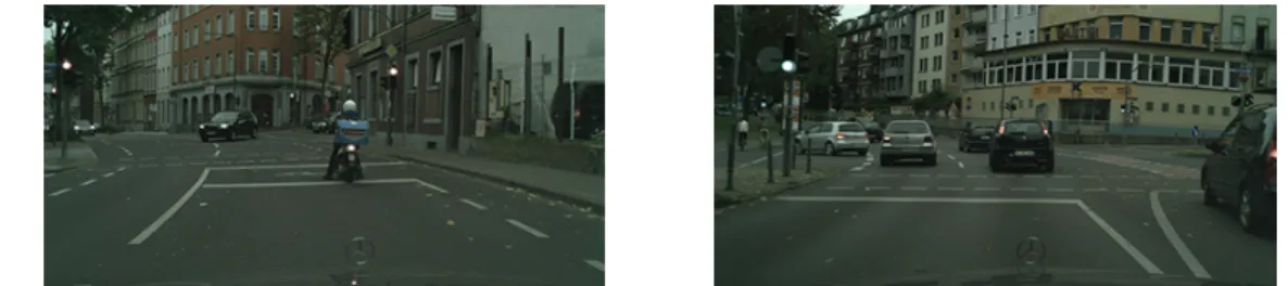
Figure 5.2: Examples of images of the Cityscapes dataset

GTA5 [34] is a huge dataset composed by 24966 photo-realistic synthetic images with pixel level semantic annotation. The images have been recorded from the prospective of a car in the streets of virtual cities (resembling the ones in California) in the open-world video game Grand Theft Auto 5. Being taken from a high budget commercial production they have an impressive visual quality and are very realistic. In our experiments, we used 23966 images for the supervised training and1000 images for validation purposes. There are 19 semantic classes which are compatible with the ones of the Cityscapes dataset. The original resolution of the images is 1914×1052 pixel but we rescaled and cropped them to the size of375×750 pixelfor memory constraints before being fed to the architecture.

SYNTHIA [35] is a very large dataset of photo-realistic images. It has been produced with an ad-hoc rendering engine, allowing to obtain a large variability of the images. On the other hand, the visual quality is not the same of the commercial video game GTA5. We used the SYNTHIA-RAND-CITYSCAPES

(40)

Figure 5.3: Examples of images of GTA5 dataset

version of the dataset, which contains9400images with annotations compatible with16of the19classes of Cityscapes. These images have been captured on the streets of a virtual European-style town in dierent environments under various light and weather conditions. As done in previous approaches, we randomly extracted 100 images for validation purposes from the original training set, while the remaining part, composed by9300 images, is used for the supervised training of our networks. Again, the images have been rescaled and cropped from the original size of760×1280 pixelto375×750 pixel. For the evaluation of the proposed unsupervised domain adaptation on the Cityscapes dataset, only the 16classes contained in both datasets are taken into consideration.

Figure 5.4: Examples of images of SYNTHIA dataset

5.3 Semi-Supervised Semantic Segmentation

In this section we present the results obtained from each of the techniques de-scribed in Chapter 4.

The rst goal of this work was to demonstrate the eectiveness of the chosen semi-supervised framework. To test this we utilized two real-world datasets: PASCAL VOC2012 and Cityscapes. For each dataset we followed the same training strategy: we utilized half of the training set with annotations to com-pute the supervised loss terms and the remaining data as unsupervised input to perform the unsupervised learning.

To test the eectiveness of the proposed approach, for each considered dataset, we performed 4 dierent tests in which we use dierent combinations of loss term to optimize the network:

(41)

5.3. Semi-Supervised Semantic Segmentation 31

• supervised baseline: L1 (indicated as Baseline)

• supervised adversarial: L1+λsadv · Ls2 (indicated as Adversarial)

• semi-supervised framework: L1 +λsadv · Ls2 +λuadv · Lu2 +L3 (indicated as Hung et al. [1])

• proposed method: L1+λsadv · Ls2+λuadv · Lu2 +L3,1 (indicated as Ours)

Results on the PASCAL VOC2012 Dataset

With this dataset we trained the network for 40000 steps with a batch com-posed by 3 images, which was the maximum number allowed by the memory constraints.

Table 5.1 shows two evaluation metrics: the mean Intersection over Union (IoU) and mean pixel accuracy evaluated on the dierent tested techniques. Table 5.2 shows the mean intersection over union evaluated for each single class of the dataset.

As we can see from Table 5.1, the original semi-supervised framework presented by [1] improves mean IoU score by0.5%and mean pixel accuracy score by0.13%, compared to the fully supervised adversarial training technique. Furthermore the proposed variation of the semi-supervised framework brings a further im-provement in both the evaluation metrics. In particular from Table 5.2 we can see how the proposed technique improves the results in some of the considered classes.

Mean IoU Mean Pixel Accuracy

Baseline 72.38 93.71

Adversarial 73.51 93.97

Hung et al. [1] 74.02 94.10

Ours (L3,1) 74.38 94.17

Table 5.1: Mean results of dierent techniques evaluated on the original PASCAL VOC2012 validation dataset.

(42)

bac

kground

aeroplane bicycle bird boat bottle bus car cat chair cow dining

table

dog horse motorbik

e

person potted

plan

t

sheep sofa train tv/monitor Baseline 93.2 87.2 37.4 84.9 64.6 75.5 92.2 84.4 88.6 32.8 75.5 53.6 81.9 77.9 78.2 83.3 52.4 77.8 43.6 83.9 71.1 Adversarial 93.7 86.3 38.9 85.2 66.9 78.7 93.2 85.5 88.0 35.8 75.9 58.8 80.3 77.5 80.5 83.0 54.1 80.9 44.2 83.8 72.8 Hung et al. [1] 93.7 86.6 38.5 86.7 69.7 76.5 93.1 85.2 88.8 33.2 80.1 60.0 81.8 80.6 78.8 83.1 55.3 81.5 44.5 85.9 71.0 Ours (L3,1) 93.8 86.6 38.8 86.3 67.7 76.9 92.6 83.9 88.7 35.0 81.0 62.9 81.7 82.1 79.6 83.2 55.6 82.4 46.3 83.2 73.7

Table 5.2: Mean intersection over union on the dierent classes of PASCAL VOC2012 evaluated on the original validation dataset.

Figures 5.5 and 5.6 reports the plot of the training error of G and D

re-spectively during the training process. Figures 5.7 and 5.8 reports the plot of the mean IoU and mean pixel accuracy evaluated on the validation set. Finally Figure 5.9 reports the plot of the validation error on the PASCAL VOC2012 validation set.

We evaluated the metrics on the validation error every1000 steps to reduce the time needed for the training.

As we can see in Figure 5.9, when we include the discriminator network in the training process the validation error tends to increase over time.

On the contrary the mean IoU metric and the pixel accuracy continue to im-prove. In a standard scenario the raise of the validation error suggests that the network is overtting on the training data, however this is not the case since the other evaluation metrics, specic for semantic segmentation, are improving during the training process. This is a common behavior that has been observed when using adversarial networks: generator and discriminator are competing against each other, hence improvement on the one means a higher loss on the other. However the increment of the generator error (after that the discrimi-nator starts to learn) does not aect the quality of the output images, which instead seems to be improved by the contribution brought by the discriminator. This increase in the network accuracy can be achieved only with an accurate tuning of the training parameters, i.e. learning rate or the various weighting terms. First of all it is essential to tune the learning rate of the generator and discriminator in a way that allows both to improve simultaneously. Moreover a too high value for the weighting terms λs,u_adv and λsemi can lead the generator error to diverge rapidly by the inuence of the discriminator.

(43)

5.3. Semi-Supervised Semantic Segmentation 33 0 0,2 0,4 0,6 0,8 1 1,2 1,4 1,6 1,8 2 0 5000 10000 15000 20000 25000 30000 35000 40000 Gener at or tr ai nin g err or Training step Baseline Adversarial Hung et al. Ours

Figure 5.5: Generator training error on the PASCAL VOC2012 dataset. The error is computed on the batch fed to the network at the corresponding step.

0,25 0,3 0,35 0,4 0,45 0,5 0,55 0,6 0,65 0,7 0 5000 10000 15000 20000 25000 30000 35000 40000 Discrimina tor tr ai nin g err or Training step Adversarial Hung et al. Ours

Figure 5.6: Discriminator error on the PASCAL VOC2012 training dataset. The error is computed on the batch fed to the network at the corresponding step.

(44)

34 Chapter 5. Results 0,6 0,62 0,64 0,66 0,68 0,7 0,72 0,74 0,76 0 5000 10000 15000 20000 25000 30000 35000 40000 Mean Io U Training step Baseline Adversarial Hung et al. Ours

Figure 5.7: Mean IoU on the PASCAL VOC2012 validation dataset evaluated in the training phase.

0,9 0,905 0,91 0,915 0,92 0,925 0,93 0,935 0,94 0,945 0 5000 10000 15000 20000 25000 30000 35000 40000 Mean pix el accur acy Training step Baseline Adversarial Hung et al. Ours

Figure 5.8: Mean Pixel Accuracy on the PASCAL VOC2012 validation dataset evaluated in the training phase.

(45)

5.3. Semi-Supervised Semantic Segmentation 35 0 0,1 0,2 0,3 0,4 0,5 0,6 0 5000 10000 15000 20000 25000 30000 35000 40000 V al ida tion err or Training step Baseline Adversarial Hung et al. Ours

Figure 5.9: Validation error on the PASCAL VOC2012 validation dataset evaluated in the training phase.

In Figure 5.10 are reported some examples of output segmentation maps produced after the training of the network. As we can see from the images, the visual results conrm what emerges from the evaluation metrics: the network trained with the proposed method produces better segmentation maps com-pared to the other techniques. In particular we can observe how the proposed method enhances the boundaries of the segmentation map in correspondence of a class change and it helps to reduce the overall noise of the image.

As we can see in Figure 5.11 there are also some cases in which the proposed method has worse results compared to the other versions. If we focus on the examples in the last row, we can clearly see that the proposed method has some issues in predicting the chair's class. This particular case is a challenging one because it can have an ambiguous interpretation, indeed the object represented in the image is shaped like a chair but has some features that are commonly present on a sofa.

Additional output segmentation maps produced on the PASCAL VOC2012 val-idation set can be found in Appendix A.

(46)

Backgound Aeroplane Bicycle Bird Boat Bottle Bus Car Cat Chair Cow Dining-Table Dog Horse Motorbike Person Potted_Plant Sheep Sofa Train TV/Monitor

Image Annotation Baseline Adversarial Hung et al. [1] Ours (L3,1)

Figure 5.10: Examples of correct semantic segmentation of some sample scenes extracted from the PASCAL VOC2012 validation dataset. The network is trained using half of the dataset as annotated data and the remaining as unsupervised data

Figure 5.11: Examples of incorrect semantic segmentation of some sample scenes extracted from the PASCAL VOC2012 validation dataset. The network is trained using half of the dataset as annotated data and the remaining as unsupervised data

(47)

Results on the Cityscapes Dataset

With this dataset we trained the network for40000steps with a batch composed of only one image to t the memory constraints.

For this dataset we performed the same tests that were performed for the PAS-CAL VOC2012 dataset to have a fair comparison.

As in the previous dataset we reported the two evaluation metrics and the mean IoU computed for each dierent class of the dataset.

As we can see from the results (Tables 5.3 and 5.4), even using this dataset the proposed method has higher scores in both the evaluation metrics. The semi-supervised technique of Hung et al. [1] instead has a lower mean IoU compared to the supervised adversarial training.

If we observe Table 5.2 we can see how the proposed technique improves the results in the majority of the considered classes.

These results are quite dierent from the ones reported in the original paper [1] in which the semi-supervised framework has an higher mean IoU than the supervised adversarial training. Moreover each obtained result is lower than the corresponding original one. This is probably caused by the lower resolution of images used to train the network.

Mean IoU Mean Pixel Accuracy

Baseline 49.81 87.37

Adversarial 50.91 86.38

Hung et al. [1] 50.80 86.69

Ours (L3,1) 53.71 87.79

Table 5.3: Mean results of dierent techniques evaluated on the original Cityscapes validation dataset.

road sidew

alk

building wall fence pole trac

ligh

t

trac

sign

vegetation terrein sky person rider car truc

k

bus train motorcycle bicycle

Baseline 86,7 61,3 73,4 24,1 27,6 41,1 15,1 48,7 87,3 39,0 60,6 66,3 14,6 86,6 33,8 53,3 29,1 36,3 61,3

Adversarial 83,5 63,8 70,4 22,2 25,4 42,5 23,6 53,5 88,2 46,1 62,1 65,8 14,8 86,8 34,4 51,7 31,5 38,5 62,5

Hung et al. [1] 84,5 61,8 71,2 23,6 23,4 41,4 23,3 52,2 88,2 43,5 59,9 66,4 14,8 87,0 34,0 56,9 31,7 38,0 63,3

Ours (L3,1) 85,9 66,7 73,8 27,3 28,7 41,6 26,8 54,1 87,2 49,0 65,3 67,0 20,6 87,7 35,4 59,2 40,7 39,5 64,1

Table 5.4: Mean intersection over union on the dierent classes of Cityscapes evaluated on the original validation dataset.

(48)

38 Chapter 5. Results 0 0,1 0,2 0,3 0,4 0,5 0,6 0,7 0,8 0,9 1 0 5000 10000 15000 20000 25000 30000 35000 40000 Gener at or tr ai nin g err or Training step Baseline Adversarial Hung et al. Ours

Figure 5.12: Generator training error on the Cityscapes dataset. The error is computed on the batch fed to the network at the corresponding step.

0,1 0,2 0,3 0,4 0,5 0,6 0 5000 10000 15000 20000 25000 30000 35000 40000 Discrimina tor tr ai nin g err or Training step Adversarial Hung et al. Ours

Figure 5.13: Generator training error on the Cityscapes dataset. The error is computed on the batch fed to the network at the corresponding step.

(49)

5.3. Semi-Supervised Semantic Segmentation 39 0,3 0,35 0,4 0,45 0,5 0,55 0,6 0 5000 10000 15000 20000 25000 30000 35000 40000 Mean Io U Training step Baseline Adversarial Hung et al. Ours

Figure 5.14: Mean IoU on the Cityscapes validation dataset evaluated in the training phase. 0,8 0,81 0,82 0,83 0,84 0,85 0,86 0,87 0,88 0,89 0,9 0 5000 10000 15000 20000 25000 30000 35000 40000 Mean pix el accur acy Training step Baseline Adversarial Hung et al. Ours

Figure 5.15: Mean Pixel Accuracy on the Cityscapes validation dataset evaluated in the training phase.

(50)

40 Chapter 5. Results 0 0,1 0,2 0,3 0,4 0,5 0,6 0 5000 10000 15000 20000 25000 30000 35000 40000 V al ida tion err or Training step Baseline Adversarial Hung et al. Ours

Figure 5.16: Validation error on the Cityscapes validation dataset evaluated in the training phase.

Figures 5.12 and 5.13 report the plot of the training error of G and D

re-spectively during the learning process. Figures 5.14 and 5.15 reports the plot of the mean IoU and mean pixel accuracy evaluated on the validation set. Finally Figure 5.16 reports the plot of the validation error on the Cityscapes validation set.

We evaluated the metrics on the validation error every1000 steps to reduce the time needed for the training.

As we can observe in the plot reported in Figure 5.15, the mean pixel accuracy during the training phase is very unstable compared to the results on the PAS-CAL dateset. This can be attributed to two factors: smaller batch size used for training the network and lower number of images in the validation dataset. In Figure 5.16 we can observe that the validation error has a similar behavior to that of the PASCAL dataset, therefore considerations made earlier apply also in this case.

In Figures 5.17 we reported some examples of the produced output map. Despite the improvement in the mean IoU, in this dataset we cannot appreciate a clear visual improvement of the segmentation maps in a large scale. However if we focus on the images on rows 3 and 5 of Figure 5.17 we can see that the proposed method is producing better results in the segmentation of the classes

(51)

terrain and fence respectively.

Additional output segmentation maps produced on the Cityscapes validation set can be found in Appendix A.

road sidewalk building wall fence pole trac light trac sign vegetation terrain sky person rider car truck bus train motorcycle bicycle unlabeled

Figure 5.17: Examples of correct semantic segmentation maps of some sample scenes extracted from the Cityscapes validation dataset. The network is trained using half of the dataset as annotated data and the remaining as unsupervised data.

(52)

5.4 Domain Adaptation

The results obtained by the semi-supervised framework and the improvements achieved by the proposed modied loss have moved this study to a dierent but correlated branch of research. Domain adaptation, as discussed in previous chapters, is a form of unsupervised learning that aims at performing a domain shift between two data distributions. We tested this framework to perform a novel unsupervised domain adaptation strategy to adapt a deep network trained on synthetic data to real world scenes.

To evaluate the performances on this task we performed two dierent sets of experiments. In the rst experiment we trained the network using the scenes from the GTA5 dataset to compute the supervised loss (i.e. L1) and the adver-sarial loss (i.e. Ls

2). Then we used the training scenes of the Cityscapes dataset for the unsupervised domain adaptation, i.e., no labels from Cityscapes have been used and when dealing with this dataset we only computed the losses Lu

2 andL3. Finally we evaluated the performances on the original validation set of Cityscapes.

In the second experiment we performed the same procedure but we replaced the GTA5 dataset with the SYNTHIA one.

In the task of domain adaptation the semantic labels of the Cityscapes dataset have been used just for test purposes, and the full training set is used without annotation to perform unsupervised learning.

To test the eectiveness of the proposed approach, as done for the single dataset, we performed 4 dierent tests in which we use dierent combinations of loss term to optimize the network:

• supervised baseline: L1 (indicated as Baseline)

• supervised adversarial: L1+λsadv· L s

2 (indicated as Adversarial)

• semi-supervised framework: L1 +λsadv · Ls2 +λuadv · Lu2 +L3 (indicated as Hung et al. [1])

• proposed method: L1+λsadv · Ls2+λuadv · Lu2 +L3,2 (indicated as Ours) We have not reported the results with the (L3,1) loss since, as discussed in Chapter 4, in the task of domain adaptation it has bad visual results compared to the other techniques.

For all the tests we trained the network for20000steps with a batch composed of only one image to t the memory constraints.

(53)

5.4. Domain Adaptation 43

Results on GTA5 Dataset

In order to measure the performance we compared the predictions on the original Cityscapes validation set with the ground truth labels and computed the mean IoU as done in the semi-supervised experiments and by the majority of the competing approaches [48, 51, 50].

Table 5.5 shows the results of the proposed approach when exploiting dierent domain adaptation strategies and compares them with some state-of-the-art approaches for domain adaptation.

As a rst experiment we trained the network