A Tax-Based Test for Nominal Rigidities

NBER WORKING PAPER SERIES

A TAX-BASED TEST FOR NOMINAL RIGIDITIES

James M. Poterba Julio J. Rotemberg Lawrence H. Summers

Working Paper No. 1621

NATIONAL BUREAU OF ECONOMIC RESEARCH 1050 Massachusetts Avenue

Cambridge, MA 02138 June 1985

We are indebted to Craig Alexander and Ignacio Mas for outstanding research assistance, to Olivier Blanchard, Rudiger Dornbusch,

Stanley Fischer, and Greg Mankiw for helpful discussions, and

to

the National Science Foundation for financial support. Frank DeLeeuw of the U.S. Bureau of Economic Analysis, and

R.

Doggett, K.

Newman, and

A.

Tansley of the

U.K.

Central Statistical Office, pro-vided us with unpublished data. The researth

reported

here is part

of

the NBER' s

research programs

in

Economic Fluctuations and

Taxation and project in Government Budget. Any opinions expressed

are those of

the

authors and not those of

the

National Bureau of

NBER Working Paper #1627

June 1985

A Tax—Based Test for Nominal Rigidities

ABSTRACT

In classical macroeconomic models with flexible wages and prices, whether a tax is levied on producers or consumers does not affect its

incidence. However, if wages or prices are rigid in the short run, as they are in Keynesian macroeconomic models, then shifting a tax from one side of the market to the other may have real effects. Tax changes therefore provide potential tests for the presence of nominal rigidities. This paper examines the price and output effects of revenue-neutral shifts between direct and indirect taxation. The results, based on post—war data from both Great Britain and the United States, reject the view that wages and prices are completely flexible in the short run.

James M. Poterba Department of Economics M.I.T. Cambridge, MA 02139 (617) 255—6673 Julio J. Rotemberg Alfred P. Sloan School of Management M.I.T. Cambridge, MA 02139 (617) 253—2956 Lawrence H. Summers Department of Economics Harvard University

Cambridge, MA 02138

(617) 495—2447

The side of a market on which a tax is levied is irrelevant in

the

standard microeconomic analynis of taxation. Students in elementary

economics learn that it makes no difference whether a sales tax is collected from buyers or sellers. They are taught that the ultimate incidence of a payroll tax depends on the elasticities of supply and demand for labor, not on whether the tax is levied on employees or employers. Broader equivalence results concerning sales and income taxes are at the heart of the analysis of general equilibrium tax incidence. Standard Keynesian macroeconomic analyses take a very different view. Raising sales taxes is thought to be

inflationary, even if

monetary policy remains unchanged. There is less

concern

that increases in direct taxation will increase the price level.

The

microeconomic and Keynesian views diverge because the former

presumes that all wages and prices are fully flexible, while the latter

postulates rigid nominal wages. With wage rates fixed in the short run,

sales tax increases necessarily raise prices; raising income taxes has no

sucb effect. If nominal wages are rigid over reasonable lengths of time,

then the conventional tax analysis

must

be altered. Holding monetary

_policy constant, increases in the price level translate point for point into

reductions in output. Even a temporary one percent decline in NP could dwarf the potential efficiency gains from many proposed tax reforms.

The

very existence of nominal rigidities is a subject of contemporary

macroeconomic debate. Many Keynesian scholars take it as self—evident that

nominal wages are sticky, at least in the short run. For example, Solow

(1980) invites his readers to "accept the apparent evidence of one's senses

and take[s] it

for granted that the wage does not move flexibly to clear the

labor

market." Other researchers claim that there is no available evidence

2

that "Keynesian models typically rely on implausible wage or price

rigidities, from the textbook reliance on exogenous values to the recent more sophisticated effort of Fischer that relies on nominal contracts."

amining

how changes in the money stock affect macroeconomic activity, a standard test for nominal rigidities, is unlikely to resolve this issue conclusively. Shifts between direct and indirect taxation can provide tests which avoid many

of

the difficulties with money—based tests, since they are less

likely to be endogenous responses to macroeconomic events. This paper

employs both British and American data to investigate how shifts in the

direct versus indirect tax mix affect wages, prices, and output. Our results

support

the existence of nominal rigidities and suggest that they may have important effects which should be recognized when analyzing the short—run effects

of tax reform.

The paper is divided into five sections. Section I

clarifies the

equivalence

of direct and indirect taxation when wages and

prices are fully

flexible.

It also shows how these equivalences fail when nominal rigidities

are

introduced. Section II describes our methodology for examining the impact of tax changes. The next section explains how we constructed

effective direct and indirect tax rates for Britain and the United States. Section IV presents

our empirical findings. We examine post—war time series

evidence

from both countries, and

also report a specific analysis of the 1979

"Thatcher

experiment" in Great Britain. This tax change raised indirect

taxes

while lowering direct taxes commensurately, providing a strong test for

the presence of

nominal

rigidities. The

_concluding

section sketches the

implications of our results for the analysis of tax policy and macroeconomic

3

I. Shifts From Direct to Indirect Taxation: Classical and Keynesian Views In textbook public finance models, the legal incidence of a sales tax is of no consequence.1 It does not matter whether the tax is collected from

producers

or consumers. The important variables are the net

price which producers

receive and the gross price which consumers pay. Suppose producers

of a good receive P dollars per unit sold and consumers pay

P(i+e) dollars per unit

they

buy. Whether producers receive P(i+o) dollars and hand over dollars to the government or the P® dollars are collected from the consumers directly has no effect. If the government ceases to collect the tax from consumers and starts levying it on firms, firms simply raise their price by P0. The total amount consumers pay per unit and the net amount received

by

firms

remains constant.

The absence of short run wage and price flexibility is the essence of Keynesian models. If the price producers charge consumers is temporarily fixed, then the legal incidence of a sales tax does matter. A switch from collecting P0 dollars from consumers to collecting them from producers reduces the price paid by consumers to P, while the price received by firms falls to p(i—e). This change affects real decisions.

This example of a sales tax in one market is only illustrative. More generally, switches between income taxes and value added or sales taxes, which essentially change the side of the market on which the tax is levied, have real consequences when there are rigidities of the standard Keynesian sort. The equivalence theorems of Break (1974) and NcLure (1975) establish that in an economy without savings and with flexible prices, a sales tax on

all goods is equivalent to an equal-revenue tax on all income. This section

begins

by

presenting a stylized classical macroeconomic model in which these results obtain. The second half of the section introduces wage and price stickiness and demonstrates the failure of these familiar incidence results.

I. A. The Classical Framework

The equivalence between sales and income taxation is easily demonstrated in a simple classical macroeconomic model with perfectly

flexible wages and prices. In the short run, aggregate output (Y) is a function only of labor input (L):

Y= f(L). (i)

With

competitive firms,

a

notional aggregate labor demand schedule can be obtained by equating the marginal product of labor to the firm's real wage:

f'(L) =

w/s

₍₂₎

where w is the nominal wage and s is an index of prices received by firms.

The notional supply of labor depends on the purchasing power of the worker's payment for an hour of work:

L =

g[w(1—T)/s(1+e)]

()

where r is the income tax rate and e is the value added tax rate. Labor supply is unafected by any reform which does not change (i-r)/(i+G).

.

The

equivalence of a

sales tax

on

all goods and a value added tax

has

been

recognized by many -uithors. For a particularly clear discussion see

5

The

government raises revenue from both income and

sales taxes. Tax

collections,

T, are defined by

T =

rI

+ _t3(E-s-G)

(.)

where

I is pre—tax household income, E is pre—tax household expenditure on

goods

and services, and G

is pre—tax government spending. Government

spending

is treated

as exogenous; the national income identity requires that

G = I—E. The

household budget constraint in our one period model is

(1—r)I =

(1+O)E. (5)

To

measure the government's effective tax revenue,

we focus on tax

receipts

collected

from the private sector: T* =

T — 0G.

Using (4) and (5),

=

N + e(1_T)J

I

(1+0)

=

[i

—

(i—)/(i+e)]i.

(6)

Since

I depends only

on L which depends

only

on (1—T)/(1+0), *

depends only

on

(i-.)/(i+e).

It

is therefore independent of changes in the composition of

taxes which leave this ratio constant.3

We now consider the effects of increasing 0 and reducing ,

while

leaving (i—T)/(1+0) constant. Clearly both the real wage paid by firms

(w/s)

and the real wage received by workers ((i_t)w/(i+0)sj are unaffected, so output is constant. The price level must

change, however.

Let

a(Y)

define the

demand for money balances. Equilibrium requires that

a(Y) =

s(+0)

where M is the nominal money supply. We have followed the standard practice

.

For

small values of 0, the constancy of (i—t)/(i+0) is equivalent to the constancy of (+e).

6

of assuming that the demand for real money balances, deflated by product prices, depends on real output. Since output is unaffected by the tax shift, absent a change in M the after—tax price level, s(1+G), will not change. An indirect tax increase will therefore lower s in proportion to the increase in

(i+e).

Similarly,

since w/s remains constant, the nominal wage must fall.

Alternative approaches might postulate that money demand depends on households' disposable income, (i—r)Y, or that money balances should be deflated by an index of consumer prices. In the former case, a revenue neutral shift towards indirect taxation would reduce prices, while in the latter case, it would raise them. In neither case would real output be affected. Namkiw and Summers (1984) present some evidence suggesting the empirical relevance of the case where money demand depends on household expenditure. Regardless of the money demand specification, tax changes will not affect the price level if nominal output is held constant.

Although shifts between direct and indirect taxes are neutral in this model, increases in either are not. Combining (2) and (3) it can be seen

that reductions in (1-.t)/(i+O), which correspond to tax increases, lower

equilibri emploent and output. This may raise prices. inder (1973)

among

others

argues that prices may also be subject to a countervailing force, since tal increases may depress aggregate demand and lower

prices. These nonneutralities, even when prices are fully flexible, make it difficult to interpret previous empirical studies of inflation and indirect

'. A _{change in the direct tax}

rate

_{would also affect the after—tax interest}

7

taies

as shedding light on the presence of nominal rigidities. These studies establish only that nominal magnitudes tend to increase when taxes

rise.

The equivalence between direct and indirect taxation on the same tax base

follows from the logic of budget constraints

and is not specific to the

simple

model considered here. In a multiple—period model, strict equivalence

requires that the sales tax be levied on all goods including new investments.

In an open economy, equivalence requires that sales or value added tax be

collected on imported but not exported goods. This

is

done in practice as

described by McClure (1983). Our

Appendix

demonstrates the equivalence of

direct

and indirect taxes in an extremely general context.

I. B. The Keynesian Framework

The

hallmark of Keynesian models is that nominal adjustments require

time. Changes in the stock of money or shifts between direct and

indirect taxation, which have no long run real

effects, therefore may have important

short run

consequences.

We illustrate this proposition by considering three

different types of nominal rigidities.

Sticky nominal wages are the primary rigidity in most Keynesian models.

They arise both in textbook Keynesian models and in contracting models such

as that developed by Fischer (1977).

Customarily, sticky wages are analyzed

.

Some

studies, such as

Tait

(1980), have investigated the inflationary

effects of introducing value added taxes in Eiropean countries. These policy

changes are hard to interpret, however, because in many cases the VAT simply

replaced previous indirect taxes, such as turnover taxes. In other cases,

the imposition of VAT substantially raised the total direct and indirect tax

burden;

this could have real effects. Other related work, such

as Cordon

(1971),

provides some evidence that changing payroll tax

rates in the United

States

are reflected

in the price

level. A survey of

the broader literature

on

indirect

taxes and inflation may be found in Nowotny (1980).

8

by adding

a description of wage behavior to the classical model, while

deleting the requirement that notional labor supply equal notional labor demand. Since both explicit and implicit contracts seem to be denominated in terms of pre-tax wages, we assinne pre-tax wage rigidity. Since post-tax wages do not need to adjust to tax shifts, rigidities in (1—r)w do not imply that shifts between direct and indirect taxation have real effects.

Consider an increase in 0 which does not change (i—T)/(i+e). With sticky wages, w is too high after such a shock. If firms are to remain on

their notional labor demand schedules, employment must fall or prices must rise. In equilibrium, both occur to some extent since a fall in

employment lowers output and therefore requires an increase in s(1+0) to satisfy (7). Keeping w constant, (1), (2) and (7) imply that the

elasticity of the tax inclusive price with respect to a tax change is:

ôlog(s(1+0)) =

—a'f'w/f"

_>

(8) ôlog(1+0)

w:

An increase in indirect taxes is like a supply shock6, since prices rise and output fails. Real wages also rise, inducing firms to demand less labor and

produce

less output.

A second type of rigidity is real wage resistance, which Branson and Rotemberg (1980) and Sachs (1979) found in continental European countries. It can arise from indexing clauses which do not contemplate

6• This term is usually applied to shocks such as increases in the price of an imported intermediate input (see Gordon (1975), Blinder (1981), or

Rotemberg (1983b)). These shocks raise some prices, lowering real money balances and output if prices are sticky.

9

tax

reforms. If wages are indexed to the consumer price index, s(1+O), then increases in 8 will raise w/s.7 This induces firms to fire

workers, lower output, and raise prices after a revenue neutral shift toward indirect taxation.8

We have examined the effects of two types of wage rigidity. At the cost of some additional complexity, we could also allow for price rigidity as urged by Blanchard (1984,1985) and Rotemberg (1982). This would not alter the basic Keynesian prediction that revenue neutral shifts towards indirect taxation raise prices and reduce output. Rigidities in s would lead to increases in s(1+O) when 0 rises.9 This lowers aggregate demand and induces firms to fire workers, possibly reducing real wages along the notional labor supply curve.

We have isolated a clear difference in the empirical implications of models with and without nominal rigidities. A natural way of testing for the existence and importance of these rigidities is to examine the response of prices and output to changes in ta.x structure, controlling for total revenue collections. These tests, while not totally free of ambiguity, are superior to tests of the relationship between money and output for detecting nominal rigidities. First, tax structure changes are more likely to be exogenous

'.

If

_{indexing clauses keep w/s or w(1—r)/s(1+0)}

constant,

_{then changes in 0}

unaccompanied by changes in (i—t)/(i+0)

will

have

no real effects. These variables

are not affected by tax reforms even when all prices are

flexible.

.

With

real wage rigidities, an increase in

indirect

taxation could

trigger a period of inflation. The nature of this inflation is extremely sensitive to assumptions about the

dynamics

of wage adjustment; see Poterba,

Rotemberg,

and Summers (1985) for further discussion.

.

Rigidities

in

s(1+0) would

have no

effect in isolation, since s(1+0) does not

change when 0

_changes.

However, combined with rigid nominal wages,

rigidities

in s(1+0) may prevent the tax—inclusive price from rising

10

policy shoc than are changes in the money stock. King and Plosser (1984) argue that changes in the money stock may be endogenous. They establish that most of the observed correlation between money and output arises from changes

in the money multiplier, not from changes in the stock of base money.

Second, as shown in Grossman and Weiss (1935) and Rotemberg (1984), changes in the money stock which are engineered through open market operations are likely to have real effects even without nominal rigidities. Some tax changes suffer from similar difficulties, because they have incentive and distributional effects which may change real magnitudes. However, by

con.sidering increases in indirect taxes compensated by reductions in direct taxes, we minimize these problems.

11

II. Methodolocy

We use both British and American data in studying the effects of tax changes. Britain has experienced considerably more variation in tax

structure than the United States, and it therefore provides better tests for the presence of nominal rigidities. Our aim is to discover whether, and how,

revenue—neutral char ;- in V jrir1 e affect prices, wages, and output. We test

for nominal rigidities with a minimal set of maintained assumptions by

studying reduced form

equations

which include a variety of standard aggregate variables.LQ We investigate whether the mix of direct and indirect taxes improves the explanatory power of these equations. Other variables are

included to prevent tax switches from appearing significant only because they are correlated with relevant excluded variables.

We estimate two systems of equations. The first consists of three reduced form equations for the logarithms of prices (p.), nominal after—tax wages (wt(1_'rt)), and output ()• The explanatory variables are lagged prices, wages, and output, as well as real government deficits (di) and the logarithm of the money stock (mt). We also include three tax variables. The first, TTOT. is the sum

of

the direct and indirect tax rates. The second is TMIX, the difference between the direct and indirect tax

rates.

_Including both TMIX and TTOT is equivalent to including indirect and direct taxes

separately. However, since we are interested primarily in the effect of switches between direct and indirect taxes holding their sum

constant,

this

specification is more natural. The third tax

variable,

OTAX, is the ratio of tax

receipts

which we classify as neither direct nor indirect taxes to GNP.

LU•

Our reduced

form specifications could be derived from a wide class of structural models.

Tris vstem o'

reduced

forn

eauations

ca be itten as:11

a'(L

a1(L)

(L)

...

a1(L)

c1

2

a'(L)

a(L)

a(L) w1

a4(L)

... a(L)

TTOTt

+

2t )

a3(L)

a3(L) a3(L)

a3(L) ...

a3(L)

OTAXt

C3t

where the a'(L)'s are second—order lag polynomials. We found

that

further lagged variables had little explanatory power. Each

equation

in the system also includes a time trend and seasonal dummy variables.

The equations in (9)

include

both the money supply and

the

deficit as controls for the state of government economic stimulus.

These

are

essentially predetermined policy variables. In principle, it would also be desirable to control for shocks to the money demand

equation which influence

prices

and

output.

If policy is set so as to offset these shocks, it may be appropriate

to use nominal

NP

as

a

summary variable

for the effects of

aggregate demand policies. These considerations led Gordon (1982) to pioneer the use of nominal GIP in wage an price equations. Thile this approach captures velocity shocks, it may capture too much: the disadvantage of including

norninal

GNP in these equations is that it may

not

be a

predetermined variable.

This

system

_{of equations}

can be thought of as

_emerging

from a

_structural

model like that of

anchard

(1985),

which

includes

_{an aggregate}

demand

'e estimated a second system of only two equations, for nominal after— tax wages and prices, which included current an laged noninal GP ir. place of the deficit and the money supDly. This system of equations is given by

(L) (L) -i

(L) ...

(L)

TTOTt +

pit

(10)

(1) (L)

Wti

(L)

...

(L)

OTAXt V2t T'fl't

where t is the logarithm of nominal GNP. In this system, movements in output for a given nominal GNP can be calculated from price movements.

Systems (9) and (io) allow for unrestricted wage, price, and output responses to shifts between direct and indirect taxation. Both Keynesian and

classical models imply, however, that revenue neutral tax switches are neutral in the long run. We therefore impose long-run neutrality, while testing for short—run TMIX effects, by restricting the sum of the TMIX coefficients in each equation to equal zero. The short—run tax neutrality hypothesis implies the restrictions

H0: 4(L) a(L) (L) =

0

in system (9) and

H : p1(L) p2(L)

0

0 x x

in system (io). As long as TMIX is a valid exogenouB variable, rejection of H0 is very unfavorable to the classical model. In Section IV we consider some, in our view unlikely, reasons why TMIX might appear to matter even if wages and prices were perfectly flexible.

14

After

rejecting these null hypotheses, we focus on the relevance of

these rejections for the presence of nominal rigidities. If nominal

rigidities are present, then we expect prices to rise and output to fall for some time after a tax switch. The response of real wages depends on whether price

or wage rigidities are more important. To investigate these dy-narnic

effects, we compute our systems' predicted responses to a permanent change in

TMIX. We

also followed Nishkin's (1979) approach and examined the effect of

a

TMIX

impulse given its actual stochastic process. This procedure avoids

the

problems which might arise if

permanent shocks to TMIX

are

widely at

variance with the historical experience. Because the results were very

similar to those for permanent shocks, only the latter are reported in

Section IV.

The reduced forms described above may be subject to some of the

criticisms which have been directed at the vector autoregression approach of

Sims (1980). We have not posited an explicit structural model, and the

parameters

in

our reduced forms might vary with changes in the policy regime.

However,

we use

our reduced

forms only to estimate the effects of certain

policy changes within a given policy regime. Our

view

is not that our equations explain how TMIX

could be

used

as a major tool

of stabilization

policy, or even' the effects of radical changes in the TMIX variable outside the sample experience. Rather, we believe that the estimated response of prices and output to changes in TMIX,

given

the current policy regime, can shed light on the existence of nominal rigidities.

Any argument of this type must confront issues similar to those raised in the decades—long debate about the relationship between money and output.

The essential identification problem there involves the possibility that money and output are correlated either because they both respond to some

15

third

factor, or because changes in money are caused by expectations

of

changes in output. After presenting our empirical results, we present some evidence supporting the exogeneity of tax changes. At a minimum, it seems clear

that changes in the tax mix correspond to the ideal experiment for

16

III. The Data

This

section describes our method for constructing measures of the direct and indirect tax burden in Great Britain and the United States. It begins by discussing conceptual measurement issues which apply to both countries. It then considers the data for each nation in some detail.

Direct taxes are defined as taxes on individuals, including income taxes and employee contributions for social insurance. Indirect taxes are those collected from firms. They include sales and value added taxes, employer contributions for social insurance, and various excise taxes. Our measured

tax rates,

and ,

are

defined as direct and indirect tax receipts as a share of GNP at market prices. These variables do not correspond precisely

to the actual tax rates, r and e,

of

Section I. Following the notation there, let (1+e)E denote tax-inclusive consi.er expenditure and I household income. Government expenditure equals G(1+e), and gross national product measured at market prices is (1+e)(E+G). The national income identity

ensures that I = G+E. Our measured tax rates are therefore

_______

= ₍₁₁

(1+e)(G+E)

i+e

and

... e(G÷E) e 12

(1+e)(G+E)

T

Both

measured tax rates are slightly lower than their actual rates in our stylized economy. This will induce a bias in our measurement of TMIX, since

(13)

17

small. In contrast, the measured tax rates yield exactly the correct measure for the total tax burden, TTOT:

_'T+O

TTOT-r

LI_T.

• ₁₄

In Section I we discussed tax reforms which altered r or e

while

_keeping (1—t)/(1+O) constant. Since

1 (1_t) =

(15

i+

i+e

a tax

reform

_{with no effect on (i-.T)/(i+®) will not change TTOT.}

This approach to measuring tax rates is only one of many possibilities.

Ideally,

we would like our tax variables to be legislated tax rates which

change only when

government policy changes. Unfortunately, taxes are too

complex for us to define either the direct tax

rate or the indirect

tax rate.

The

tax base is much less than CliP and taxes are frequntly raised or lowered

by changing the tax base. If the elasticities of direct and indirect tax

receipts with respect to CliP are different, then the the measured TTOT and

TMIX variables will be affected by cyclical fluctuations. This could lead to

a spurious correlation between the tax variables, prices, and output.

We therefore employ two other techniques for identifying shifts between

direct and indirect taxation. First, using data on full employment receipts

and CNP, we

define

full employment TMIX

and

TTOT. This purges these

variables of cyclical fluctuations. We adopted still another procedure for

identifying tax changes in the British data, by studying the response of

prices, wages, and output to dummy variables which correspond to large tax

reforms.

Although

this technique does not use all the information we have

18

about the nature of these tax reforms, it avoids the problems of spurious correlation which may contaminate our other results.

III. A. The United Kingdom

Direct taxes in the United Kingdom consist of personal income taxes and surtaxes, and employee's national insurance contributions. Indirect

taxes include a variety of different levies: Purchase Tax (prior to 1972) Value Added x, stamp, customs, alcohol, and tobacco duties, car tax, as well as employers contributions for National Insurance and Selective

Eknployment Tax. Ita on tax receipts were obtained from Financial Statistics and unpublished tabulations provided by the Central Statistical Office. A detailed data description is available from the authors on request.

The resulting shares of direct and indirect taxes in GDP are shown in

Table 1. The share of indirect taxes ranges from just

over

eleven percent in 1963, to more than fifteen percent during the early 198. There are even more significant movements in the direct tax share, which varies between 10.1 and 16.8 percent. The table also shows that there are some tax

reforms

which correspond to shifts between the two sources of revenue. In particular, the 1979 tax

reform involved

a reduction of basic statutory income tax

rates

accompanied by systematic increases in VAT. The direct tax cuts were

forecast to reduce revenue by 4.5 billion pounds, while the increase in VAT was expected to raise of 4.2 billion. This is the cleanest example of a tax reform which changed the "side of the market" on which taxes are levied.12

Oir

econometric

techniques allow us

to

investigate tax

reforms

which are not revenue neutral, since we include both the total tax burden as well as the tax

mix in

our

equations.

19

Table 1: Direct and Indirect Taxes in the United Kingdom and the United States

United KinEdom United States

Direct Taxes Indirect Taxes Direct Taxes Indirect Taxes

GDP GDP

NP

GNP 1947 9.2 6.2 1948 8.0 5.6 1949 7.1 5.9 1950 7.3 5.9 1951 9.0 5.7 1952 —

10.0

5.8 1953 —

9.9

5.8 1954 —

9.2

_5.6 1955 —

9.2

5.7 4rcr — C, C_7.LJ 1957 —

10.0

_6.1 1958 —

9.8

6.2 1959 —

10.0

6.5 1960 —

10.6

6.9 1961 —

10.5

7.0 1962 —

10.6

7.1 1963 10.1 11.2 10.8 7.2 1964 10.1 11.4 9.8 7.1 1965 11.0 12.0 10.0 6.9 1966 11.7 12.3 10.8 6.9 1967 12.1 _12.9 11.4 7.0 1968 12.5 13.7 12.3 7.3 1969 13.2 15.3 13.5 7.5 1970 13.9 13.7 12.9 7.6 1971 13.5 12.5 12.0 7.7 1972 12.8 12.4 13.0 7.8 1973 13.0 11.9 12.9 8.1 1974 15.1 12.4 13.6 8.2 1975 16.8 12.4 12.5 8.1 1976 16.5 12.4 13.0 8.1 1977 15.1 12.9 13.3 8.0 1978 14.0 12.7 13.6 8.1 1979 13.2 14.2 14.2 8.0 1980 13.5 14.7 14.5 8.2 1981

14.0

15.1

15.0

8.6

1982

14.2 14.8 15.0 8.4 1983 14.0 14.5 14.1 8.6 1984 — —

13.8

_8.7

Wotes: Columns I and

2 report the

shares of direct and indirect taxes in the

gross domestic product of the United Kingdom, measured at market prices. Columns

3 and

4 report U.S. direct arid indirect taxes as a

share of QNP. ta series were constructed by the authors; see text for further details.

20

We measure the British price level using the deflator for GD? at market

prices, and also report results using the Retail Price Index. Our nominal wage measure is the index of basic weekly wage rates in all industries and services. Output is measured by real GDP at market prices. Our equations also include the logarithm of Ml, the deficit as measured by the Public

Sector Borrowing Requirement, and the level of other tax receipts, defined as total government tax receipts less direct and indirect taxes.

There are several intervals of statutory wage and price controls and implicit wage—price guidelines during our sample period

Previous

attempts

to find significant effects from price controls, for example Sargan (1980), have been unsuccessful. Wage controls do appear to have had some impact on wage growth, however. Henry (1981) identifies five periods of statutory wage restraint and associated wage catch—up. We include his set of indicator variables for wage controls in all of our British reduced form equations.1

Quarterly

'SBR and Ml data are only available since 1963, and the wage series which we use

was

not computed after 1983. Our sample period is therefore limited to the eighty—four quarters between 1963:1 and 1983:4 inclusive.

L+• There is some disagreement regarding the most binding periods of wage control. Gordon (1983) uses dtnnmy variables which differ from those in Henry (1981), and Wadhwani (1983) uses yet another set. Our results were

insensitive to alternative choices. We amend Henry's (1981) variables by adding an indicator variable for rapid wage growth in the second quarter of

21

III. B. The Uriite States

Direct tax receipts for the United States include federal personal income tax receipts, state and local personal income tax receipts, and personal contributions for social insurance. Our measure of indirect taxes is the sum of federal indirect business taxes, which consist of both excise taxes and customs duties, state and local sales tax receipts, and private employer contributions for social insurance.1 Direct and indirect tax receipts as a fraction of GNP are shown in the last two columns of Table 1. The share of direct taxes in GNP displays substantial variability in the post—war period, ranging from only seven percent in 1949 to nearly fifteen percent early in the 1980s. Indirect taxes are much less volatile, ranging between 5.7 and 8.7 percent of GNP and trending upward throughout the sample

period.

We measure the U.S. price level using both the QNP deflator and the

Urban Worker

Consumer Price Index for all goods except shelter.' Wages are

measured

as average hourly

earnings in manufacturing, and output as GNP in 1972 dollars. Our equations include the logarithm

of Ml, the level of the

total

government deficit, and other tax receipts which are defined as total

tax receipts

less direct and indirect taxes.

We also include two variables

drawn

from Gordon and King (1982) to allow for the impact of wage and price

controls during the early 1 97G.

1b• We

excluded state and local government employer contributions from our

calculation of social insurance contributions by employers.

b•

The

CPI's treatment of mortgage interest is widely regarded as a Bource

of spurious movement. We therefore exclude the shelter component.

22

IV.

Epirical

_Findings

This section reports three sets of estimates of how switches between direct and indirect taxation affect nominal wages, prices, and output. The first sub—section focuses on the iact of the 1979 Thatcher experinnt in Great Britain, because it is the clearest example of a switch between direct and indirect taxation. We then consider the British experience more

generally, using the TMIX variable discussed in the last section. Tne third sub—section reports results using post—war Anrican data. The section closes with a discussion of several qualifications to our findings.

IV. A. A Major Episode of Tax Reform: The Thatcher Experiment

The Conservative Budget on .June 12, 1979 called for: (i) reducing the basic rate of income tax, the rate paid by virtually all British workers, from 33

to

30 percent; (ii) raising income tax

personal

allowances, the analogue of deductions in the United States; (iii) reducing top income tax rates from 83 to 60 percent; and (iv) raising Value Added Tax rates, which were previously either 8.5 or 12.5 percent, to 15 percent. This is therefore very

similar to our ideal "tax

switch"

experiment.

17

This tax reform is widely thought to have generated substantial

inflationary prssure in the second half of 1979. Buiter and Miller (1981)

suggest that:

"... the

rate of inflation increased sharply in the

third

quarter of 1979 as a direct consequence of the

seven percent increase in the VAT in the June budget, which was estimated to have added about four points to the average level of prices... Given the convention of effectively indexing annual pay claims for past inflation, there can be little doubt that the increase

17 The Value Added Tax applies to roughly half of consuirr expenditure in

23

of

the value added tax in June 1979 helped to keep tne pace of settleints at a high level in the subsequent pay

round.

Previous attents to estiite the inflationary effects of the 1979 reform have multiplied the change in indirect tax rates for aifferent categories of goods by the share of consuiir expenditure in each category. This approach assumes that pre—VAT prices are not affected by the policy change. Moreover, it ignores the data on what actually occurred in the second and third

quarters of 1979.

Our technique for analyzing this tax shift is to include indicator variables for the quarters around the change in tax regime in our wage,

price, and output equations, and then to use these estimated coefficients to assess the reform's impact.18 We include indicator variables for both the quarter of the change and several quarters thereafter. 'This avoids imposing

dyuam.ics which we estimate from the rest of the sample on the 1979 experience.

Estimates of equation systs (9) and (10), including the dumn

variables for the 1979 tax shock, are reported in Appendix Table A-i. They employ British data for the 1963—1983 period. Both sets of estimates suggest the importance of the 1979 changes in affecting prices, wages, and output. To test the short-run tax neutrality hypothesis, we test the null hypothesis that DU}1793 does not belong in our equation systems. The test statistic for excluding DUN793 is 41.1 for system (9), and 13.7 for system (1O).19 These

The budget change occurred on June 12, 1979. We define a variable equal to 0 before 1979:2, 1/6 for 1979:2, and 1 thereafter to indicate the presence of the post—1979

regime. The

quarterly difference in this variable, called

DUM793,

is

our

regression variable.

l9

We

coiiute Wald tests of the

exclusion

restrictions as in

Theil

(1971,

'4

test statistics are distributed as x2(9) and x2(b), respectively, uncer the null hypothesis. In both cases, we reject the exclusion restrictions at the .05 confidence level; in system (9), the rejection is also clear at the .01

level.

To investigate the dynamic effects of the 1979 tax change, we compute impulse response functions for prices, wages, and output with respect to an increase in DUM793. Because the response functions for systems (9) and

(io)

were similar, we report only those for system (9). Figure I shows both the point estimates for these impulse response functions, and also reports the

one

standard error band around these estimates.20

The response functions show the significant movenEnts of wages, prices,

and output after a shock like the 1979 tax reform. The price level rises at

the time of

the

tax reform by about four percent and it

_continues

rising for

eight

additional quarters.21 At the peak, prices are 8.7 percent higher than they were before the tax reform; recall that with fixed pretax prices, the price level would have risen roughly four percent. Beginning ten

quarters after the shock, prices decline. The null hypothesis that the price effect is zero can be rejected at the .05 level in each of the first ten quarters

after the change.22

2o The standard errors for the impulse

response functions are computed

using

standard

asymptotic methods. Defining f(&,t) as the impulse response

function t periods after the shock, and a the coefficient estimates from (9),

we compute the variance of f(&,t) as Vf' Q Vf, where Vf is the vector of

derivatives of 1' with respect to &, and Q is the covariance matrix of z. 21 This pattern of price dynamics suggests the presence of price

stickiness, as well as possible wage rigidity.

22• The sum of

the

_{price deviations for ten quarters after the shock is}

77.6

percent.

The hypothesis that this s equals zero can be rejected at the .01 confidence level.

I — ______________________________________ S U U A

It

I t

\'

ft1

yI

\' 1'

Figure 1—a:

Deviation of Prices from

Pre—Tax Level (Percentage Points)

Figure I—b:

Deviation of Real Wages from

Pre—Tax Level (Percentage Points)

Figure I:

bit.,

S U _U a

Estimated

Impulse Responses to the 1979 British Tax Reform

Estimates for Great Britain based on modified System (9) 25 c. 04 OD 02 04-• Figure I—c:

Deviat ion of Output from

26

Figure

I also

shows tha4 real wages fall at the time

of

the tax shock. Thereafter, they rise for two quarters and reach a point two percent above their initial level. They then converge to the new steady state in an oscillatory fashion. This appears inconsistent with wage stickiness alone. On the contrary it suggests that firms,

unwilling

to lower the prices they receive, move down the supply curve for labor. Output also follows an oscillatory pattern after the tax change. Although the rise in output

immediately following the shock is puzzling, output eventually declines by a substantial amount. After twelve quarters, output is nearly three percent below its starting value. These output deviations are statistically

significant at standard levels.23

Two problems could affect our results. Lrst, 1979 was a period of dramatic price change world wide as a result of substantial oil price increases. Some part of the price effect which we attribute to the tax reform may, therefore, be spurious. Although the most substantial oil price shocks occurred in the last quarter of 1979, well after the tax change, some contamination could occur nonetheless. To control for the effect of oil price changes, we added the logarithm of the Wholesale Price Index for Crude Oil to our equations. This variable had a t—statistic exceeding four, but its inclusion df not alter our conclusions about the 1979 tax reform.

The second problem is that evidence based on only one event, such as this, is especially prone to contamination by omitted variables.

Fortunate]r, there is another recent British tax

event

which, while not as

•

stark as

the 1979 tax switch, also provides a potential test for nominal

rigidities. In April, 1976, after a year of popular dissatisfaction with 25

23 Note that the incentive effects of the 1979 reform, if anything, should

have

raised output. The finding of

lower real GDP is therefore hard to

27

percent VAT rates on durables, the government, reduced them

to

12.5

percent. This should have lowered the tax—inclusive price level. Whenwe add indicator variables for these changes to

our

equations, we can easily reject the null hypothesis that they have zero coefficients. The results suggest a substantial downward effect on prices after tne tax change. All of the results on the 1979 and 1976 tax changes are robust with respect to

changes in the price level variable; equations estimated with the Retail Price Index actually suggest larger tax effects. The results are also

insensitive to

inclusion

of exchange rate variables.2

Our

dumn—variable

procedures are not as efficient as the TMIX method

at

exploiting

the time—series variation in British tax rates, and they do not constrain equal—sized tax reforms to have the same effect each time they

occur. However, they

do

enable us to focus

on

the most dramatic and

potentially most informative changes in tax policy. They also reduce the danger of spurious findings due to cyclical fluctuations in the tax. variables. To employ data for a longer period to investigate the ixract of tax

shifts,

we now turn to the TMIX approach which was described in the last

section.

IV. B. United Kingdom TMIX

Results

Parameter estimates

for equation systems (9)

and

(10) including the TMIX

variable are shown in Appendix Table A—2. Like the DUM793 equations above,

they are based on

data

from the 1963—1983 period. Both

systems

suggest that

changes

in the direct versus indirect tax

mix have substantial effects. The

2+

Our

discussion

has focussed on the results from system (9).

The

findings

from system (10), which are reported in the bottom panels of Table A-i, are similar.

null hypothesis that the TMII coefficients equal zero is rejected decisively in each case. The test statistic in system (9) is 32.5; it is distributed 2(6) unaer tne null hypothesis that the tax mix

variables

have no effect on the short run movements in wages, prices, and

output.

The null hypothesis is rejected at the .01 level. For

system (10), the test

statistic is 27.62. In

this case, with only two equations, the test statistic is distributed 2(4)

under

the null

hypothesis; again, we reject the neutrality hypothesis at the

.01

level. These overwhelming rejections suggest the potential importance of

,,.,.,,ol

ie+4

La %JW SS s a

To describe the effect of increasing indirect taxes, we compute impulse response functions for prices, wages, and output with respect to a one percent

increase in TMIX. This corresponds to an indirect tax increase

of one

half of one percent of GDP, accompanied by an equal—revenue reduction in

direct taxes. If all pre—tax prices remained fixed, the tax inclusive price

level would rise by one half of one percent. The impulse response functions

for system

(9) are

stiown in Figure II.

In the quarter when the tax change occurs, prices are estimated to

rise

by three tenths

of

one percent. They continue to rise for eight quarters

thereafter, peaking .54

percent

above their initial level eight quarters

after the shock Prices then decline, bit remain more

than

.1

percent

above

their initial value for four

and

one half years after the tax change. For

the

first

five quarters after the shock, the sum of

the

deviations of

the

price level from it

initial

value is 2.04,

with

a standard error of

_0.965.

The null

hypothesis of no

price effects over this horizon is rejected at the

.05

level. Similar]y, over a

ten

quarter horizon, the sum of

the

price

.4

—

,

—

N

_N 29 Figure 11—a:

Deviation

in Prices fr

Pre-lax

Level (Percent)

Figure lI—b:

Deviation in Real pages from Pre—Tax Level (Percent)

Figure lI—c:

Deviation in Output from

Pre—Tax Level (Percent)

S.. a I 4 I U 14

Il

S.. -

C-'I

'S.

/

'I

—. —

/

Figure

II: Estimated Impulse Responses to a One

Percent

ThIX Shock Estimates for Great Britain based on System (9)

witn the

price effects in

individual

quarters also exceeds one for nearly

four

years after the tax reform.

Nominal wages also rise after the tax change. In the first quarter, they

increase by nearly half a percent, raising the firm's real wage by .2

percent. The real wage increases for another quarter, and then begins to

decline.

By seven quarters after the tax reform, real wages have fallen below their initial level and they remain more than .1

percent below their

starting

point for nearly two years. The

wage

dynamics

are

not as well

deteined as those for prices. The srn of tne wage impulses for the first five quarters after the shock is 0.985, with a standard error of 0.895. The figure also shows that the standard errors associated with the wage impulses are larger than those for prices.

The impulse response path also shows

output

moving erratically.

However, the estimates of the output response function are imprecise. Output rises in the quarter when the shock occurs, and then declines in the next quarter. The sum of output deviations for the five quarters after the shock is —0.07 percent, with a standard error of .605. By ten quarters after the shock, the comparable value is —.310 with a standard error of .465. Six quarters after the tax shock, output enters a long period of decline. At the lowest point on its trajectory, output is .1 9 percent below its initial

level.

The

individual—quarter output effects should be

regarded

with

caution,

however, as the large standard errors suggest.

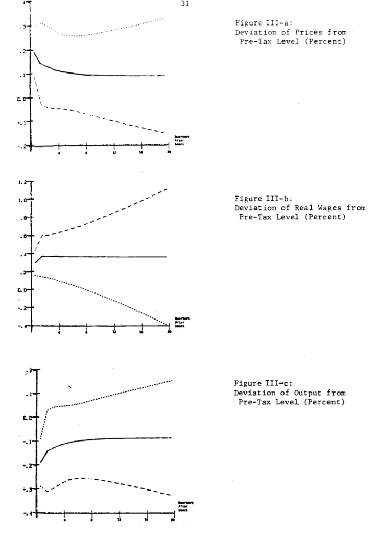
The estimates from system (io) also suggest significant tax effects, as

can be seen from the impulse response functions in Figure III. Prices rise

by .19 percent in the quarter of the shock,

forty percent of the amount which

would be predicted if pre—tax prices were

completely fixed. They decline slowly

thereafter, and are still more than .08 percent

above their initial

I I I

4 4 I? *4 a

Figure 111—a:

Deviation of Prices from Pre—lax Level (Percent)

Figure Ill—b:

Deviation of Real Wages from Pre—Tax Level (Percent)

Figure III: Estimated Impulse Responses to a One Percent TNIX Shock Estimates for Great Britain based on System (10)

31

V

— 1.21 1. .8

-/

C.D *tIl 4 S U is a

.?'

/

::

-3•

,..-.-Figure III-c:

Deviation of Output from Pre—Tax Level (Percent)

3:

level four years afterwards. The standard errors for the impulse response functions from (io) are however larger than those from (9). Five quarters after the tax change, the sum of the deviation of prices from their initial level is .655 percent, with a standard error of .710. Real wages again rise for a short while after the tax shock occurs, and then decline. Output changes in this system, which are equal to the negative of the price

impulses, display a more stable response pattern than those in system (9). We explored the robustness of our tax mix results in several ways. We

._1... .__.._ 4.

ia

be

.±

4...1 L1..._. 4.L

ey

statistically

insignificant coefficients and did not affect our conclusions about tax policy. We continued to reject the null hypothesis of zero

coefficients

on the tax mix

variables at

very high levels. We also estimated

our

equations without

the indicator variables for wage and price controls,

and most

of the tax coefficients changed very little. Adding further lagged

variables to the system reduced the statistical significance of some

coefficient estimates, but had little iact on either our estimated dynamic responses or our rejections of the tax neutrality hypothesis.25

IV. C. United States TNIX Results

In this section, we investigate wflether our U.K. findings are

consistent

with the U.S. experience. Appendix Table A—3 presents estimates of systems

(9) and (10) using American data for the 1955:1—1984:3 period. The central question is whether we can reject the null hypothesis that TMIX should be

25•

A change in the total tax burden also has real effects. In the three—

equation

system,

a one

percent

of GDP

increase in the

total tax

burden reduces output .51 percent in the quarter of the tax change, and induces lower

output

for three quarters after the shock. The

estimates

of TTOT's

iact

on both prices and output, however, are plagued by

very large

standard

33

excluded from these systen.is. For

system

(9),

the

test statistic is 21.7.

Since it is aistributed X2(6) uncer the short-run tax neutrality hypothesis, this constitutes a rejection at

tue .01 level.

For system (10), the two— equation system, the test statistic of 17.8 (2(4) under the null) also implies rejection at the .01 level. These findings provide strong evidence for the presence of wage or price stickiness in the United States. To illustrate effects which these rigidities imply for tax changes, we now consider impulse response functions for prices, wages, and output. In both systems, we clearly reject the null hypothesis that the tax mix variables have zero coefficients. The test statistics again imply rejections at the

.01 level. Our discussion will focus

on

estimates which use the GNP deflator to measure prices. Using the shelter—exclusive CPI, however, yields even stronger rejections of the tax

irrelevance

hypothesis and even more

pronounced price effects after a tax change.

Figures IV and V report the impulse response functions corresponding to systems

(9)

and

(i o). The

initial effect of a permanent one percent

TMIX

increase is a .32 percent increase in prices. As in tne british data, prices

continue to increase for one quarter after the tax shock, and

decline

smoothly

thereafter. The absence of significant tax

variation

makes the

standard

error on

the estimated price responses larger than those for

Britain. The sum of the price changes for the first five quarters after the

change is 1.130, with a standard error of 1.63. The Arican evidence also

differs from the British in suggesting much

slower adjustment

back to

equilibrium, as is clear from Figure IV.

Real wages also rise after a tax shock, corroborating our British

findings. The initial effect of a one percent TMIX shock is to raise the

Ii

_f:r'

Figure IV—a:

Deviation of Prices from Pre-Tax Levels (Percent)

Figure IV—c:

Deviation of Output from Pre—Tax Levels (Percent)

Figure IV: Estimated Impulse Responses to a One Percent TMIX Shock Estimates for the United States, based on System (9)

34 /

I

/

:_

c-c. U 1.0-Figure IV—b:

Deviation of Real Wages from Pre—Tax Levels (Percent)

0.0

I I

4 4 U II N

Figure V—a:

Deviation of Prices from Pre—Tax Level (Percent)

1.0

—

isa

4

I

U *4 40

,

"

Figure V—b:

Deviation of Real Wages from Pre—Tax Level (Percent)

—.I---f---t----i

4 I _{Ii II} - _N

Figure V: Estimated Impulse Responses to a One

Percent

TMIX Shock Estimates for United States based on System (10)

35 .5_

0.0

I'

I'

.8-tm

1— C. C —. I— —.3— —. —.5. Figure V—c:

Deviation of Output from Pre—Tax

Level (Percent)

additional quarter, and then decline monotonically to their initial level. Adjustment is slow; even five years after the tax shock, real wages are .13 percent above their initial level.

Output experiences a pronounced decline after an increase in indirect taxation. A one percent rise in TMIX induces a .2 percent drop in real GNP in the quarter of the tax change. The path of output thereafter depends upon the choice between systems (9) and (10). In (9), the three equation system, output continues to decline for another quarter and falls to .45 percent below its initial level before starting to return to its initial level. The sum of the output effects up to ten quarters after the change is —4.120, with a standard error of 2.731. The results for (10) suggest that the amount of lost output declines after the first quarter, although output returns to its initial level very slowly. The ten—quarter sum equals —2.903 (2.951). Both sets of results are consistent with the view that nominal wages are sticky, since the insufficient nominal wage decline in response to indirect tax

increases raises real wages and induces firms to lay off workers. This has the ultimate effect of lowering real money balances.

Our

findings

are insensitive to several specification changes.

Fcluding Gordon and King's (1982) wage—price control variables has little effect on the e'stimated coefficients and iipulse response functions. Adding interest rates, exchange rates, and further lagged values of the currently included variables also has little substantive impact on our conclusions. The central finding, that the short—run tax neutrality hypothesis is strongly rejected, obtains in a wide variety of specifications.

These results can also be used to study the inact of revenue—raising tax increases. Raising the total tax burden permanently, while keeping TMIX constant, increases prices and real wages and causes a drop in output. A one

37

percent increase in TTOT raises prices by .38 percent, and real wages by .26 percent, in the first quarter. itput declines by .8 percent when the shock occurs, and continues to fall thereafter. By

eight

quarters after tne tax increase, output is 1.65 percent below its starting value. These findings, while suggestive, are accompanied by large standard errors and should

therefore be interpreted with caution.

IV.

D.

Qualifications

Pwo potentially important assuniptions underlie our use of the TMIX variable to test for the existence of nominal rigidities. First, we assume that TMIX is exogenous in our reduced form equation systems. Second, we postulate

that except for the effects of wage and price stickiness, changes

in

TMIX should have no iact on prices or output. The possible failure of parallel assumptions has caused

debate about the interpretation of linkages

between money

and output. We consider each assuition in turn.

Several arguments might be constructed to suggest that our tax mix

variable is not exogenous. Perhaps most plausibly, it might be noted that if the output elasticities

of direct and indirect taxes are different, then

changes

in

real output will induce changes in TiiIX. Price shocks may be transmitted to'GNP and

tnen to TNIX as

well. This issue is partly addressed by our inclusion of lagged output in the reduced form systems, and by our separate examination of the 1979 and 1976 policy changes in Great Britain. As a further check, we use data on cyclically adjusted revenue collections26

26•

Full

employment data are not available for the U.K. on a quarterly basis. In the United States, data on federal taxes beginning in 1955 are published in Halloway (1984a, 1984b). Ftimates of high employment state and local

receipts were constructed by the authors.

to create full employment TMIX and TTOT variables for tne United States. These data were only available for the post—1955 period. The results obtained using tnese variables were similar to those obtained with our unadjusted tax variables, suggesting that cyclical fluctuations are not an important source of endogeneity for the receipts—based tax measures.27

Unfortunately, the data are not available to examine the effects of cyclical adjustments for Great Britain, or for the entire post-1948 period in the

United States.

An

alternative arj.ment against

_{the exogeneity of TMIX might hold that}

the

tax

mix is set in response to projected economic

conditions, or that it

helps

to forecast future economic policies. Consideration of the historical context which generated changes in TMIX does not support these views. The 1979 tax reform in Great Britain immediately followed an election which was decided on grounds other than tax policy. The avowed purpose of its

proponents was to improve incentives through reductions in marginal income tax rates. In the United States, most of the variation in indirect taxes comes from movements in state sales taxes and employer payroll taxes. Neither of these are likely to be manipulated for macroeconomic purposes. More generally, it seems unlikely that governments systematically shift towards indirec't taxes when they foresee rising prices, or when they intend to pursue more expansionary monetary policy. The 1979 re(orrn in Britain was accoan.ied by an announced policy of monetary restraint. Nothing in the

27• Although the results using full employment and unadjusted TMIX are always similar, the resemblence between our equations for the 1948—1984 period (reported in Table A-.3) and the coirarison equations for 1955—1984

depended upon our choice of price series. The equations using the shelter— exclusive CPI are very similar to those for the full sample period, while those using the GNP deflator are substantially different.

59

history of eitner British or American tax policy suggests that tax changes should help to forecast future monetary policies. This inference is

consistent with the failure of Granger causality tests to reject the hypothesis that TMIX does not cause either money or TTOT.

The second potential objection to our tests is that TMIX might have effects on output and prices through channels other than wage and price

rigidities. Such a possibility cannot be ruled out, since changes in TMIX do not correspond precisely to our theoretical model. Indirect taxes do not

cover all goods, and direct taxes are not strictly proportional.

Nonetheless, it is difficult to explain our findings along these lines. Increases in indirect taxes coupled with equal revenue decreases in direct taxes are usually though to improve incentives to work and invest. Since indirect taxes are also less progressive than direct taxes, they should have smaller disincentive effects. Thus, they should raise output and reduce prices ——

the

opposite of what we find.

There are no controlled experiments in macroeconomics. Nevertheless, we find it

difficult

to account for our results in

terms

_{of the limitations of}

tax—shift experiments. At a ininimuzii, the flaws in our tax—based tests are

largely independent of those in tests which focus on the relationship between

money and outpt. Hence, our tests

provide at least some additional evidence

40

V. Conclusions

A major thrust of much recent macroeconomic research has been the elucidation of business cycles as equilibria of competitive economies with fully flexible prices. Theories in both the "misperceptions" and "real business cycle" traditions emphasize the assption of perfect price flexibility and the resulting absence of unexploited opportunities for beneficial exchange. These theories imply strong data restrictions: fully perceived changes in government policy which do not change any agent's opportunity set should have no real effects. In contrast, the essence of contemporary Keynesian thinking is ttiat prices are in some sense sticky, so certain purely nominal disturbances ao matter.

The difficulty in exirically distinguishing these theories arises from the problem of isolating purely nominal disturbances. Traditionally, they have been tested by examining the relationship between variously—measured monetary shocks and real variables. These tests have not been entirely conclusive because a variety of rationalizations, with very

different

structural implications, can be offered for the comovement of money and

output.

In this paper, we rely on tax shocks of a special sort to distinguish between classi&al and Keynesian models. A clear implication of microeconoxxiic theory with flexible prices is that the side of the market on which a tax is collected does not influence its ultimate real effects. Tax changes between direct

and indirect taxation therefore provide a natural experiment for

examining the importance of nominal rigidities. The appeal of the experiment

is enhanced by the apparently unsystematic way in which taxes

have

varied.

The results of our investigation lead us to decisively reject the

44

may be made

to

rationalize the comovements we observe with perfectly flexible

prices, we find it impossible to convincingly account.

for

_{the empirical} regularities in the data without asstining some sort of price rigidity.

Asserting

that

prices are rigid falls far short of explaining them or understanding

their properties. Our results suggest that this remains a

vitally

important research problem. "Menu costs," which have been proposed as one explanation for price rigidities, cannot explain why many prices which can be changed costlessly, such as newstand magazine prices,28 appear to

change infrequently. Moreover. moneta policy appears potent even in highly inflationary economies, where menu costs

should be less important.

Our results

have potentialir important consequences for tax

policy.

Almost universally, reforms in the tax structure are evaluated within the context of market clearing

models where prices

_{are perfectly flexible.}

Within such models, the distinction between direct and indirect taxation is of no consequence. Our

findin

suggest that

this distinction may be

important over periods of

several years, during which prices are sticky.

Indeed

the macroeconomic consequences of some reforms may

dwarf

their

microeconoxnic

iact on economic efficiency.

If unemployment is a

significant byproduct of certain tax reforms, traditional thinking about their incidence needs to be reconsidered.

Consider as an example current proposals to raise revenue by taxing domestic and imported crude oil. Available estimates29 suggest that this

28• Cechetti (1984) presents detailed evidence on the inflexibility of

magazine prices.

42

measure would raise about 4.2 billion dollars for each one dollar per barrel tax. Thus a five dollar a barrel tax would raise the indirect tax burden by 21 billion dollars. Our estimates suggest that if monetary policy were not altered, this would result in lost output of sixty billion dollars

over the succeeding decade. Similar estimates are obtained assuming that monetary policy acts to keep nominal GNP constant following the tax reform. These figures bulk large relative to allocative effects traditionally

enthasized in microeconomic analyses of excise tax reforms. Proposals to tax only marginal suppliers of goods, such as the proposed surtax on oil imports, would have much greater output effects per dollar of revenue raised.

Some might argue that it is inappropriate to assess the output effects of tax reforms while holding monetary policy constant, since monetary policy could accommodate tax changes. This issue is treated in Poterba, Rotemberg and Summers (1985). Note, however, that if the monetary authority has set monetary policy to trade off unemployment and inflation in a desirable way prior to tax reform, the loss of welfare from a small tax change will be independent of the monetary policy response. Unless one believes that monetary

policy

is wrong prior to a tax reform, there is no reason not to

evaluate

the effects of the tax

holding

monetary policy constant. This is especially

true

for small reforms such as the

gasoline tax. It

is

also

inconceivable that

the effects of small reforms could be disentangled

accurately enough for them to be explicitly accommodated by monetary policy. Our finding

that shifts towards indirect taxation have adverse

macroeconomic consequences raises an obvious question. Could macroeconomic

performance be improved by reducing indirect taxes and increasing direct

taxes? The conscious and regular use of such tax policies as

stabilization

4

estimates cannot shed much light on this issue. However, they do suggest that such a change might well improve the tradeoff between unemployment and inflation on a one-shot basis. The gains might be taken either in the form of reduced inflation or increased output. Poterba, Rotemberg and Summers

(1985) demonstrate that if output is held constant, tax changes may well have a permanent effect on the rate of inflation.

Our results suggest a number of directions for future research. The robustness of our conclusions might be examined by studying tax changes in other countries or in individual American states. Structural estimation might yield more precise information on the nature of wage and price stickiness, and

tax

reforims might facilitate identification of these

models. The effects of alternative policy responses to large tax reforms might also be considered. Perhaps most importantly, our results isolate a major class of apparent rigidities which economic theory needs to explain.

44

he fe ren ce s

Blanchard, Olivier J., 1983, Price desynchronization and price level inertia, in R. Dornbusch and M. Simonsen (eds.), Inflation, Debt, and Indexation, MIT Press, Cambridge, ?A.

Blanchard, Olivier J., 1985, The wage price spiral, MIT

mimeo.

Blinder, Alan S., 1973, Can income taxes be inflationary? An expository note, National Tax

Journal,

26, 295-301.

Blinder, Alan S., 1981,

Monetary accommodation

of supply shocks under rational expectations, Journal of Money, Credit, and Banking 13, 425— 38.

Branson, William and Julio Rotemberg, 1980, International adjustment with wage

rigidity, European Economic Review 13, 309-332.

Break, George 11.,

1974, The incidence

and economic effects