Multiproduct Intermediaries

Multiproduct Intermediaries

Andrew Rhodes

Toulouse School of Economics

University of Toulouse Capitole

Makoto Watanabe

Department of Economics

VU Amsterdam

Jidong Zhou

School of Management

Yale University

May 2020

This paper develops a new framework for studying multiproduct intermediaries when consumers demand multiple products and face search frictions. We show that a multiproduct intermediary is pro…table even when it does not improve consumer search e¢ ciency. In its optimal product selection, it stocks high-value products ex-clusively to attract consumers to visit, then pro…ts by selling non-exclusive products which are relatively cheap to buy from upstream suppliers. However, relative to the social optimum, the intermediary tends to be too big and stock too many products exclusively. As applications we use the framework to study the optimal design of a shopping mall, and the impact of direct-to-consumer sales by upstream suppliers on the retail market.

Keywords: intermediaries, multiproduct demand, search, direct-to-consumer sales, product range, exclusivity

JEL classi…cation: D83, L42, L81

We are grateful for helpful comments to the Editor and an anonymous referee, as well as Mark Armstrong, Heski Bar-Isaac, Alessandro Bonatti, Joyee Deb, Paul Ellickson, Doh-Shin Jeon, Bruno Jullien, Fei Li, Barry Nalebu¤, Martin Obradovits, Rob Porter, Jerome Renault, Patrick Rey, Mike Riordan, Greg Sha¤er, Andy Skrzypacz, Guofu Tan, Greg Taylor, Raphael Thomadsen, Glen Weyl, Mike Whinston, Chris Wilson, Julian Wright and seminar participants in Bonn, Cambridge, Cornell, Durham, HKUST, MIT, MSU, NUS, NYU Stern, Oxford, Stanford, Tokyo, TSE, UC Davis, UCL, UCLA Anderson, UIUC, USC, Yale, Zurich as well as the 8th Consumer Search and Switching Workshop, Bristol IO Day, EARIE, EEA (Lisbon), ICT conference (Mannheim), SAET (Faro), SICS (Berkeley), TNIT (Microsoft), the 16th Annual Columbia/Duke/MIT/Northwestern IO Theory Conference, and the 19th CEPR IO Conference. Rhodes gratefully acknowledges funding from the European Research Council (grant No 670494) and the Agence Nationale de la Recherche (grant ANR-17-EURE-0010).

1

Introduction

Intermediaries are important players in the economy.1 _{Many intermediaries carry multiple}

di¤erent products, and serve buyers with multiproduct demand. Examples include retail-ers such as supermarkets and department stores, shopping malls, TV platforms, travel agencies, and trade intermediaries. However much of the existing literature focuses on single-product intermediaries. Our paper builds a new framework to study multiproduct intermediaries when consumers demand multiple products and have search frictions. We then use this framework to address several important questions. For example, how can a multiproduct intermediary create value and therefore pro…tably exist? Which products should the intermediary carry, and for which of them should it be the exclusive supplier in the market? Surprisingly there is very little existing research about this, even though in practice the decision of which products to carry is one of the most important choices faced by intermediaries.2 _{We also ask, is the intermediary too big or too small relative}

to the social optimum, and does it carry qualitatively the ‘right’products? Further, it is increasingly easy for sellers to bypass traditional intermediaries and sell direct to buyers. What are the possible consequences of this new trend, and how should intermediaries respond?

Our framework can shed light on some important developments in retail (and other intermediary) markets. Traditionally, most manufacturers could only reach consumers via retailers. However in recent years this has changed. Manufacturers of many di¤erent types of product now sell direct-to-consumer (DTC).3 A survey by the European Commission (2017) found that the percentage of EU manufacturers selling direct is as high as 85% in clothing and shoes, and above 50% in …ve other product categories. Many established brands like Nike and Nestle sell direct via their own website or physical store, while smaller brands do so via online marketplaces like Amazon and Tmall.4 _{(Direct sales are}

1_{Krakovsky (2015) suggests that middlemen are responsible for around one third of US GDP.} 2_{Writing in the Harvard Business Review, Fisher and Vaidyanathan (2012) argue that successful}

retailers must be “good on a number of dimensions... But assortment is number one.” A good product assortment is crucial for attracting shoppers, who are often time-constrained and therefore shop at a few retailers whose product range closely meets their needs. At the same time, even large retailers like Walmart cannot stock all products desired by consumers, either due to space constraints, or because stocking too many products makes the instore shopping experience less pleasant.

3_{As an example, in 2017 DTC wine sales in the US were worth $2.7 billion, almost 10% of the total}

(US) market (see https://bit.ly/30qNQVq). DTC sales are also becoming popular in industries such as traditional packaged goods, consumer electronics, and travel services (see https://bit.ly/2VKiB8e).

4_{Nike’s DTC sales in 2017 were worth $10.4 billion, and it set itself the goal of increasing them to}

$16 billion by 2020 (see https://on.wsj.com/2ITY5wN and https://bit.ly/2DgV706). According to the European Commission (2017), 20% of respondent manufacturers sell via marketplaces. Meanwhile the consulting …rm Oliver Wyman (2018) found that more than half of US online sales of general merchandise in 2016 were direct (via either the manufacturers’own websites or marketplaces).

also gaining traction in other markets, such as those for TV platforms.) Commentators have argued that DTC will grow further in the coming years and risks undermining traditional retailers’one-stop shopping business model. Some have even linked DTC to the closure of certain retailers and the sluggish performance of others.5 _{Our paper o¤ers}

a framework in which to assess these claims, and to study how retailers should respond as DTC sales become more prevalent.

Another important trend in retail markets is exclusivity. Exclusivity agreements be-tween manufacturers and retailers are increasingly common, and already exist for a wide variety of products including toys, furniture, and even groceries.6 _{Macy’s has signed}

ex-clusive deals with several brands, and set itself the goal of increasing the percentage of products that are unique to its stores from 29% in 2017 to 40% in 2020. Similarly, Tar-get is well-known for its exclusive deals with designers of apparel and homeware.7 Our paper o¤ers a framework to think about the incentives to enter into exclusivity arrange-ments, which products should be stocked exclusively, and how DTC and other changes in technology may a¤ect the propensity to use exclusivity agreements.

Section 2 of our paper introduces the baseline model. It is mainly developed for retailers but, as we discuss later, the setup and some of the main insights also apply to a broader set of multiproduct intermediaries including shopping malls, TV platforms, and trade intermediaries. There is a unit mass of manufacturers, each of which produces a di¤erent product. Consumers view these products as independent and are interested in buying all of them. Consumers have the same demand for a given product, but di¤erent products have di¤erent demands. There is also one multiproduct intermediary. A product can be sold to consumers either directly by the manufacturer, or by the intermediary, or through both these channels. The intermediary compensates a manufacturer whose product it carries by way of a two-part tari¤, and can request exclusive sales rights. The intermediary may also be limited in how many products it can stock. Consumers must incur a search cost to learn a seller’s price(s) and buy its product(s), and the search cost is proportional to the time needed to visit it. We normalize the time needed to search a measure one of manufacturers to one, and assume the time needed to search the intermediary is weakly increasing in how many products it carries. (In the retail example, the latter would be consistent with the idea that larger retailers are located further from consumers, or are harder to navigate.) An important feature of our model is that consumers di¤er in their cost of time and so di¤er in their search cost.

Since the focus of our paper is product range choice, we intentionally simplify

sell-5_{See for example https://on.wsj.com/2V2i6lx and https://bit.ly/2DgV706, and also Section 6.} 6_{A survey by GfK (2007) for the UK Competition Commission found that 35% of grocery-product}

suppliers had been asked to enter an exclusivity agreement, and 19% had done so. Gielens et al (2014) give examples of exclusive products by well-known manufacturers like Procter and Gamble and Unilever.

ers’ pricing problems. In our model, irrespective of the market structure each supplier of a given product always charges the usual monopoly price.8 _{We then argue that all}

information about a product’s cost and demand curve can be summarized using a simple two-dimensional statistic ( ; v), where represents a product’s monopoly pro…t and v

represents its monopoly consumer surplus. This enables us to study product range choice in a tractable way, since it reduces a potentially complicated product space into a simpler two-dimensional one. Speci…cally, the intermediary’s problem is to choose a set of points within the ( ; v) space that it will stock exclusively, and another set of points which it will stock non-exclusively.

In Sections 3 and 4 we solve for the intermediary’s optimal product range, …rst in a simple case to provide some initial intuition, and then in the general case. Unlike the standard single-product case, we show that a multiproduct intermediary can earn strictly positive pro…t even when it does not improve consumer search e¢ ciency. The underly-ing mechanism is related to the classic bundlunderly-ing argument, and it relies on consumers’ multiproduct demand and heterogeneous search costs and the availability of exclusive contracts. We also show that the value from stocking a product can be split into a ‘direct’ and ‘indirect’ component. The direct component represents the pro…t earned through selling that product. It includes compensation paid to the manufacturer and can there-fore be negative. The indirect component re‡ects cross-product externalities i.e. the way in which stocking a new product may either increase or decrease how many consumers search the intermediary, and thereby change the pro…tability of the intermediary’s other products.

The optimal stocking policy itself consists of three distinct ‘regions’in the( ; v)space. Firstly, the intermediary stocks some products with high-v but low- exclusively. These products make a direct loss but they help attract consumers due to their highv.9 Secondly, the intermediary recoups these losses by stocking some other very pro…table products with low-v but high- . However since these products have lowv they may dissuade consumers from searching, and so in general the intermediary avoids stocking too many of them. Thirdly, depending on the intermediary’s stocking constraint and search technology, it may also stock some products with high-v and high- non-exclusively. These products break even but can have a positive indirect e¤ect. Compared to the social optimum, we argue that the intermediary tends to stock too many products, and to stock too many of

8_{Intuitively, with two-part tari¤s the intermediary buys marginal units from a manufacturer at cost.}

Given that consumers have homogeneous preferences and do not observe price before search, the logic of Diamond (1971) then implies that there is no price competition even if a product is sold by both its upstream supplier and the intermediary. As we discuss more in Section 2, the monopoly pricing itself is not crucial for our analysis - what matters is that the price of each product is the same across sellers.

9_{The result that exclusive products help attract consumers to visit but may incur a loss for the}

retailer is similar to, but di¤erent from, the usual loss-leader argument. Here the loss is due to the high compensation required by the manufacturer, instead of below-cost pricing.

them exclusively. Nevertheless the intermediary can be welfare-enhancing due to the way it a¤ects consumers’incentives to search.

Section 5 studies two applications of our framework. Section 5.1 discusses the optimal design of a shopping mall which acts as a platform and does not directly resell products. Our framework provides insights about which shops should join the mall and how much they should pay to do so, as well as the externalities they exert on other shops. Section 5.2 applies our framework to DTC sales. When DTC sales become easier the intermediary has to compensate manufacturers more for stocking their products, and so not surprisingly manufacturers are better o¤ but the intermediary is worse o¤. More importantly, we also show that the intermediary should respond to easier DTC sales by stocking fewer products, but stocking a greater proportion of them exclusively. As we explain in more detail later on, we also …nd that the optimal product selection becomes more ‘polarized’ in the( ; v)space, and both a product’s easiness to be sold direct and its location in the ( ; v)space a¤ect whether (and how much) its direct sales take o¤. Moreover, easier DTC sales in one sector can induce manufacturers in other (una¤ected) sectors to also sell more direct, due to a spillover e¤ect. Finally, we show by example that if the intermediary fails to adjust its product selection in this way, it can end up with negative pro…t and thus have to exit the market altogether.

The remainder of the paper is then structured as follows. Section 6 provides evidence for the key economic forces in our model and its main predictions. In Section 7 we …rst provide a foundation for the ( ; v) product space and interpret di¤erent points within it. We then present two extensions and show that our main insights are qualitatively robust to demand heterogeneity and upstream competition. Finally Section 8 concludes and discusses the potential application of our framework to other types of intermediary. All proofs are available in the Online Appendix.

1.1

Related literature

There is already a substantial body of literature on intermediaries (see e.g. the book by Spulber (1999)). An intermediary may exist because it improves the search and match-ing e¢ ciency between buyers and sellers (e.g. Rubinstein and Wolinsky (1987), Gehrig (1993), Spulber (1996), and Shevchenko (2004)), or because it acts as an expert or certi-…er that mitigates the asymmetric information problem between buyers and sellers (e.g. Biglaiser (1993), Lizzeri (1999), and Biglaiser and Li (2018)).10 We study intermediaries in an environment with search frictions, but in our model an intermediary can pro…tably exist even if it does not improve search e¢ ciency. Our model features consumers

demand-10_{Other reasons why retailers in particular may exist are i) they know more about consumer demand}

than manufacturers do, ii) they can internalize pricing externalities when products are substitutes or complements, and iii) they may be more e¢ cient in marketing activities due to economies of scale.

ing multiple products and having heterogeneous search costs and the possibility of using exclusive contracts.11 _{These features distinguish our model from existing work on}

inter-mediaries. Since our main focus is the retail market, we also study optimal product range and the impact of DTC sales, neither of which are typically addressed by the intermediary literature.

The mechanism by which an intermediary makes pro…t from stocking multiple prod-ucts is reminiscent of bundling (e.g. Stigler (1968), Adams and Yellen (1976), McAfee et al (1989), and Chen and Riordan (2013)). By stocking some products that consumers value highly but are not available elsewhere, the intermediary induces consumers to visit and buy other low-value (but fairly pro…table) products as well which consumers would other-wise not buy. However since our paper focuses on product selection, it is more related to the question of which products a …rm should bundle, something which is rarely discussed in the bundling literature. Rayo and Segal (2010) use the same bundling argument in a di¤erent setting with information design. They show that an information platform often prefers partial information disclosure, in the sense of pooling two negatively correlated prospects into one signal. (For example a search engine may pool a high-relevance but low-pro…t ad with a low-relevance but high-pro…t ad.) Unlike us, they consider a discrete framework and (more importantly) they allow the information platform to send an arbi-trary number of signals (which in our framework, would be like allowing the intermediary to organize and sell non-overlapping products in multiple stores). Consequently their op-timization problem is very di¤erent from ours. Moreover many other important features of our model, such as the role of exclusivity and the importance of search economies, have no counterpart in their paper (or in the wider bundling literature).

Our paper is also related to the growing literature on multiproduct search (e.g. McAfee (1995), Shelegia (2012), Zhou (2014), Rhodes (2015), and Kaplan et al (2019)). Existing papers usually investigate how multiproduct consumer search a¤ects multiproduct retail-ers’pricing decisions when their product range is exogenously given. Our paper departs from this literature by focusing on product range choice, another important decision for multiproduct retailers.12 _{Moreover our paper introduces manufacturers and so explicitly}

models the vertical structure of the retail market. In this sense it is also related to recent research on consumer search in vertical markets such as Janssen and Shelegia (2015), and Asker and Bar-Isaac (2020), although those works consider single-product search and address very di¤erent economic questions.

Finally, our paper is also related to research on product assortment in operations

11_{In Spiegler (2000) two agents create surplus when they interact. A third party which does not improve}

e¢ ciency can extract this surplus through “exclusive-interaction” contracts, which force the agents into a Prisoner’s Dilemma. Our paper studies a very di¤erent type of exclusivity arrangement.

12_{Rhodes and Zhou (2019) also study retailers’endogenous product range, but they consider a stylized}

research and marketing (see e.g. the survey by Kök et al (2015)). Typically this literature focuses on a situation where consumers demand a single product, and studies the optimal number of (symmetric) varieties of that product to stock. Our paper focuses instead on a retailer’s optimal product range choice when consumers have multiproduct demand. We study this issue with explicit upstream manufacturers and consumer shopping frictions, neither of which is usually considered in the above mentioned literature.13

2

The Model

There is a continuum of manufacturers with measure one, and each produces a di¤erent product. Manufacturer i has constant marginal cost ci 0. There is also a unit mass of consumers, who are interested in buying every product. The products are independent, and each consumer wishes to buy Qi(pi) units of product i when its price is pi. When a consumer buys multiple products, her surplus is additive over these products. We assume that Qi(pi) is downward-sloping and well-behaved such that (pi ci)Qi(pi) is single-peaked at the monopoly price pm

i . Per-consumer monopoly pro…t and consumer surplus from product i are respectively denoted by

i (pmi ci)Qi(pmi ) and vi

Z 1

pm i

Qi(p)dp. (1)

Manufacturers can sell their product direct to consumers, for example via their own retail outlet.14 In addition there is one multiproduct intermediary, which can buy products from manufacturers and resell them to consumers. The intermediary has no resale cost, but can stock at most a measurem 1of the products. We assume that the intermediary has all the bargaining power, and simultaneously makes take-it-or-leave-it o¤ers to each manufacturer whose product it wishes to stock.15 _{These o¤ers can be either ‘exclusive’}

(meaning that only the intermediary can sell the product to consumers) or ‘non-exclusive’ (meaning that both the intermediary and the relevant manufacturer can sell the product to consumers). In both cases we suppose that the intermediary o¤ers two-part tari¤s, consisting of a wholesale unit price i and a lump-sum fee Ti. The intermediary also informs manufacturers about which products it intends to stock, and whether it intends

13_{Bronnenberg (2020) considers a model where consumers like variety but dislike shopping, so retailers}

stock multiple varieties to reduce consumers’shopping costs. His model is otherwise very di¤erent from ours, as are the questions it studies. For example in his model varieties are symmetric, and so he does not look at the optimal composition of a retailer’s product line.

14_{Alternatively, we can interpret direct sales as a manufacturer selling through an independent specialist}

retailer. If the manufacturer can make a take-it-or-leave-it two-part tari¤ o¤er to the specialist retailer, all our analysis and results remain unchanged.

15_{Our results do not change qualitatively if instead the intermediary and manufacturer share any pro…ts}

to stock them exclusively or non-exclusively.16 Manufacturers who received an o¤er then simultaneously accept or reject.

Consumers know where each product is available, but do not observe the terms of any upstream contracts. Moreover consumers cannot observe a …rm’s price(s) or buy its product(s) without incurring a search cost.17 _{Consumers di¤er in terms of their ‘unit’}

search cost s, which is distributed in the population according to a cumulative distri-bution function F(s) with support (0; s]. The corresponding density function f(s) is everywhere di¤erentiable, strictly positive, and uniformly bounded with maxsf(s)<1. If a consumer searches a measurenof manufacturers, she incurs a total search cost n s. If a consumer also searches the intermediary, and the intermediary stocks a measurem of products, she incurs an additional search cost h(m) s. We can thus interpret s as the opportunity cost of time, with the time needed to visit a measure one of manufacturers normalized to 1, and the time needed to visit the intermediary equal to h(m).18 We assume that the function h(m) is positive and weakly increasing, re‡ecting the idea that larger stores may take longer to navigate, and may also be located further out of town. (Notice that we allow for the case where h(m) is constant and so independent of the intermediary’s size. Below we provide a microfoundation for why h(m) might be strictly increasing.) We also introduce the following notation: when h(m)< mthe intermediary generates economies of search, and when h(m)> m it generates diseconomies of search. Finally as is standard, we assume that after searching consumers may costlessly recall past o¤ers.

The timing of the game is as follows. At the …rst stage, the intermediary simulta-neously makes o¤ers to manufacturers whose product it would like to stock. An o¤er speci…es i and Ti and whether the intermediary will sell the product exclusively or not. Manufacturers then simultaneously accept or reject. At the second stage, all …rms that sell to consumers choose a retail price for each of their products. The intermediary uses linear pricing. At the third stage, consumers observe who sells what and form (rational) expectations about all retail prices. They then search sequentially among …rms and make their purchases. We assume that if consumers observe an unexpected price at some …rm, they hold passive beliefs about the retail prices they have not yet discovered.

2.1

Preliminary analysis

16_{This assumption aims to capture the idea that in practice negotiations evolve over time, such that}

manufacturers can (roughly) observe what other products the intermediary stocks.

17_{Our assumptions here try to capture the idea that a retailer’s product range is usually reasonably}

steady over time, whilst its prices are easier to adjust.

Lemma 1 (i) In any equilibrium where each product market is active, each seller of a product charges consumers the relevant monopoly price.

(ii) If product i is stocked exclusively by the intermediary, the intermediary o¤ers the manufacturer a wholesale unit price i = ci and a lump-sum payment Ti = iF (vi). If product i is stocked non-exclusively by the intermediary, in terms of studying the opti-mal product range, it is without loss of generality to focus on the contracting outcome where the intermediary o¤ers the manufacturer i =ci and Ti at a level that ensures the manufacturer’s total payo¤ is iF (vi).

To understand the intuition behind Lemma 1, recall that a product can be sold in three di¤erent ways. Firstly producti may be sold only by its manufacturer. Consumers then face a standard hold-up problem (see e.g. Stiglitz (1979) and Anderson and Renault (2006)). Since consumers only learn the manufacturer’s price after they have sunk their search cost, the manufacturer optimally charges the monopoly price pm

i .19 Consumers rationally anticipate this and therefore search if and only if s vi. Consequently the manufacturer earns a pro…t iF (vi). Notice that this is also the manufacturer’s outside option if the intermediary makes it an o¤er.

Continuing with the intuition for Lemma 1, secondly productimay be sold exclusively by the intermediary. Since consumers do not observe the price before searching, the same hold-up argument implies that if the intermediary faces a wholesale price i, it will charge the corresponding monopoly price arg max (p i)Qi(p). Notice that joint pro…t earned on product i is maximized when the intermediary charges the monopoly price pm_i , therefore in order to induce this outcome the intermediary proposes i = ci i.e. a bilaterally e¢ cient two-part tari¤. The intermediary then drives the manufacturer down to its outside option by o¤ering it a lump-sum payment Ti = iF (vi). Thirdly product imay be sold by both its manufacturer and the intermediary. The analysis here is subtler. Intuitively the intermediary again avoids double-marginalization by proposing a contract with i = ci, whilst search frictions eliminate price competition between the manufacturer and intermediary. In particular, following Diamond’s (1971) paradox if consumers expect both sellers to charge the same price for product i, they will search at most one of them and hence each …nds it optimal to charge the monopoly price. The manufacturer is compensated for any sales that it loses in signing the contract by way of a lump-sum transfer.

Given Lemma 1, it is convenient to index products by their per-consumer monopoly pro…t and consumer surplus as de…ned in (1) (rather than by their demand curveQi(pi) and cost ci). This helps convert the potentially complicated product space into a two-dimensional one. Henceforth let _R2+ be a two-dimensional product space ( ; v), and

19_{As is usual in search models, there also exist other equilibria in which consumers do not search (some)}

sellers because they are expected to charge very high prices, and given no consumers search these high prices can be trivially sustained. We do not consider these uninteresting equilibria in this paper.

suppose it is compact and convex. Letv 0andv <₁be the lower and the upper bound of v. For each v ₂ [v; v], there exist 0 (v) (v) < ₁ such that ₂ [ (v); (v)]. (In Section 7.1 we provide examples of demand functions which can generate this type of product space.)

Let ( ;_F; G) be a probability measure space where _F is a -…eld which is the set of all measurable subsets of according to measure G. (In particular, G( ) = 1.) When there is no confusion, we also use G to denote the joint distribution function of ( ; v), and let g be the corresponding joint density function. We assume thatg is di¤erentiable and strictly positive everywhere. If a consumer buys a set A _{2 F} of products at their monopoly prices, she obtains surplus R_AvdG before taking into account the search cost. To avoid trivial corner solutions, we also assume that v s.

Discussion. Before solving for the intermediary’s optimal product range, we …rst discuss some of our modeling assumptions and their implications.

(i) A continuum of products. Considering a continuum of products is mainly for analytical convenience. A model with a discrete number of products _f( i; vi)gi=1;:::;N would yield qualitatively similar insights but be messier to solve because the optimization problem would become a combinatorial one.20

(ii) Homogeneous consumer demand. We assume that consumers need all products and have the same demand for a given product. (Di¤erent consumers will buy di¤erent products in our model, but only because they di¤er in their search cost.) This ensures that all sellers of a given product charge the same (monopoly) price, thereby allowing us to represent products using the( ; v)approach. In practice, however, consumers di¤er in which products they want to buy (and how much). Section 7.2 shows how to incorporate demand heterogeneity while still using the ( ; v) approach, and demonstrates that the key insights are unchanged.

(iii) An alternative interpretation of the demand function. We assume that consumers have elastic demand for each product. Suppose instead that they have unit demand but heterogeneous valuations which are drawn independently across products. Suppose also that consumers make an upfront decision of whether or not to search the intermediary, and that they can only learn their valuation for a product by searching (one of) its seller(s).21 _{Then the ( ; v) approach is still valid, as is the equilibrium we derive below.}

(That is, if the valuation distribution of product i is Di, the same analysis works with

Qi(pi) = 1 Di(pi).) Under this interpretation, consumers with the same search cost will buy di¤erent products.

20_{See footnote 25 later for the details. The case with only two products is easy to deal with, but is not}

rich enough to study the optimal product range choice in a meaningful way.

21_{If consumers observe their valuations before they search, the market can collapse due to the}

(iv) An instore-search microfoundation for h(m). Suppose there is a …xed cost 0s of

traveling to the intermediary, and a cost 1s to search each product in the store. Also suppose the intermediary can in‡uence the consumer search order e.g. via where it places di¤erent products within the store. We can show that by forcing consumers to search exclusive high-v products last, the intermediary can induce every consumer who visits to search all its products.22 _{Consumers anticipate this, and so the total cost of searching the}

intermediary is h(m)s with h(m) = 0+ 1m, which is strictly increasing when 1 >0.

(v) Lemma 1 and monopoly pricing. The monopoly pricing outcome described in Lemma 1 enables us to represent products using the( ; v)space, and hence study product range choice in a tractable way. However notice that monopoly pricing is not important per se - what matters is that each product’s retail price is the same irrespective of where it is sold. (For instance there could be a resale price agreement between the manufacturer and the retailer.) Of course in practice prices can di¤er across retail outlets, and a large literature already explores this. Our model abstracts from such price dispersion in order to make progress in understanding optimal product range choice.

3

A Simple Case

We now study the intermediary’s optimal product range choice. We start with a simple case where i) the intermediary can only o¤er exclusive contracts, ii)h(m) = m such that the intermediary generates no economies of search, and iii) m = 1 such that there is no stocking space limit. This relatively simple case helps to illustrate some of the important economic forces in‡uencing optimal product selection.

We …rst solve for a consumer’s decision of whether or not to search the intermediary. Suppose the intermediary sells a positive measure of products A _{2 F} exclusively. If a consumer of typesvisits the intermediary, she will buy all products available there and so obtain an additional utilityR_AvdG. At the same time since the size of the intermediary is

m =R_AdG, the consumer also incurs an additional search cost sR_AdG given h(m) =m. Consequently a consumer of type s visits the intermediary if and only if s v^, where

^ v = R AvdG R AdG (2) is the average consumer surplus of the products sold at the intermediary. (Note that the consumer searches any product i ₆₂A at its manufacturer if and only if s vi, and that the order in which she searches the intermediary and manufacturers does not matter.)

We now write down the intermediary’s optimization problem. The intermediary’s net pro…t from stocking product ( ; v) is [F (^v) F (v)]: it attracts a mass F(^v) of

22_{Further details are available on request. This is related to the idea of search diversion in Hagiu and}

consumers and so earns variable pro…t F (^v), but from Lemma 1 makes a lump-sum transfer F (v) to the product’s manufacturer. Consequently the intermediary wishes to23 max A2F Z A [F(^v) F(v)]dG : (3)

The following simple observation will play an important role in subsequent analysis: among the products stocked by the intermediary, those withv <v^generate a pro…t while those with v > v^ generate a loss. Intuitively a product with v < v^ generates relatively few sales when sold by its manufacturer, since consumers anticipate receiving only a low surplus. When the same product is sold by the intermediary its sales increase, because more consumers search the intermediary (given its higher expected average surplus v^). The opposite is true for a product withv >v^, i.e. its demand is shrunk when sold through the intermediary.

The following lemma is a useful …rst step in characterizing the intermediary’s optimal product range.

Lemma 2 The intermediary makes a strictly positive pro…t. It sells a strictly positive measure of products but not all products, i.e. R_AdG₂(0;1).

The intermediary earns strictly positive pro…t even though h(m) =m, i.e. its search technology is no more e¢ cient than that of the manufacturers whose products it resells. To understand why, recall that the intermediary makes a gain on low-v products but a loss on high-v products, and that these gains and losses are proportional to a product’s per-customer pro…tability . Now imagine that the intermediary selects its pro…t-making products amongst those with high , and selects its loss-making products amongst those with low . This strategy seeks to maximize gains on the former, and minimize losses on the latter, and so might be expected to generate a net positive pro…t. In the proof we show by construction that there is always some set A where this logic is correct. On the other hand, even with no stocking space constraint, the intermediary never stocks all products.

We now solve explicitly for the optimal set of products stocked by the intermediary. Instead of working directly with areas in product space , it is more convenient to intro-duce a stocking policy function q( ; v)_{2 f}0;1_g. Then stocking products in a setA _{2 F}

is equivalent to adopting a measurable stocking policy function where q( ; v) = 1 if and only if ( ; v)₂A. The intermediary’s problem then becomes

max q( ;v)2f0;1g

Z

q( ; v) [F(^v) F(v)]dG ;

23_WhenR

AdG= 0intermediary pro…t is zero regardless of how we specify^v. In some later analysis we

where the average consumer surplus ^v o¤ered by the intermediary solves

Z

q( ; v) (v v^)dG= 0 : (4)

This is an optimization of functionals. It can be shown that this optimization problem has a solution, and the optimal solution can be derived by treating (4) as a constraint and using the following Lagrange method. In particular, letting be the Lagrange multiplier associated with the constraint (4), the Lagrangian function is

L=

Z

q( ; v) [ [F(^v) F(v)] + (v ^v)]dG : (5) The ‘value’ of stocking product ( ; v) can be decomposed into a direct and an indirect e¤ect. The direct e¤ect is the pro…t [F(^v) F(v)]earned on the product. The indirect e¤ect (v ^v)captures cross-product externalities. Speci…cally, it measures how stocking product( ; v)changes the number of consumers who search the intermediary and thereby a¤ects the pro…ts earned from other products. We show below that >0 and hence the direct and indirect e¤ects have opposite signs. For example products with v >^v have a negative direct e¤ect (as explained above), but a positive indirect e¤ect because stocking them increases the average surplus o¤ered by the intermediary and so attracts more consumers to search it and buy other products.

The integrand in (5) is linear in q so the optimal stocking policy is as follows:

q( ; v) =

(

1 if [F(^v) F(v)] + (v ^v) 0

0 otherwise :

For givenv^and , let I(^v; ) denote the set of ( ; v) for which q( ; v) = 1. It consists of the following two regions:

v <v^ and ^v v

F(^v) F(v) ; (6)

and

v >v^ and ^v v

F(^v) F(v) : (7)

(The intermediary is indi¤erent about whether or not to stock products withv = ^v.) The intermediary’s optimal product selection consists of two “negatively correlated” regions in the product space. First, the intermediary stocks products with high v and low . Products with v > v^ induce consumers to search but also generate a loss. The inter-mediary minimizes this loss by stocking those with the lowest possible , as this entails lower payments to manufacturers. Second, the intermediary stocks products with low v

and high . Products with v < v^ make a pro…t, which the intermediary maximizes by stocking those with the highest possible . Products in other parts of the( ; v)space are

not stocked: those with low v and low would generate little direct pro…t yet dissuade consumers from searching, and those with high v and high are too expensive to buy from their manufacturers.

It then remains to determine v^ and . Firstly, at the optimum v^ is interior and

F (^v)₂(0;1).24 _{Then we can take the …rst-order condition of (5) with respect to ^v, and}

obtain _Z

I(^v; )

(f(^v) )dG= 0 ; (8)

whereupon we observe that >0. (Note that captures the impact on pro…t of a small increase in v^, and it equals f(^v) multiplied by the average pro…t of the intermediary’s products.) Secondly, we have the original constraint (4), which we can rewrite as

Z

I(^v; )

(v v^)dG= 0 : (9)

We therefore have a system of two equations (8) and (9) in two unknowns. If the system has multiple solutions, the solution that generates the highest pro…t is the optimal one.

The following result summarizes the above analysis:25

Proposition 1 The intermediary optimally stocks products in the regions of (6) and (7), where ^v ₂(v; v) and >0 jointly solve equations (8) and (9).

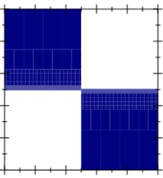
Figure 1 depicts the intermediary’s optimal product range when the product space is = [0;1]2, the distribution over it is G( ; v) = v, and the search cost distribution is

F (s) =s. The intermediary stocks the products in the shaded areas, and total industry pro…t is12:5% higher than it would be with no intermediary.26

24_{This is because Lemma 2 shows thatI(^v; )has strictly positive measure, which from the de…nition}

ofv^implies^v₂(v; v), and moreover by assumption s₂(0; s]wheres v.

25_{If we consider a discrete number of products}

f( i; vi)gi=1;:::;N, the intermediary’s problem becomes

maxqi2f0;1g

P

iqi i[F(^v) F(vi)]withv^=Piqivi=Piqi. This is a combinatorial optimization problem.

In general it is not easy to solve because there are2N _{possible stocking policies (which is very large even}

for a few dozen products). One approach is to make the problem smooth by allowing stochastic stocking policies with qi 2 [0;1], such that we can use the Lagrange method and obtain bang-bang solutions.

However the solutions for^vand are then complicated functions of the locations of individual products in the product space.

26_{The curve} ^v v

F(^v) F(v)which divides up the product space is constant when search costs are uniformly

0.0 0.2 0.4 0.6 0.8 1.0 0.0 0.2 0.4 0.6 0.8 1.0 v pi

Figure 1: Optimal product range in the simple case

Finally, we discuss the welfare impact of the intermediary in this simple case. The intermediary harms consumers because they do not enjoy any search e¢ ciencies (due to

h(m) = m) and because they have less choice (due to exclusivity). Speci…cally, consumers with s < ^v who search the intermediary buy some low-v products which they otherwise would not buy. Similarly consumers with s >v^who do not search the intermediary are unable to buy some attractive high-v products which are now only available at the inter-mediary. Nevertheless the intermediary may improve total welfare, de…ned as the sum of industry pro…t and consumer surplus. Indeed this is the case in the above example, where total welfare increases by about2:5%. Intuitively, consumers search too few manufactur-ers: they search and buy only if s < v, but from a welfare perspective they should do so whenever s < +v. Moreover amongst products with the same +v, this problem of ‘under search’is more severe for those with low-v and high- . Since the intermediary’s optimal product selection leads to an expansion in demand for these products, its presence can increase total welfare. Nevertheless the intermediary does not account for the harm it imposes on consumers and so its product selection is not socially optimal. We discuss the socially optimal product selection in the next section.

4

The General Case

We now consider the general case in which i) the intermediary can o¤er both exclusive and non-exclusive contracts, ii) the cost of searching the intermediary is h(m) s with h(m) weakly increasing, and iii) there is a limitm on the measure of products the intermediary can stock. Let qE( ; v) be an indicator function which is 1 if and only if product ( ; v) is stocked exclusively, and let qN E( ; v) be an indicator function which is 1 if and only if product ( ; v) is stocked non-exclusively. Let q( ; v) = (qE( ; v); qN E( ; v)) denote the stocking policy function, and note that q( ; v) _{2 f}(0;0);(0;1);(1;0)_g. It is again

convenient to let

q( ; v) qE( ; v) +qN E( ; v)_{2 f}0;1_g

denote whether or not product( ; v)is stocked. Henceforth whenever there is no confusion we will suppress the arguments ( ; v)in the stocking policy function.

4.1

Consumer search behavior

We …rst solve for consumers’optimal search rule given a stocking policy q. Recall from Lemma 1 that all sellers of a product charge the same price. Hence a consumer will never search both the intermediary and a manufacturer whose product is stocked there. Moreover if a consumer does consider searching a manufacturer, she will only do so if

v > s. It is also straightforward to see that the order in which a consumer visits the various manufacturers and the intermediary does not matter. Therefore a consumer who searches the intermediary and has a unit search cost s gets an expected surplus

u1(s;q) = Z qvdG h Z qdG s+ Z v>s (1 q) (v s)dG ; (10)

where the …rst two terms are surplus obtained directly from the intermediary, and the …nal term is surplus obtained by searching products not available at the intermediary. Notice that onlyq=qE+qN E matters, and not whether products are stocked exclusively or non-exclusively.

At the same time, a consumer of type s who does not search the intermediary gets expected surplus

u0(s;q) =

Z

v>s

(1 qE) (v s)dG ; (11)

because she can only buy products which are available from their manufacturers (i.e. those not stocked exclusively by the intermediary). This surplus is lower when the intermediary stocks more products exclusively (precisely, for a …xedq more products haveqE = 1). In order to ease the exposition, we suppose that a consumer searches the intermediary if and only if doing so strictly improves her payo¤ (i.e. if u1_{(s;q) > u}0_{(s;q)). The optimal}

search rule is as follows:

Lemma 3 Consumers search the intermediary if and only if s <s^, where (i) s^= 0 (nobody searches the intermediary) if R qEdG= 0 and

R

qdG h R qdG .

(ii) s > s^ (everybody searches the intermediary) if R qvdG > h R qdG s. (iii) s^₂(0; s] otherwise and is the unique strictly positive solution to

^ s= R v<s^qvdG+ R v>s^qEvdG h(R qdG) R_v>^sqN EdG : (12)

Intuitively in this general case a consumer’s decision of whether to search the interme-diary is in‡uenced by both the products it stocks (and their exclusivity) and the economy of search it generates. According to part (i) of the lemma, no consumer visits the inter-mediary when all its products are non-exclusive and it generates diseconomies of search. This is because in that case all the intermediary’s products can be acquired elsewhere at a lower search cost. On the other hand, part (ii) shows that all consumers visit the intermediary when it generates su¢ ciently strong economies of search.

Part (iii) shows that in other cases consumers follow a cut-o¤ strategy, and search the intermediary provided their search cost is su¢ ciently low. Intuitively, the advantage of shopping at the intermediary is that it stocks some exclusive products and/or has a better search technology, while the disadvantage is having to buy some low-v products. Con-sumers with lows would like to buy most products anyway and so the latter disadvantage is small.27

Finally, notice that s^in (12) degenerates to the average surplus v^de…ned in (2) if all stocked products are exclusive and h(m) =m. We use a di¤erent notation in this general case to emphasize that the threshold is now no longer the simple average surplus of the products sold at the intermediary.

4.2

Optimal product range

Given the monopoly pricing result in Lemma 1 and the consumer search rule in Lemma 3, the intermediary’s pro…t when it chooses a stocking policy qis

(q) = Z v<s^ q [F(^s) F(v)]dG+ Z v>^s qE [F(^s) F(v)]dG : (13) Firstly, the intermediary earns [F(^s) F(v)] > 0 on products with v < ^s irrespective of whether they are stocked exclusively or non-exclusively (i.e. only q = qE +qN E mat-ters). Intuitively, even under non-exclusivity the manufacturer makes zero direct sales, because consumers withs <^sbuy its product from the intermediary and consumers with

s s^ are not willing to search it. Hence the intermediary earns variable pro…t F (^s) and pays the manufacturer its outside option F (v). Secondly, the intermediary earns [F(^s) F(v)] <0 from stocking products with v >s^exclusively, and the explanation is the same as in the simple case. Lastly, the intermediary earns zero pro…t from stocking products with v > ^s non-exclusively. The reason is that when a manufacturer signs a non-exclusive contract, consumers with s <s^switch and buy its product from the inter-mediary, but consumers with s ₂ (^s; v) continue to buy direct. Hence the intermediary only needs to compensate the manufacturer by F (^s)which equals its own revenue from

27_{Notice that consumer search behavior is a¤ected only by the measure (and not the identity) of}

non-exclusive products withv >^s. This is because consumers withs <s^would buy these products anyway, so making them available at the intermediary only changes the search cost associated with buying them.

selling that product. Note that although the intermediary breaks even on these products, it may stock them in order to in‡uence consumer search behavior.

The following lemma provides a simple su¢ cient condition under which the interme-diary is guaranteed to earn strictly positive pro…t.

Lemma 4 The intermediary stocks a strictly positive measure of products and earns a strictly positive pro…t if there exists an m~ ₂(0; m) such thath( ~m) m~.

We now characterize the optimal product selection when the intermediary can prof-itably exist with s >^ 0. The intermediary wishes to maximize its pro…t from equation (13) given the space limitm 1, where^swas de…ned earlier in Lemma 3. Whens^₂(0; s] we know that ^s satis…es equation (12), which we can rewrite as

Z v<^s qvdG+ Z v>^s (qEv+qN Es^)dG h(m)^s = 0 ; (14) where m denotes the measure of products stocked by the intermediary and satis…es

m=

Z

qdG : (15)

The stocking space constraint can be written as

m m : (16)

It is again convenient to solve the intermediary’s problem using the Lagrangian method, treating (14)-(16) as constraints. Let , and be their respective Lagrange multipliers (and note that = 0 if s > s^ because in that case the constraint (14) does not apply). After some manipulations we can write the (Kuhn-Tucker) Lagrange function as

L = Z v<s^ q_f [F (^s) F (v)] + v _gdG + Z v>^sf qE[ [F (^s) F (v)] + v ] +qN E( ^s )gdG ^ sh(m) + m+ (m m) : (17)

It is again useful to decompose the Lagrange function into direct and indirect e¤ects of stocking product ( ; v). The direct e¤ect is the pro…t generated by the product: recall from earlier that it is zero if the product is non-exclusive andv >s^, and otherwise equals [F(^s) F (v)]. The indirect e¤ect is the change in pro…ts from other products due to changes in consumer search behavior: it equals s^ if the product is non-exclusive and

v >s^, and otherwise is v . Since the integrands are again linear in stocking variables, we have the following characterization of the optimal product selection:

Proposition 2 Suppose the intermediary earns a strictly positive pro…t (e.g. the condi-tion in Lemma 4 is satis…ed). The optimal product seleccondi-tion is as follows (with s >^ 0,

0 and 0 de…ned in the proof ):

(i) Products with v <s^are stocked if and only if

v

F(^s) F(v) ; (18)

and it does not matter whether these products are exclusive or not. (ii) Products with v >s^are stocked exclusively if and only if

max_f s;^ _g v

F(^s) F(v) : (19)

Of the other products with v > s^: if ^s > all of them are stocked non-exclusively, if ^

s = some of them are stocked non-exclusively, and if s <^ none of them are stocked. As in the simple case, the intermediary stocks some high-v and low- products ex-clusively to attract consumers, and some low-v and high- products to generate pro…ts. An important di¤erence is that now the intermediary may also stock high-v and high-products non-exclusively.28 _{Whether or not that happens depends on the sign of the}

in-direct e¤ect s^ .29 _{In general it appears hard to …nd primitive conditions for the sign}

of s^ , but we have the following useful observation:

Corollary 1 If the space constraint is not binding (m < m) in the optimal product se-lection, then = sh^ 0(m). Hence in the region of v > s^, all products are stocked if

h0(m)<1, but only low- products are stocked (exclusively) if h0(m)>1.

Corollary 1 shows that in an interesting special case of the model, when the interme-diary generates (marginal) diseconomies of search its optimal product selection has two negatively correlated regions in the ( ; v) space (as in the simple case).30

According to Proposition 2 the intermediary is indi¤erent about stocking products with v < ^s exclusively or non-exclusively. (This is because exclusivity has no e¤ect on either the direct pro…t in equation (13) or on consumer search behavior in Lemma 3). One way to break this indi¤erence is to introduce some small-demand consumers who never

28_{Another subtler di¤erence is that unlike in the simple case it is possible that^s < v(whenv >0and}

diseconomies of search are strong) ors > v^ (when economies of search are strong). In these cases only one part of Proposition 2 is relevant.

29_{If ^s = 0the intermediary is indi¤erent about which of these non-exclusive products to stock}

(and the equation s^ = 0pins down their measure). In this case the optimal selection is not unique.

30_{These two regions are also disconnected, because given h}0_{(m)>1, asv !^sthe thresholds in (18)}

and (19) tend respectively to ₁and ₁. Intuitively products withv s^generate only a small direct pro…t or loss, so their negative e¤ect on consumers’incentives to search the intermediary dominates.

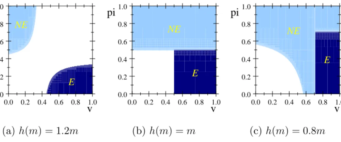
visit the intermediary. In that case the intermediary strictly prefers to stock products with v <s^non-exclusively, because it reduces the compensation paid to manufacturers. Therefore in subsequent analysis we interpret products withv <^sas being non-exclusive. We now illustrate the optimal product selection using some examples. First, we il-lustrate how the intermediary’s search technology a¤ects its product selection. Figure 2 considers an example with F(s) = s and G( ; v) = v and no space constraint (i.e.

m= 1).31 _{The search technology is h(m) = 1:2m in part (a), h(m) =m in part (b), and} h(m) = 0:8min part (c). Consistent with Corollary 1, whenh(m) = 1:2monly the low-products with v >s^are stocked (exclusively), whereas when h(m) = 0:8m all products with v >s^are stocked. (When h(m) =m the intermediary is indi¤erent about stocking each product in [0:5;1]2 non-exclusively. The …gure depicts the case where the interme-diary stocks all these products.) Comparing across the three cases, as the intermeinterme-diary’s search technology becomes more e¢ cient it stocks more products (m increases from 0:29 to 0:75 and then to0:76) but a smaller proportion of them are exclusive (the percentage decreases from 50% to 33% and then to 27%). Intuitively, the intermediary relies less on exclusive products to attract consumers when it already helps to reduce their search costs. NE E 0.0 0.2 0.4 0.6 0.8 1.0 0.0 0.2 0.4 0.6 0.8 1.0 v pi (a) h(m) = 1:2m E NE 0.0 0.2 0.4 0.6 0.8 1.0 0.0 0.2 0.4 0.6 0.8 1.0 v pi (b) h(m) =m E NE 0.0 0.2 0.4 0.6 0.8 1.0 0.0 0.2 0.4 0.6 0.8 1.0 v pi (c) h(m) = 0:8m

Figure 2: Optimal product range and search technology

Second, we illustrate how the space limit m a¤ects product selection. Figure 3 con-siders an example with F(s) = s and G( ; v) = v (as above), and also h(m) = 0:4 such that the cost of visiting the intermediary is independent of its size. In this exam-ple marginal economies of search are so strong that the intermediary always uses all its stocking space. In part (a) m = 0:3 and the optimal solution has s^ < 0, hence the intermediary stocks products in two negatively correlated and disconnected regions.

31_{This example withh(m) =a+bmcan be fully solved. A su¢ cient condition for the intermediary to}

In part (b) m = 0:46 and the optimal solution has ^s = 0, hence the intermediary stocks some but not all of the products in the top-right corner non-exclusively. (As dis-cussed in footnote 29, when s^ = 0 the optimal solution in the top-right corner is not unique. In particular, only the measure of products that are stocked non-exclusively can be determined. Conditional on stocking the correct measure of products, the inter-mediary is indi¤erent over exactly which products in the top-right corner to stock. The …gure depicts the case where the intermediary stocks those with the highest v.) In part (c) m = 0:5 and the optimal solution has s^ > 0, hence all products with v > ^s

are stocked.32 _{Comparing across the three cases, as the intermediary becomes able to}

stock more products, it attracts more consumers (^sincreases from0:32to0:7and then to 0:81) but stocks proportionately fewer exclusive products (the percentage decreases from 50% to45:6% and then to30:5%), while sales outside the intermediary fall (from0:37to 0:22, and then to 0:175). Notice that qualitatively the e¤ect of a better search technology (Figure 2) and larger space limit (Figure 3) are the same.

NE E 0.0 0.2 0.4 0.6 0.8 1.0 0.0 0.2 0.4 0.6 0.8 1.0 v pi (a)m= 0:3 NE E 0.0 0.2 0.4 0.6 0.8 1.0 0.0 0.2 0.4 0.6 0.8 1.0 v pi (b)m = 0:46 NE E 0.0 0.2 0.4 0.6 0.8 1.0 0.0 0.2 0.4 0.6 0.8 1.0 v pi (c)m= 0:5 Figure 3: Optimal product range and stocking space constraint

4.3

Socially optimal product range

We now brie‡y study the socially optimal product range. Suppose a social planner wishes to maximize total welfare, and it can choose the stocking policyqbut has no direct control over …rm pricing or how consumers search. This problem can be solved in a similar way to the intermediary’s. We therefore report the main result here and relegate the details to the online appendix.

32_{The product selection is similar to Figure 3(a) formbelow around0:454, similar to Figure 3(b) for}

m between around 0:454 and 0:463, and similar to Figure 3(c) for m between around 0:463 and 0:65. Whenmexceeds around0:65the intermediary’s size and strong economies of search enable it to attract all consumers, none of its products are exclusive, and only low-v and low- manufacturers make direct sales.

Proposition 3 A su¢ cient condition for the socially optimal stocking policy to have

m >0is thath( ~m) m~ for somem~ ₂(0; m). The socially optimal policy is characterized as follows (with s >^ 0, 0 and 0 de…ned in the proof ):

(i) Products with v <s^are stocked if and only if

+v v

Rv

0 sdF(s)

F(^s) F(v) ; (20)

and it does not matter whether they are exclusive or not. (ii) Products with v >s^are stocked exclusively if and only if

+v maxf ; s^+ R^s 0 sdF(s)g v Rv 0 sdF(s) F(^s) F(v) : (21)

Of the other products with v > s^: if s^+R₀s^sdF(s) > all of them are stocked non-exclusively, if s^+R₀^ssdF(s) = some of them are stocked non-exclusively, and if s^+

R^s

0 sdF(s)< none of them are stocked.

The welfare-optimal stocking policy is qualitatively the same as the one used by the intermediary. Firstly, exclusive products withv >s^are again chosen to have low , and products with v < s^are chosen to have high . Intuitively this is because, as we noted earlier, consumers do not take into account sellers’pro…t, and therefore search (and buy) too little from a welfare perspective. Demand for a product with v >s^is further reduced when it is sold exclusively by the intermediary, but conversely demand for a product with

v < s^ is increased when it is sold by the intermediary. Choosing the former products to have low minimizes the additional welfare loss, and choosing the latter to have a high maximizes the welfare gains. Secondly, and mirroring Corollary 1 from earlier, we can show that when the stocking constraint is slack at the optimum all products with

v > ^s are stocked if h0(m) < 1, but only those with low are stocked (exclusively) if

h0_{(m) > 1. Intuitively, when the intermediary adds some non-exclusive products with}

v > ^s all the consumers with s < s^ will switch their purchases of those products away from manufacturers towards the intermediary, and their total search cost falls ifh0_(m)<1

but increases if h0_(m)>1.

We would now like to compare the stocking policies chosen by the intermediary and social planner. Unfortunately this is hard to do analytically, because in general (^s; ; ) di¤er across the two solutions and are determined by a complex system of equations. Intuitively though, one would expect the social planner to stock fewer high-v products exclusively since this harms consumers that do not search the intermediary. Similarly, if economies of search are not too strong, one would expect the social planner to stock fewer low-v products because consumers who search the intermediary end up buying them even though they provide little surplus. We con…rm this intuition using our running

example with G( ; v) = v and F(s) =s. Suppose there is no stocking space constraint. Figure 4(a) plots the socially optimal product range for the caseh(m) = 1:2m. Since the intermediary has diseconomies of search, this product range is now much smaller than (and is a subset of) that in Figure 2(a). Figure 4(b) plots the socially optimal product range for the case h(m) = m. It turns out that in this case (^s; ; )are the same as in Figure 2(b). The social planner’s product range is also a strict subset of the intermediary’s, and it stocks fewer products exclusively. Figure 4(c) plots the socially optimal product range for the case h(m) = 0:8m. Here (^s; ; ) di¤er from Figure 2(c), and the social planner’s selection is not a subset of the intermediary’s. Nevertheless the intermediary again stocks fewer products overall and also fewer products exclusively.

E NE 0.0 0.2 0.4 0.6 0.8 1.0 0.0 0.2 0.4 0.6 0.8 1.0 v pi (a) h(m) = 1:2m E NE 0.0 0.2 0.4 0.6 0.8 1.0 0.0 0.2 0.4 0.6 0.8 1.0 v pi (b) h(m) =m E NE 0.0 0.2 0.4 0.6 0.8 1.0 0.0 0.2 0.4 0.6 0.8 1.0 v pi (c) h(m) = 0:8m

Figure 4: Socially optimal product range

Finally, even though our results suggest that the intermediary stocks too many ex-clusive products, a complete ban on exclusivity is not necessarily welfare enhancing. For example in the simple case withh(m) =m, a ban on exclusivity prevents the intermediary from existing and so strictly reduces total welfare.

5

Two Applications

We now apply our framework to examine the optimal design of a shopping mall (which acts as a platform and does not directly set prices) and the e¤ect of DTC sales on retail markets. Here in each application we lay out various theoretical predictions and then document relevant empirical evidence in the following section of the paper.

5.1

Shopping malls

Suppose there is a unit mass of sellers each of which can either join a shopping mall and/or set up its own independent shop in the same area. The mall can host up to a measure m

of sellers, and charges each of them a …xed fee. Consumers pay n s to search a measure

n of independent shops and h(m) s to search a mall which contains a measure m of shops. The timing is exactly as in Section 4 except that now the mall is a platform and therefore individual sellers set prices.

Our earlier analysis applies straightforwardly. Firstly, it is easy to see that seller i

should charge pm

i wherever it sells its product. (We do not even need Lemma 1.) Hence our( ; v)representation remains valid. Secondly, consumers search the mall if and only if

s <s^where^swas de…ned earlier in Lemma 3. Thirdly, sales of a product( ; v)at the mall generate a gross pro…t of F (^s). Therefore a seller withv <s^will pay [F(^s) F (v)]to join the mall, whilst a seller withv >s^is willing to join the mall for free if it also maintains an independent store elsewhere, but must be paid [F (v) F (^s)]to exclusively join the mall. Consequently the mall owner’s pro…t is the same as in equation (13).

The optimal mix of stores within the mall is exactly as in Proposition 2. Using some terminology from existing literature, we can interpret sellers withv >s^who are exclusive to the mall as ‘anchor stores’. According to our model, the mall owner should subsidize anchor stores to encourage them to join. This is worthwhile because their presence attracts more consumers (i.e. increases s^), which allows the mall to charge a higher fee to other ‘non-anchor’stores.

5.2

Direct-to-consumer sales

We argued in the introduction that it has become increasingly easy for manufacturers to sell direct to consumers. Our framework can be extended to look at the consequences of easier DTC sales. To this end consider the general case from Section 4, but now index products by ( ; v; ) where > 0 represents how easy it is for consumers to buy direct from the product’s manufacturer. Speci…cally, a consumer with unit search cost s, if she visits a measure n of manufacturers with DTC index , incurs a total search costn s. Importantly we assume that can di¤er across products (so that direct sales are easier for products with a lower ), and we say that all products with a common belong to the same ‘sector’. We letG( ; v; )be the joint distribution over the product space, and[ ; ] be the support of . We also assume that conditional on the ( ; v) space is compact and convex, and v s to avoid corner solutions.

We start by characterizing the intermediary’s optimal product selection. We then consider what happens as DTC sales become easier in certain sectors. All the omitted details in this section can be found in the online appendix.

5.2.1 Optimal stocking policy

An important di¤erence with the baseline model is that if the manufacturer of a product ( ; v; ) only sells direct to consumers, it sells to all consumers for whom v > s. Hence

the manufacturer’s outside option is F(v= ). As one would expect this outside option is higher when is lower i.e. when direct sales are easier. This already suggests that the intermediary will have less incentive to carry products which are easier to sell direct.

Analysis of consumer search and intermediary pro…t closely follows that from Section 4. Consumers visit the intermediary if and only if their search cost is below a threshold ^

s which is de…ned in a similar way to in Lemma 3 from earlier. The intermediary earns a positive pro…t on products with v < ^s and exclusivity does not matter; for products with v > ^s it breaks even when stocking non-exclusively, and makes negative pro…t when stocking exclusively.33 _{We then obtain the following characterization of the optimal}

stocking policy:

Proposition 4 The optimal stocking policy is characterized as follows (withs >^ 0, 0 and 0 de…ned in the proof ):

(i) Products with v < ^s are stocked if and only if

v

F(^s) F(v) ; (22)

and it does not matter whether these products are exclusive or not. (ii) Products with v > s^are stocked exclusively if and only if

max_f s;^ _g v

F(^s) F(v) : (23)

Of the other products with v > s^: if s^ > 0 they are stocked non-exclusively, if ^

s = some of them are stocked non-exclusively, and if s^ <0 none of them are stocked.

Given a particular the conditions for whether and how a product is stocked are similar to those from the general case. Using Proposition 4 we can derive two implications for how the stocking policy di¤ers across sectors. The …rst is:

Corollary 2 Consider products with the same ( ; v). If the intermediary stocks (exclu-sively or non-exclu(exclu-sively) one in sector 0, then it also stocks all those in sectors > 0.

Corollary 2 further implies that in the special case where the distribution of is inde-pendent of( ; v)then more products are stocked by the intermediary in higher- sectors. One reason (as alluded to above) is that manufacturers with higher- products have a worse outside option and so are cheaper for the intermediary to contract with. Another reason is that the indirect bene…t to the intermediary of stocking higher- products is also higher, because by stocking these products the intermediary saves consumers who visit it more search costs. A second implication is the following:

33_{Closely following Lemma 4 we can also show that a su¢ cient condition for the intermediary to}

Corollary 3 Supposem < m at the optimum and consider products with s^₂(v; v). (i) Among those with < h0(m) none are stocked forv in a neighborhood of s^, and none withv > ^sare stocked non-exclusively. That is, in sectors where DTC sales are relatively easy, the intermediary only stocks products in two disconnected and negatively-correlated regions.

(ii) Among those with > h0_{(m) all are stocked for v in a neighborhood of s^, and all}

with v > ^s are stocked. That is, in sectors where DTC sales are relatively hard, the intermediary’s product range is a connected set which includes all high-v products.

Corollary 3 suggests that in an interesting special case of the model, product selection is more ‘polarized’ in sectors where DTC is easier. Intuitively, the intermediary …nds it relatively expensive to stock products with < h0_{(m) and also generates search}

dis-economies on them. Hence it stocks exclusively a small measure of high-v and low-products which are very successful in attracting consumers, and stocks a small measure of low-v and high- products which are particularly pro…table. On the other hand, the intermediary …nds it relatively cheap to stock products with > h0_{(m)and also generates}

search economies on them. Hence the optimal product selection is very di¤erent.34

5.2.2 Changes in the ease of DTC sales

We now consider the e¤ect of improvements in technology which make DTC sales easier. Formally, DTC sales become easier when for each sector the DTC sales cost index for product ( ; v; ) decreases to ( ; ; v) , with a strict inequality for a positive measure of sectors.35 _{We assume throughout that the cost of visiting the intermediary}

is unchanged, which is plausible when the intermediary is an o- ine retailer such as a supermarket or department store.

We begin with the following straightforward result:

Corollary 4 When DTC sales become easier, manufacturer pro…t increases while the

intermediary’s pro…t decreases.

Manufacturers clearly bene…t since they always earn their outside option F (v= ), and this strictly increases for any manufacturer whose product becomes strictly easier

34_{In the limit case where ! 1for all products (and so DTC sales are impossible), the intermediary}

stocks products with ( v)=F(^s), i.e. those with high and highv. Intuitively the intermediary does not need to compensate manufacturers beyond their marginal cost, and so carries products with highv to attract consumers and high to maximize variable pro…ts.

35_{Here we implicitly assume that DTC sales become easier for exogenous reasons e.g. due to the}

development of online marketplaces. In practice manufacturers can also invest in direct channels. Fixing the investment cost, and under some regularity conditions, manufacturers with high-vand high- products are more likely to invest i.e. ( ; ; v)falls more for those products.

to sell direct. On the other hand the intermediary is made worse o¤. It is easy to see that if the intermediary does not change its stocking policy it becomes worse o¤, both because it has to compensate manufacturers more, and because easier DTC sales leads to a reduction in the measure of consumers that use the intermediary; Corollary 4 then shows that the intermediary is still worse o¤ even after it adjusts its stocking policy.

We now discuss in more detail how the intermediary should adjust its stocking policy as DTC sales become easier. Unfortunately in general it is impossible to provide analytical results. Therefore we use an example to illustrate the main insight. Suppose that m = 1, h(m) = m, ( ; v) is on [0;1]2 _{uniformly, F(s) = s=2 with support [0;2],}36 _and

has a binary distribution, independent of ( ; v), with Pr( = 1=2) = z and Pr( = 3=2) = 1 z, where z ₂ [0;1]. We vary the proportion z of products for which DTC sales are easy. As z increases more products fall in the low- sector, and therefore the intermediary carries fewer products as described in Figure 5(a), but a higher proportion of them are exclusive as described in Figure 5(b). Intuitively, when it becomes easier to sell certain products direct, their manufacturers must be compensated more and so it is less pro…table for the intermediary to still carry them. At the same time, however, easier direct sales reduce consumers’need to search the intermediary, and so the intermediary relies more on product exclusivity to remain attractive. Figure 5(c) then plots the total measure of co