DOI 10.1007/s10878-007-9114-0
Single machine batch scheduling with release times
Beat Gfeller·Leon Peeters·Birgitta Weber· Peter Widmayer
Published online: 22 November 2007
© Springer Science+Business Media, LLC 2007
Abstract Motivated by a high-throughput logging system, we investigate the sin-gle machine scheduling problem with batching, where jobs have release times and processing times, and batches require a setup time. Our objective is to minimize the total flow time, in the online setting. For the online problem where all jobs have iden-tical processing times, we propose a 2-competitive algorithm and we prove a cor-responding lower bound. Moreover, we show that if jobs with arbitrary processing times can be processed in any order, any online algorithm has a linear competitive ratio in the worst case.
Keywords Batch scheduling·Online algorithms·Competitive analysis
A preliminary version of a part of this paper was presented at the 31st International Symposium on Mathematical Foundations of Computer Science (MFCS 2006). We gratefully acknowledge reviewers’ comments that helped to improve the presentation of this work.
Supported by the Swiss SBF under contract no. C05.0047 within COST-295 (DYNAMO) of the European Union.
Research carried out while B. Weber was affiliated with the Institute of Theoretical Computer Science, ETH Zurich.
B. Gfeller (
)·L. Peeters·B. Weber·P. WidmayerInstitute of Theoretical Computer Science, ETH Zurich, Zurich, Switzerland e-mail:[email protected] L. Peeters e-mail:[email protected] B. Weber e-mail:[email protected] P. Widmayer e-mail:[email protected]
1 Introduction
The study in this paper is motivated by the real world problem of saving a log of actions in a high throughput environment. Many actions are to be carried out in rapid succession, and in case of a system failure the log can identify which actions have been carried out before the failure and which have not. Keeping such a log can be existential for a business, for example when logging the trading data in a stock bro-kerage company.
Logging takes place on disk and is carried out by a storage system that accepts write requests. When a process wants its data to be logged, it sends a log request with the log data to the storage system and waits for the acknowledgement that the writing of the log data has been completed. For the log requests that arrive over time at the storage system, there is only one decision the system is free to make: What subset of the requested, but not yet written log data should be written to disk in a single large write operation to make the whole system as efficient as possible? After the chosen large write operation is complete, the system instantaneously sends acknowledgements to all processes whose requests have been satisfied.
The difficulty in the above question comes from the fact that log data come in all sizes (number of bits or blocks to be stored), that writing several log data in a sin-gle shot is faster than writing each of them individually (due to the disk hardware constraints), and that a process requesting a write has to wait for the acknowledge-ment (of the completion of the large write operation) before it can continue. Based on an experimental evaluation of writing data to disk, we assume the writing time for a number of data blocks to be linear in that number, plus an additive constant (for the disk write setup time). Our objective is to minimize the sum over all requests of the times between the request’s arrival and its acknowledgement. We ignore the details of a failure and its recovery here, and are not worrying about (the potential loss of) unsatisfied write requests.
1.1 Single machine scheduling with batching
Viewing the storage system as a machine, the log requests as jobs, and the write operations as batches, this problem falls into the realm of scheduling with batching (see the overview by Potts and Kovalyov2000). More precisely, in the usual batch scheduling taxonomy of Potts and Kovalyov (2000) we deal with a family scheduling
problem with batching on a single machine where all the jobs belong to the same
family. The machine processes the jobs consecutively, since the log data are stored consecutively in time on the disk (as opposed to simultaneously), and each batch of jobs requires a constant (disk write) setup time. As all log requests in a single write are simultaneously acknowledged at the write completion time, the machine operates with batch availability, meaning that each job in the batch completes only when the full batch is completed.
In more formal terms, we model the storage system as a single machine, and the log requests as a set of jobsJ= {1, . . . , n}. The arrival times of the log requests at
the storage system then correspond to job release timesrj, j ∈ {1, . . . , n}. Further,
of the log request. The grouping of the log requests into write operations is modeled by the batching of the jobs into a partitionσ= {σ1, . . . , σk}of the jobs {1, . . . , n},
whereσurepresents the jobs in theu-th batch,kis the total number of batches, and
we refer to|σu|as the size of batchu, defined as the number of jobs inσu. Unless
stated otherwise, we assume that the batch size is not limited. We denote the starting time of batchσubyTu, withrj≤Tufor allj ∈σu. Starting atTu, the batch requires
a constant setup times for preparing the disk write, and further a total processing timej∈σupj, for writing the logs on the disk. Thus, each batchσu requires a total
batch processing timePu=s+
j∈σupj. The consecutive execution of batches on
the single machine translates intoTu+Pu≤Tu+1foru=1, . . . , k−1. Because of batch availability, each jobj∈σucompletes at timeCj=Tu+Pu, and takes a flow timeFj =Cj −rj to be processed. This job flow time basically consists of two components: first a waiting timeTu−rj≥0 that the job waits before batchσustarts, followed by the batch processing timePu. Finally, as mentioned above, our objective is to minimize the total job flow timeF=nj=1Fj.
We refer to this scheduling problem as the BATCHFLOW problem. In the stan-dard scheduling classification scheme, the BATCHFLOWproblem is written as 1|rj,
sf =s, F =1|Fj, where the partsf =s, F =1 refers to the fact that each job family has a fixed setup time and all jobs belong to the same family (see Potts and Kovalyov2000). As special cases, we consider the problem variants with
identi-cal processing timespj =p, and with a fixed job sequence, where jobs are to be processed in release order.
1.2 Online algorithms for a single machine with batching
In the online version of the BATCHFLOWproblem, jobs are released over time, and any algorithm can base its batching decisions at a given time instant only on the jobs that have been released so far. We study the online problem under the non-preemptive
clairvoyant setting: No information about a job is known until it is released, but once
a jobj has been released, both its release timerj(that is, arrival time) and processing timepj are known. A batch that has started processing cannot be stopped before completion.
In this paper we consider deterministic online algorithms. Without loss of gener-ality, we assume that these algorithms have a particular structure, as described in the following.
From the problem definition it follows that no online algorithm can start a new batch as long as the machine is busy. Furthermore, any online algorithm needs to revise a decision only when new information becomes available, that is, when a new job is released. Therefore, we consider online algorithms that only take a decision at the completion time of a batchσu, or when a new jobj is released and the machine
is idle. We refer to these two events as triggering events. In either case, the algorithm bases its decision on the jobs{1, . . . , j}that have been released so far, and on the batchesσ1, . . . , σu created so far. Note that the setP of currently pending jobs can
be deduced from this information.
In case of a triggering event, an online algorithmAtakes the following two deci-sions. First, it tentatively chooses the next batchσAto be executed on the machine.
However, it does not execute the batchσAimmediately. Rather, the algorithm’s sec-ond decision defines a delay timeΔA by which it delays the execution ofσA, and waits for a triggering event to occur in the meantime. IfΔAtime has elapsed, and no triggering event has happened, then the algorithm starts the batchσAon the machine (by definition, the machine is idle in this case). If, however, a triggering event occurs during the delay time, then the algorithm newly choosesσAandΔA. Thus, an online algorithmAis completely specified by how it choosesσAandΔA.
To evaluate different online algorithms for the online BATCHFLOWproblem, we use competitive analysis: For a given problem instanceI, letFOPT(I )be the total flow
time of an optimal solution, andFA(I )the total flow time of the solution obtained from some online algorithmA. We are interested in the strict competitive ratio of online algorithmA, defined as supI FFA(I )
OPT(I ). The online algorithmAisc-competitive
if there is a constantαsuch that for all instancesI,FA(I )≤c·FOPT(I )+α.When
this condition holds also forα=0, we say thatAis strictlyc-competitive.
1.3 Related work
Sincej∈Jrjis a constant that we cannot influence, the offline version of our
prob-lem is equivalent to the probprob-lem 1|rj, sf =s, F =1|Cj. The related problem 1|sf =s, F =1|
Cj, without release times but with individual processing times,
was first considered by Coffman et al. (1990). They solve this problem inO(nlogn)
time, first sorting the jobs by processing time, and then using an O(n) dynamic programming algorithm. Albers and Brucker (1993) extend that solution to solve 1|sf =s, F=1|wjCj for a fixed job sequence inO(n)time, and show that the unrestricted problem 1|sf =s, F=1|
wjCjis unary NP-hard. Webster and Baker
(1995) describe a dynamic program with running timeO(n3)for the so-called batch
processing model, where each batch has the same size-independent processing time,
but the batch size is limited.
More recently, Cheng and Kovalyov (2001) describe complexity results for various related problems and objectives, also considering due dates, but not release times. They consider the bounded model, where the size of a batch1can be at mostB, as well as the unbounded model.
The objective of minimizing the total completion time (weighted or unweighted) has been considered also in the so-called burn-in model (see Lee et al.1992), where the processing time of a batch is equal to the maximum processing time among all jobs in the batch. For this model, Poon and Yu (2004) present two algorithms for 1|sf =s, F =1, B|Cj with batch size boundB, with running timesO(n6B)and
nO(√n). Furthermore, Deng et al. (2004) consider 1|sf =s, F =1|
wjCj in the
burn-in model with unbounded batch size. They show NP-hardness of that problem, and give a polynomial time approximation scheme.
Concerning the online setting, most previous work focuses on the burn-in model. An exception is Divakaran and Saks (2001), who consider the problem 1|rj, sf|maxFj with sequence-independent setup times and several job families
un-der job availability (i.e. the processing of each job completes as soon as its processing 1This bound is also called capacity by some authors.
time has elapsed). They present anO(1)-competitive online algorithm for that prob-lem. For the burn-in model, Chen et al. (2004) consider the problem 1|rj|wjCj, and present a 10/3-competitive online algorithm for unbounded batch size, as well as a 4+ε-competitive online algorithm for bounded batch size.
The online problem 1|rj|Cmaxof minimizing the makespan in the burn-in model has been considered in several studies. Independently, Deng et al. (2003) and Zhang et al. (2001) gave a(√5+1)/2 lower bound for the competitive ratio, and both gave the same online algorithm for the unbounded batch size model which matches the lower bound. Poon and Yu (2005a) present a different online algorithm with the same competitive ratio, and describe a parameterized online algorithm which contains their own and the previous solution as special cases. Poon and Yu (2005b) give a class of 2-competitive online algorithms for bounded batch size, and a 7/4-competitive algorithm for batch size limitB=2.
Bein et al. (2004) propose optimally competitive online algorithms for the list
batching problem. As in the BATCHFLOWproblem, the goal is to minimize the total flow time of jobs. However there are no release times, or equivalently, all jobs are released at time zero. Still, the algorithm learns the jobs one after the other, and each time has to decide whether to include this job as the last in the current batch and start processing the batch, or to keep the batch open for later jobs.
1.4 Contribution and outline of the paper
To the best of our knowledge, we are the first to consider release times with the ob-jective of minimizing the total flow timeFj under batch availability. We study
this problem in an online setting, call it online BATCHFLOWproblem, and introduce the GREEDYonline algorithm in Sect.2.1. For the special case of identical process-ing timesp, we show that GREEDYis strictly 2-competitive, using the fact that its makespan is optimal up to an additive constant. In Sect.2.3, we present two lower bounds, 1+ 1
1+maxmin(p,s)(p,s) and 1+ 1
1+2ps for this problem variant, and hence show that GREEDYis not far from optimal for this variant.
For the general online BATCHFLOWproblem, we then give an n2−εlower bound for the competitive ratio, and show that any online algorithm which avoids unneces-sary idle time, including GREEDY, is strictlyn-competitive, which matches the order of the lower bound.
2 The online BATCHFLOWproblem
We first analyze the online BATCHFLOWproblem for jobs with identical processing timespj=p. For this case, we present a 2-competitive greedy algorithm in Sect.2.1, and derive two lower bounds in terms ofpandsfor any online algorithm in Sect.2.3. Next, Sect.2.4discusses bounds for any online algorithm for the case of general processing times.
2.1 The GREEDYbatching algorithm for identical processing times
In this section, we consider the restricted case where all jobs have identical process-ing timespj=p. This case is relevant in applications such as ours, where records of
fixed length are to be logged. Note that the reordering of jobs with identical process-ing times is never beneficial, so it is irrelevant whether the fixed job sequence restric-tion is present or not, and we assume in the following that jobs are never reordered.
We now define the GREEDYalgorithm, which always starts a batch consisting of all currently pending jobs as soon as the machine becomes idle.
Algorithm 1 GREEDY
Whenever the machine becomes idle:
SetΔA=0 (start the next batch immediately) ChooseσA=the set of currently pending jobs
First, we focus on the makespan of GREEDY. Let us first understand how the struc-ture of the GREEDYsolution relates to alternative solutions that use fewer batches. To that end, we consider GREEDY’s solution to a given instance and compare it to some other solution for the same instance, denoted by ANY. By definition, each of these two solutions consists of a sequence of consecutive batches. We require the following lemma, which is illustrated in Fig.1.
Lemma 1 Consider a sequenceσa, . . . , σbofu GREEDYbatches, and a sequence
σc, . . . , σd ofvANYbatches, such that the ANYsequence contains all the jobs in the
GREEDYsequence (in the same order), and possibly additional jobs. Ifu≥v+1,
then there exists a batchσ∗ among ANY’s batches that contains both at least one entire GREEDYbatch, and at least one following jobj∗from the next GREEDYbatch.
Proof Instead of proving the lemma directly, we prove the following equivalent
state-ment: Assuming that no batch amongσc, . . . , σd fully contains a GREEDYbatch plus a following job, it holds thatu≤v.
We show that claim by induction overu. Foru=1 the claim is trivially true. Suppose that foru≥2, the claim holds for 1, . . . , u−1. By our assumption, the first ANYbatchσccan at most containσaentirely, but no following jobs. Thus, the jobs
inσa+1, . . . , σbmust be covered byσc+1, . . . , σd. These two sequences have lengths u−1 andv−1, respectively, so by the induction hypothesis, we have 1+u−1≤
1+v−1, thusu≤v.
The following lemma shows that if GREEDYneeds timet to finish a set of batches {σ1, . . . , σu}, then no other algorithm can complete the same jobs before timet−s.
Thus, GREEDYis 1-competitive for minimizing the makespan, with an additive con-stantα=s.
Lemma 2 For a given problem instance of the online BATCHFLOW problem with identical processing times, letσ =σ1, . . . , σk with batch starting timesT1, . . . , Tk
be the GREEDY solution, and letσ=σ1, . . . , σm withT1, . . . , Tm be some other solution ANYfor the same instance. For any batchσu∈σ completing at timet, it
holds that any batchσv∈σsatisfying the condition
v i=1 |σi| ≥ u i=1 |σi| (1) completes at timet≥t−s.
Proof For a given batchσu∈σ consider the first batchσv∈σfor which (1) holds.
Such a batch exists becausemi=1|σi| =nand of course
u
i=1|σi| ≤n (note that
u
i=1|σi| =nholds only if σu is the last GREEDY batch, i.e.,u=k). We assume that the GREEDYbatchesσ1, . . . , σuare executed without any idle time in between.
Indeed, if such an idle time occurs, GREEDYmust have processed all jobs which have been released so far, and the idle time ends exactly at the release time of the next job. Of course, ANYcannot start processing this job earlier than GREEDYdoes. Hence, ignoring all jobs before such an idle time can only affect the comparison in favor of ANY.
First, we consider the caseu≥v+1, where GREEDYuses at least one batch more than ANY. Apply Lemma1toσ1, . . . , σuandσ1, . . . , σv, and letσ∗ be the last ANY
batch containing a full GREEDYbatch followed by at least one job. Chooseσ∗such that it is the last full GREEDYbatch whose jobs are contained inσ∗ that is followed by some jobj∗inσ∗. Whenj∗ is released, GREEDYhas already started processing batchσ∗ (or has even finished), because otherwisej∗ would be part of σ∗. On the other hand, ANYcannot start processing batchσ∗ beforej∗is released. So, it must hold thatTσ∗≤Tσ∗. Letσ∗∗be the GREEDYbatch followingσ∗. Note that Lemma1
(in contraposition) can be applied also to the sequencesσ∗∗, . . . , σu andσ∗, . . . , σv. Thus, since in these two sequences no ANYbatch contains an entire GREEDYbatch followed by another job, we have|{σ∗∗, . . . , σu}| ≤ |{σ∗, . . . , σv}|. Definingzas the
number of batches in{σ∗, . . . , σu}, andzas the number of batches in{σ∗, . . . , σv}, it
holdsz≤z+1. Putting all of the above together, we obtain:
t−t≤Tσ∗+p·(|σ∗| + · · · + |σu|)+zs−Tσ∗−p·(|σ∗| + · · · + |σv|)−zs≤s.
Finally, we consider the remaining caseu≤v. Since GREEDYhas no idle time, it starts the first batch atT1, which is when the first job is released. Note that ANY cannot start a batch before this time, henceT1≥T1. GREEDYcompletesσuexactly at timet=T1+p·
u
i=1|σi|+us. ANYfinishesσvat timet≥T1+p· v
i=1|σi|+vs
or later. So, using condition (1), we obtain thatt−t≥(v−u)s, proving the theorem for anyu≤v+1, and foru≤vin particular.
Corollary 3 The GREEDY online algorithm always computes a solution with makespan at mostslarger than the minimum makespan.
From this corollary, we obtain the following lemma.
Lemma 4 In the online BATCHFLOWproblem with identical processing times, con-sider any batchσuof the GREEDYsolution, with starting timeTu. Letσbe the first
batch of the optimal solution OPTthat contains some job inσu. The earliest time that
OPTcan finish processing themjobs inσu∩σisTu+mp.
Proof Observe that, if we deleted all jobs inσu\σfrom the problem instance, then
GREEDYwould start processing exactly themjobs inσu∩σin one batch at timeTu,
and finish atTu+mp+s. Now, if OPTwere to finish thesemjobs beforeTu+mp,
then there would exist a solution with makespan more thanssmaller than GREEDY’s makespan. This is a contradiction to Theorem2. Note that the proofs of Theorem2and Lemma4can easily be adapted to incor-porate non-identical processing times. We prove them for identical processing times here, since they serve as ingredients for the main theorem below, which only applies to identical processing times.
In order to compare an online solution against an optimal offline solution, let us now look at a special case of the latter.
Observation 5 The total job flow time for optimally processingnjobs 1, . . . , nwith identical processing timespj=pand with identical release times is at least
Fn≥
1 2pn
2+sn.
Proof Assume without loss of generality that allrj=0. Consider the first job: This
job will have completion time at leasts+p. The second job will finish no earlier than
s+2p, which can be achieved if the first two jobs are batched together. Generally, thei-th job can finish no earlier thans+ip, which would be achieved by batching the firstijobs together. This shows thatFn≥
n
i=1(s+ip)=12pn(n+1)+sn≥ 1
2pn
2+sn.
Theorem 6 The GREEDYalgorithm is strictly 2-competitive for the online BATCH -FLOWproblem with identical processing times.
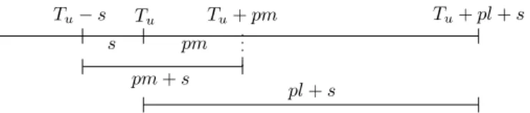
Proof Figure2shows all the relevant time instants for the proof. As in Lemma 4, consider any batchσuof sizel= |σu|of the GREEDYsolution, with starting timeTu,
and letσbe the first batch of the optimal solution OPTthat contains some jobs in
σu. Further, letm= |σu∩σ|. Below, we compare the total accumulated flow time
before and after timeTufor the jobs inσu, for both GREEDYand OPT.
Lemma4implies that no job inσucan complete beforeTuin OPT. Thus, until time Tu, the jobs inσuhave accumulated a total flow time ofF≤Tu(σu):=
Fig. 2 Important time instants in GREEDY’s competitiveness proof
in both GREEDY and OPT. Let FG≥REEDYTu (σu) denote the total flow time for the
jobs in σu after time Tu in the GREEDY solution, and FO≥PTTu(σu) the same quan-tity for the OPT solution. Further, we let FOPT(σu)=F≥
Tu
OPT(σu)+F≤
Tu(σu)and
FGREEDY(σu)=FG≥REEDYTu (σu)+F≤
Tu(σ
u)be the total flow time for the jobs in σu
in OPTand GREEDY, respectively. As σ finishes at least pm time units after Tu
(Lemma4), and all jobs inσumust have been released byTu, the total flow time of
OPTfor the jobs inσuafter timeTuis
F≥Tu OPT(σu)≥ Lemma4 m(pm)+ wait forσ (l−m)(pm)+ Observation5 1 2p(l−m) 2+(l−m)s =1 2(pl 2+pm2)+s(l−m). (2)
After timeTu, the GREEDYsolution further accumulates a total flow timeFG≥REEDYTu (σu)
=Pu=l(lp+s)for thel≥mjobs inσu. Now, ifσstarts atTu−sor earlier, then all jobs inσmust have been released atTu−sor earlier. Therefore, up until timeTu, themjobs inσu∩σalready yield an accumulated total flow timeF≤Tu(σu)≥sm
in this case. Thus we have
FGREEDY(σu) FOPT(σu) ≤ pl2+sl+F≤Tu(σu) 1 2(pl2+pm2)+s(l−m)+F≤Tu(σu) =1+ 1 2p ≥0 (l2−m2)+sm 1 2p(l2+m2)+s (l −m) ≥0 +F≤Tu(σ u) ≥sm ≤1+ 1 2p(l 2−m2)+sm 1 2p(l2+m2)+sl in this case.
Next, we consider the case in whichσ starts after Tu−s, say at starting time
Tu−s+τ, forτ >0. We still haveFG≥REEDYTu (σu)=l(lp+s) for GREEDY. In this
the bound (2) forF≥Tu
OPT(σu). Hence in this case,
FGREEDY(σu) FOPT(σu) ≤ 1 pl2+sl+F≤Tu(σu) 2(pl2+pm2)+s(l−m)+τ l+F≤Tu(σu) =1+ 1 2p(l 2−m2)+sm−τ l 1 2p(l2+m2)+s(l−m)+τ l+F≤Tu(σu) ≤1+ 1 2p ≥0 (l2−m2)+sm 1 2p(l2+m2)+s (l −m) ≥0 +τ l +F ≤Tu(σu) ≥m(s−τ ) ≤1+ 1 2p(l 2−m2)+sm 1 2p(l2+m2)+sl+τ (l −m) ≥0 .
So in both cases, we have
FGREEDY(σu) FOPT(σu) ≤1+ 1 2p(l2−m2)+sm 1 2p(l2+m2)+sl =1+ 1 2(l 2−m2)+ s pm 1 2(l2+m2)+ s pl .
Clearly,FGREEDY(σu)
FOPT(σu) ≤2 becausem≤l. Furthermore, note that sincelcan be as large
asn, this ratio comes arbitrarily close to 2 asnincreases, irrespective of the values of
sandp. Since FGREEDY(σu)
FOPT(σu) ≤2 holds for any batchσu of the GREEDYsolution, the
theorem follows.
2.2 A tight example for GREEDYfor largen
Consider the following instance: The first job arrives at time 0, then immediately afterwards (ε >0 later) a second job arrives. All otherk:=n−2 jobs arrive at time
s+2p+ε. Greedy will process the first two jobs in two separate batches, and then all other jobs in one batch. Thus, the flow time of the GREEDYsolution (omittingε) is
FGREEDY=(s+p)+2(s+p)+k(s+s+kp)=k2p+2ks+3s+3p.
We compare this solution with the following: The first two jobs are processed together in one batch starting atε. The other k=n−2 batches are split into √k
batches of size√keach (for simplicity, we assume thatk=n−2 is a square number). The total flow time of this solution (again omittingε) is
2(s+2p)+ √ k i=1 i√k(s+√kp)=2(s+2p)+1 2k 2p+1 2ks+ 1 2pk 3/2+1 2sk 3/2.
Hence we have FGREEDY FOPT ≥ 2k2p+4ks+6(s+p) k2p+ks+pk3/2+sk3/2+4(s+2p) = 2p+4s/ k+6(s+p)/ k2 p+s/ k+p/ k1/2+s/ k1/2+4(s+2p/ k2),
and this ratio approaches 2 asn increases (recallk=n−2). Thus, for arbitrary positive values ofsandp, and for sufficiently large values ofn, our analysis of the competitive ratio of GREEDYis tight.
2.3 Lower bounds for identical processing times
To complement the upper bound on the competitive ratio of our GREEDYalgorithm, we derive two lower bounds on the competitive ratio of any algorithm for the online BATCHFLOW problem, again with identical processing times. These bounds show that no online algorithm can be much better than GREEDYfor this setting.
For the following bounds, when we write that the adversary lets a job to be released
immediately aftert, we mean that the job’s release time ist+εfor an arbitrarily small
ε >0. For simplicity, we do not includeεin the calculations, but all proofs could be easily adapted by includingεand making it sufficiently small.
Theorem 7 No online algorithm for the online BATCHFLOWproblem with identical processing times can have a competitive ratio lower than
1+ 1 1+maxmin(p,s)(p,s) ≤
3 2.
Proof LetAbe any online algorithm with finite delay timeΔA for P= {1}. The adversary chooses release timesr1=0,r2immediately afterΔA, andrjimmediately
afterΔA+p(j−1)+s(j−2)forj∈ {3, . . . , n}, as depicted in Fig.3. Observe that an offline solution can avoid any waiting time forn−2 jobs: If job 1 and job 2 are processed together, the first batch has finished just when job 3 is released, so if job 3 is processed immediately, it will be finished just when job 4 is released, and so on until jobn. Thus,
FOPT≤
job 1 waits
ΔA +2(2p+s)+(n−2)·(p+s)=n(p+s)+ΔA+2p.
For bounding the flow time ofA’s solution, we examine for each jobj the earliest possible completion time thatAcan achieve.
By construction of the example,Acannot batch job 2 together with job 1, and starts processing job 1 at timeΔA, which completes atC1=ΔA+p+s. Hence, job 2 cannot start processing beforeC1, and thusC2≥ΔA+2p+2s. By induction, we show that for eachj∈ {3, . . . , n}, it holdsCj≥ΔA+pj+s(j−1)+min(p, s).
j=3:As batching job 3 together with later jobs will only increase job 3’s completion time, the earliest possible completion timeC3 is either achieved by batching job 3 with job 2, or by processing job 3 separately. The two possibilities yield completion times C3=ΔA+2p+s+ process jobs 2,3 2p+s =ΔA+4p+2s and C3=ΔA+2p+2s+p+s=ΔA+3p+3s,
respectively. We haveC3≥ΔA+3p+2s+min(p, s).
j−1→j:Note that batching more than two jobs would result in an idle time of more thanp+s, which is certainly not fastest possible. So, the fastest possible way to process jobj is to either batch it with jobj−1 or to process it separately. If jobj
is batched with jobj−1, then
Cj≥rj+2p+s=ΔA+p(j+1)+s(j−1).
If jobj is processed separately,
Cj ≥Cj−1+p+s≥ΔA+p(j−1)+s(j−2)+min(p, s)+p+s =ΔA+pj+s(j−1)+min(p, s).
Again, we see thatCj≥ΔA+pj+s(j−1)+min(p, s). Addingnj=1Fj= n j=1(Cj−rj), we get FA≥ job 1 ΔA+p+s+ job 2 2p+2s+ n j=3 (p+s+min(p, s)) =ΔA+np+p+ns+s+(n−2)min(p, s).
The competitive ratio can now be bounded as
FA FOPT ≥ ΔA+np+p+ns+s+(n−2)min(p, s) n(p+s)+ΔA+2p → p+s+min(p, s) p+s =1+ 1
1+maxmin(p,s)(p,s) forn→ ∞. Using a similar construction, we get the following lower bound.
Fig. 4 ForcingAto process all jobs separately. Waiting time is shown as dashed lines, batch processing time as solid lines
Theorem 8 No online algorithm for the online BATCHFLOWproblem with identical processing times can have a competitive ratio lower than
1+ 1 1+2ps ≤2.
Proof The following adversary can force every online algorithmAto process all jobs separately: Release job 1 and wait forΔA until A processes it, then immediately release job 2, wait forΔAuntilAprocesses it, and so on. Note that this causes every job except the first one to wait at leastp+s(see Fig.4). Furthermore, the intervals between the job release times are all at leastp+s(and exactlyp+sifAprocesses each job as soon as the previous batch finishes, i.e. allΔA=ΔA=. . .=0), except for the first intervalΔA, which can be smaller. The flow time ofA’s solution thus equals the batch processing time plus at leastp+swaiting time forn−1 jobs, giving
FA≥ processing n(p+s)+ waiting ΔA+(n−1)(p+s)=(2n−1)(p+s)+ΔA.
For bounding the optimal offline flow time, we consider the solution of batching job 1 and job 2 together, and processing all other jobs separately. Since each interval after job 2 is at leastp+s, and processing job 1 and job 2 together takes 2p+stime, job 3 needs to wait at mostp. Processing job 3 will hence complete no later thanr4+p, so job 4 has to wait at mostp, and so on. So, we can bound the optimal offline flow time as FOPT≤ΔA+ process jobs 1,2 2(2p+s) + waiting of jobs 3, . . . , n (n−2)p + process jobs 3, . . . , n (n−2)(p+s) =ΔA+2np+ns.
Thus, the competitive ratio is bounded by
FA FOPT ≥2p+2s− p+s−ΔA n 2p+s+ΔnA →1+ 1 1+2sp forn→ ∞.
2.4 Bounds on the competitive ratio with job reordering
The following theorem shows that no online algorithm can have a good worst case performance for the online BATCHFLOWproblem with general processing times, if the jobs do not need to be scheduled in the order they are given.
Theorem 9 For the online BATCHFLOW problem, no online algorithm can have competitive ratio better thann2.
Proof LetAbe any online algorithm. Consider an instance ofnjobs, where job 1 has processing timep, and jobs 2, . . . , nhave processing time 1 each, and are released immediately afterAstarts processing job 1 (after having delayed forΔAtime units). Note that any competitive algorithm must start processing job 1 after some finite time (otherwise, its competitive ratio is unbounded if no further job arrives after job 1). As each of the jobs 2, . . . , nhas to wait for job 1 to finish, the total flow time forAis
FA≥ΔA+n(p+s)+1
2(n−1)
2+(n−1)s,
where we used the lower bound from Observation5for optimally processing(n−1)
jobs of equal processing time arriving at the same time.
For OPT, consider the solution that first processes jobs 2, . . . , nin one batch, and after that processes job 1:
FOPT≤ΔA+n((n−1)+s)+p+s.
We assume in the following thatΔA≤p+s; ifΔA> p+s, then our bound for
FA increases, but we can decrease the bound forFOPT because OPTcan complete
job 1 even before the other jobs are released, and then process all other jobs in one batch. We thus have
FA≥np+1 2n 2+ 2ns−n−s+1 2 and FOPT≤2p+2s+n 2−n+ns. It is easily verified that
n 2−ε ·FOPT≤FA if we choosep≥ 1 4ε(n 3+n2s+2n+2s+2εn).
Theorem9shows that for the general setting, there is no online algorithm with a sub-linear competitive ratio. However, we will see in the following that all so-called non-waiting algorithms, a class to which the GREEDYalgorithm belongs, are strictlyn-competitive, i.e., are at most a factor 2 away from the lower bound. We call an online algorithm non-waiting if it never produces a solution in which there is idle time while some jobs are pending.
Theorem 10 Any non-waiting online algorithm for the online BATCHFLOWproblem is strictlyn-competitive.
Proof LetAbe any non-waiting online algorithm. Consider any jobi, and letσube
the batch which contains jobi. Furthermore, letJbe the set of all jobs not contained inσu. The flow time of jobiisFi =Ci −ri =Tu+Pu−ri. The longest possible
interval during whichσu needs to wait (i.e. the machine is busy) in a non-waiting
algorithm’s solution iss|J| +j∈Jpj. So, for a non-waiting algorithm,Tu−ri ≤ s(n−1)+ j∈J pj. Hence, Fi≤Pu+s(n−1)+ j∈J pj≤sn+ n j=1 pj.
Thus, the total flow time forA’s solution is
FA= n i=1 Fi≤n2s+n· n j=1 pj.
We now turn to the optimal solution OPT. Clearly, each jobj has flow timeFj ≥ pj+s, as the batch processing time is inevitable. Thus, the flow time of OPTis at
least FOPT= n j=1 Fj≥ns+ n j=1 pj.
Comparing the total flow timesFAandFOPTcompletes the proof.
Observe that this upper bound proof does not make use of the fact that the reorder-ing of jobs is allowed. Thus, addreorder-ing a fixed job sequence constraint does not affect the validity of Theorem10. Note that this is not true for Theorem9.
We remark that the online non-preemptive scheduling problem with release times known from the literature (see e.g. Epstein and van Stee2003) is a special case of the online BATCHFLOWproblem. Thus, theΘ(n)upper bound for the former problem is implied by our Theorem10.
3 Discussion
We studied the online BATCHFLOWproblem 1|rj, sf =s, F=1|
Fj, and
investi-gated this problem for the case of identical processing times and for general process-ing times.
We shortly mention here further results we can prove (see Gfeller et al.2006), whose detailed explanations and proofs are omitted in this paper. With a fixed job sequence (but arbitrary processing times), no online algorithm for the online BATCH -FLOW problem can have a constant competitive ratio. The general offline BATCH -FLOWproblem is NP-complete, even with machine setup times=0. When the job sequence is fixed, there exists a dynamic programming-like algorithm with polyno-mial running time.
References
Albers S, Brucker P (1993) The complexity of one-machine batching problems. Discrete Appl Math 47:87– 107
Bein W, Epstein L, Larmore L, Noga J (2004) Optimally competitive list batching. In: 9th Scandinavian workshop on algorithms theory (SWAT). Lecture notes in computer science, vol 3111. Springer, Berlin, pp 77–89
Chen B, Deng X, Zang W (2004) On-line scheduling a batch processing system to minimize total weighted job completion time. J Comb Optim 8:85–95
Cheng T, Kovalyov M (2001) Single machine batch scheduling with sequential job processing. IIE Trans Sched Logist 33:413–420
Coffman E, Yannakakis M, Magazine M, Santos C (1990) Batch sizing and job sequencing on a single machine. Ann Oper Res 26:135–147
Deng X, Poon C, Zhang Y (2003) Approximation algorithms in batch processing. J Comb Optim 7:247– 257
Deng X, Feng H, Zhang P, Zhang Y, Zhu H (2004) Minimizing mean completion time in a batch processing system. Algorithmica 38(4):513–528
Divakaran S, Saks M (2001) Online scheduling with release times and set-ups. Technical Report 2001-50, DIMACS
Epstein L, van Stee R (2003) Lower bounds for on-line single-machine scheduling. Theor Comput Sci 299(1–3):439–450
Gfeller B, Peeters L, Weber B, Widmayer P (2006) Single machine batch scheduling with release times. Technical Report 514, ETH Zurich, April 2006
Lee C, Uzsoy R, Martin-Vega L (1992) Efficient algorithms for scheduling semiconductor burn-in opera-tions. Oper Res 40(4):764–775
Poon C, Yu W (2004) On minimizing total completion time in batch machine scheduling. Int J Found Comput Sci 15(4):593–607
Poon C, Yu W (2005a) A flexible on-line scheduling algorithm for batch machine with infinite capacity. Ann Oper Res 133:175–181
Poon C, Yu W (2005b) On-line scheduling algorithms for a batch machine with finite capacity. J Comb Optim 9:167–186
Potts C, Kovalyov M (2000) Scheduling with batching: a review. Eur J Oper Res 120:228–249 Webster S, Baker K (1995) Scheduling groups of jobs on a single machine. Oper Res 43(4):692–703 Zhang G, Cai X, Wong C (2001) On-line algorithms for minimizing makespan on batch processing