Real option models for simulating digester system adoption on livestock farms in Emilia-Romagna

1

R

EAL

O

PTION MODELS FOR SIMULATING DIGESTER SYSTEM ADOPTION ON LIVESTOCK FARMS IN

E

MILIA

-R

OMAGNA

FABIO BARTOLINI, VITTORIO GALLERANI ANDDAVIDE VIAGGI

Department of Agricultural Economics and Engineering Alma mater studiorum - University of Bologna Corresponding author [email protected]

Paper prepared for presentation at the 114th EAAE Seminar

‘Structural Change in Agriculture’, Berlin, Germany, April 15 - 16, 2010

Copyright 2010 by author(s). All rights reserved. Readers may make verbatim copies of this document for non-commercial purposes by any means, provided that this copyright notice appears on all such copies. The research reported in this paper was funded by the European Commission within the project “Assessing the multiple Impacts of the Common Agricultural Policies (CAP) on Rural Economies” (CAP-IRE), 7th Framework Programme, contract n. 216672 (www.cap-ire.eu). However the paper does not necessarily reflect the views of the EU and in no way anticipates the Commission’s future policy in this area.

2

A

BSTRACT

Innovation and new technology adoption represent two central elements for the enterprise and industry development process in agriculture. The objective of this paper is to develop a farm-household model able to simulate the impacts of uncertainty in SFP, the selling price of energy and agricultural product prices parameters on the adoption of methane digester for biogas production. The model implemented is based on a real option approach that includes investment irreversibility and stochasticity in relevant parameters. The results show the relevance of uncertainty in determining the timing of adoption and emphasise the importance of predictability as a major component of policy design.

Keywords: real options; methane digester; biogas; investment; uncertainty

1.

I

NTRODUCTION AND OBJECTIVES

New technology adoption and innovation diffusion represent two central elements for the enterprise and industry development process in all sectors of the economy. Innovation is one of the main drivers of economic growth and an important instrument for achieving sustainability and cohesion (Ghazalian and Furtan, 2007). Innovation adoption and the re-organization of agri-food chains are two of the Health Check priorities. In addition, with the Health Check, the issues of climate change and the production of bio-energy have been included in the second pillar priorities, as well as other environmental priorities (water management and biodiversity preservation). In order to match these new priorities, the EU has stimulated Member States to implement measures with the objective to promote the biogas or bio energy productions, adopting incentive mechanisms aimed to co-fund the investment costs (Swinbank, 2009). Among farm innovation options, the adoption of technologies for the production of energy from renewable sources is hence a relevant topic in the European Policy Agenda and represents an important opportunity for farmers with regard to income differentiation and stabilization. On-farm energy production is generally realized in several ways, however biogas production through methane digester systems have a higher potential compared to the other sources of bio-energy (Piccinini et al., 2008). The production of biogas is generally obtained by using by-products derived from animals (e.g. slurry or manure) or plants (e.g. pectin, molasses) or from specific crops (e.g. maize or sorghum). With the implementation of energy

3 production systems, farm and household energy needs can be provided by on-farm activities and, in addition, energy surpluses can be sold.

Biogas production using slurry and manure anaerobic digestion is the main source of energy production by the farm, contributing to the abatement of CO2 emissions (Clemens et al., 2006). In the last years the number of biogas product implantations is increasing over time, also as a consequence of the improvement in the yield of methane and with the introduction of the combined substrate, using by-products or specific crops (Clemens et al., 2006).

The objective of this paper is to develop a dynamic farm-household model able to simulate the impacts of uncertainty on digester system adoption. The main causes of uncertainty addressed are SFP developments after 2013, the selling price of energy and volatility of agricultural product prices. The model implemented is based on a real option approach that includes investment irreversibility and stochasticity of decision variables, allowing for an improved analysis of the profitability of investments in bio-gas production, and the timing of decisions regarding investment. The paper is structured as follows. In the next section we describe the theoretical model; in the following we describe the methodology used and then the case study to which the empirical methodology is applied. This is followed by a result section and a discussion.

2.

T

HEORETICAL MODEL

Real options models are an emerging subject in the economic literature concerning investment behaviour. The model features allow describing in a better way than capital budgeting tools an investment choice carried out under conditions of irreversibility ad uncertainty (Dixit e Pindyck, 1994; Schwartz and Trigeorgis, 2004). Such approach allows for the improvement of the investment evaluation, taking into account the optimal timing on which the investments is undertaken, in addition to the classical elements of investment profitability (Blyth et al., 2007). The opportunity to postpone the investment until circumstance turn favourable can determine an increment of investment value. In fact, the opportunity to delay an investment can be treated as a financial call option (Trigeorgis, 1988).

Uncertainties in methane digester investment evaluation are due mainly to the following sources: a) prices energy fluctuation for consumption; b) availability and cost of agri-food by-products or other substrate used in the digestion process; c) limitation and costs of the disposal of digested waste products; d) prices of energy sold by the farm (Blyth et al., 2007; Stokes et al., 2008).

4 Under condition of uncertainty and investment irreversibility the real-options approach enables to quantify the Net Present Value (NPV) increment due to the option to delay the methane investment in a following period, when the farmer have access to more information on the exogenous uncertain variables determining investment profitability (Stokes et al., 2008).

Such approach is presented in figure 1, with an example in which the choice to invest can be undertaken during two distinct periods.

FIGURE 1

Under such assumption, the adoption of the new technology can be interpreted as a discrete choice, which the farmer can take in either the first or the second period. Investment in new technology can be realised during the first period t1 or during the second period t2. The choices to invest during the first period lock-in the farm in the production of energy also during the second period (situation 1). Lock-in is determined by high investment and sunk costs and by the irreversibility of the investment (Carruth et al., 2000). However, the farmer can also delay the investment until he gets more information about the hypothesised uncertain variables and then will realise the choice during the second period. The delay allows the farmer to observe the value of such variables that was not known in the previous period and, if such variables will be favourable to the methane digester in terms of profitability, then the farmer will carry out the investment in period t2 (situation 2). Otherwise, if the value of the uncertain variables will be not favourable to the profitability of the investment in the methane digester, then the farmer will choose not to invest (situation 3).

As previously explained, investment in the methane digester system is based on a discrete choice among three different strategies. The optimal strategy will be the one with a higher NPV of the cash flow over both periods.

Formally, this can be summarised as: NPV=max

(

NPV₁,NPV₂,NPV₃

)

, where NPV₁, referring to figure1 is the net present value of the cash flow in situation 1; NPV₂ is the net present value of the cash flow in situation 2 and finally NPV₃ is the net present value of the cash flow in situation 3. (Equation 1, 2, 3).

(

)

∑

∑

+ + + − + + + + − = 1 0 2 1 1 1 2 2 1 1 ) 1 ( 1 ) 1 ( t t t t t t inn t inn t t inn i cf cf i cf k NPV

γ

γ

(1)

5

(

)

_       + − +         + + + − + + =

∑

∑

∑

+ + + + + 2 1 1 1 2 2 1 1 1 2 1 1 0 1 2 ) 1 ( 1 ) 1 ( ) 1 ( ) 1 ( t t t t t t t t t t inn t t t t t i cf i cf i k i cf NPV

γ

γ

(2)

(

)

∑

∑

+ + + − + + + = 1 0 2 1 1 1 2 2 1 3 ) 1 ( 1 ) 1 ( t t t t t t t t t i cf cf i cf NPV

γ

γ

(3) Where: t

cf = cash flows of a generic year t, with t=t1 if years are belonging to the first period and t =t2 if year are belonging to the second period;

k = cost of investments; i = discount rate;

γ = probability to have a methane digester favourable state of nature; 2

2 , t t inn cf

cf = cash flow of a generic year t when t=t2 and stochastic variable values are favourable to methane digester adoption;

2 2

, t t inn cf

cf = cash flow of a generic year t when t=t2 and stochastic variable values are unfavourable to methane digester adoption.

inn = subscript that means the adoption of the methane digester.

In each period the investment would be carried out at the beginning of the period, i.e. t=0or t=t1. The methane digester adoption is subject to uncertainty in the second period. This assumption implies stochastic cash flows value during the second period. Following Dixit and Pyndick (1994) we assumed that the annual cash flows can follow a Brownian Motion with drift, so that

dz dt cf

dcft =µ t ±σ , where dcft is the instantaneous value of the cash flow; µtcft dt is the expected cash flow value; µ is drift,

σ

is the volatility, and dz is a Wiener process with mean zero and independent increments.

Under such approach, it is possible to differentiate two values of cash flows, one favourable to the methane digester investment (cft ) and the other unfavourable (cft ). Such two values are generated assuming that the random variable generated from the Wiener process can have positive or negative value in order to allow adding or removing in each moment t2 the same amount from the expected value: formally cft =

µ

cf t dt+

σ

dz and cft =

µ

cft dt−

σ

dz.

6

3.

E

MPIRICAL ANALYSIS

The empirical analysis has followed three steps: 1) Identification of the representative farm; 2) Building of the household model;

3) Modelling uncertainty in exogenous variables.

3.1IDENTIFICATION OF THE REPRESENTATIVE FARM

The model has been tested to three representative farm households, specialised in livestock production, in the Province of Bologna (Emilia Romagna, Northern Italy). The three representative farms have been obtained using cluster analysis starting from the CAP-IRE1 database with 300 farm household interviews realised in the Province. A subsample of 31 farm households which self identified livestock as their main farming specialisation was selected for the clustering analysis. Applying Cluster Analysis2 to the 31 farms, three groups of livestock farms were identified. The main characteristics of the groups resulting from cluster analysis and the frequencies in the database are presented in Table 1.

TABLE 1

The three clusters generated represent three different livestock systems. Cluster 1 represent a small farm, characterised by a low number of animal reared, having, in addition, an equal weight of beef and dairy cows rearing. Household members involved in farming activity are less than two and less than one part-time employee is involved as non-household farm worker. Land cultivated is small compared to the other two clusters with a surface of 22.59 Hectares.

1

CAP-IRE is the acronym of a 7th Framework Program Project titled Assessing the multiple Impacts of the Common Agricultural Policies on Rural Economies. Furtherinformation is available on the following web-site: http://www.cap-ire.eu/default.aspx.

2

A non-hierarchical cluster analysis k-means was applied. The variables used for cluster analysis are the heard number for both dairy and beef livestock and the Usable agricultural Area. The best clustering was obtained by that one with higher Calinski/Harabasz pseudo-F value.

7 Cluster 2 and Cluster 3 are intensive livestock farms, with a similar number of cows reared but strongly specialised in beef and in dairy production respectively. Total labour used on-farm is quite similar among the two clusters, but the distribution between household and external labour is rather different. In fact, cluster 2 has a strong use of household labour (3.5 full time equivalents) and cluster 3 has less use of household labour but higher value of external labour (1.50 full time equivalents). Finally, the amount of land possessed is strongly diversified among the cluster2 and 3, with a higher amount of land owned for the second cluster and homogenous division between land owned and land rented–in for the third cluster.

The technical and economic coefficients for the methane digester have been collected through expert interviews. Five alternative methane digester systems have been considered, differentiated on the basis of maximum energy production (from 108 to 972 kW/h). Such systems have implantation costs, annual fixed costs and labour needed different among each other and increasing with the size of the plant.

3.2BUILDING OF THE HOUSEHOLD MODEL

The empirical analysis was conducted using a Dynamic Farm Household Model with the objective to maximise the Net Present Value of the cash flow over the next 20 years. Model has been hypothesised be structure in two time periods the first period ( 1t ) include the years between 2010-2013 and the second period ( 2t ) included years 2014-2030. Farm household models can enable to maximise the utility function generated by the household income, the household leisure time and the household consumptions (Taylor and Adelman, 2003). The simulation of a farm household behaviour rather than using a capital budgeting approach, enabled to take into account whole farm adaptations in the decision to adopt an energy production technology. In fact, the investment in a methane digester system has been simulated considering the connections between livestock activity, crop cultivation and labour allocations among such activities. Household has been supposed to maximising the whole household NPV, subject to consumption and leisure constrains. In fact, with reference to equation 1, 2 and 3 the cash flow in a generic year t (cf_t) is equal to the algebraic sum

of on-farm income (Πt_onfarm), off-farm income (Πt_offfarm) and the eventual loan repayment ( t r C ). Formally: rt t farm ff o t onfarm t C cf =Π +Π −

On-farm income is obtained by summing the crop production incomes (π_ct), the milk production

income(πmt ), the energy surplus ( t e

8 investment in the methane digester ( t

RDP ); and the single farm payments received (SFPt), minus the cost of external labor purchased (Clt) and the cost of energy used by the farm-household (

t eb C ).

Formally the on-farm profit is ebt

t l t t t e t m t c t onfarm = + + +RDP + SFP −C −C Π

θ

π

π

θ

π

θ

.

Off-farm income is obtained by summing the financial income (Fint), pensions received by household members (Penst) and the income obtained by allocating household labor to off-farm activity (Oint). Formally the off-farm income is Πt_offarm =Fint +Penst +Oint.

With reference to equation 1, the cash flow of a generic year in the first period (t1) and in the second period (t2) are: cf_innt1 =Πt_onfarm1_i +Πt_o1_fffarm−C_rt1 and cf_innt2 =Πt_onfarm2_i +Π_ot2_fffarm −C_rt2.

Where:

(

1 1

) (

1 1

)

1 1 1 1 1 1 _ 1 ) 1 ( t t sb e t t e t q m m t m c t l c t c t c c t c i t onfarm x i r cp C C + i p −C −C + i ep −C −C +RDP +SFP      − − − = Π

∑

(4)

(

)

(

)

(

)

(

)

(

)

(

)

(

)

(

1

)

(

(

(

1

)

)

)

1 ) 1 ( 2 2 2 2 2 2 2 2 2 2 2 2 _ 2 t t sb e t e t e t e t q m m t m i t l c t c t c t c c t c i t onfarm SFP SFP C C ep ep i C C p i C C cp cp r i x γ γ γ γ γ γ − + + − − − + + + − − +       − − − + − = Π

∑

(5)

With reference to equation 2, the cash flow of a generic year in the first period (t1) and in the second period (t2) are cft1 =Πt_onfarm1 +Πt_o1_fffarm−C_rt1 and

(

)

(

)

(

2_ 2

)

2 2 2 1 rt t farm ff o t onfarm i t onfarm t inn C cf =

γ

Π + −

γ

Π +Π − . Where:

(

1 1

)

1 1 1 1 1 1 ) 1 ( _mt _{m m q}n t _ebt c n l c c t c c t c t onfarm x i r p C C + i p −C −C +SFP −C      − − − = Π

∑

(6)

(

)

(

₂ 2

)

₂

(

2

)

2 2 2 2 2 2 _ 2 ) 1 ( t t sb e t t e t q m m t m c t l c t c t c c t c i t onfarm SFP RDP C C ep i C C p i C C cp r i x + + − − + + − − +       − − − = Π

∑

(7)

(

2 2

)

(

2

)

2 2 2 2 2 2 ) 1 ( ebt t t q m m t m c t l c t c t c c t c t onfarm x i r cp C C + i p −C −C + SFP −C      − − − = Π

∑

(8)

With reference to equation 3 the cash flow of a generic year in the first period (t1) and in the second period (t2) are: cft1 =Πt_onfarm1 +Πt_o1_fffarm−C_rt1; cft2 =Πt_onfarm2 +Πt_o2_fffarm−C_rt2

9

(

1 1

)

1 1 1 1 1 1 ) 1 ( _mt _{m m q}t t _ebt c t c c c t c c t c t onfarm x i r p C C + i p −C −C +SFP −C      − − − = Π

∑

(9)

(

)

(

)

(

)

(

)

(

)

(

)

(

2 2

)

2 2 2 2 2 2 2 2 2 1 1 ) 1 ( t eb t t t q m m t m c t l c t i t c t c c t c t onfarm C SFP SFP C C p i C C p c cp r i x − − + + + − − +       − − − + − = Π

∑

γ γ γ γ (10) With : t c

x = surface of crop c on the year t; c

i = yield of the crop c; t

c

r = crop yield reused as substrate for energy production; t

m

i = amount of milk sales on the year t; t

e

i = amount of energy sales by the year t; c

C = production cost of crop c, m

C = milk production cost; e

C = energy production cost; sb

C

= cost of purchase of by-products for energy production; t l C = rent cost; t q C

= milk quota rent cost; t

eb C

= energy purchasing cost; t

c

cp = crop prices for the year t; m

p = milk price; t

e

ep = energy surplus price for the year t;

γ = probability to have favourable context conditions for methane digester; 2

t c cp ; t2

c

cp = crop prices favorable and not favorable for the year t during the second period; 2

t c ep ; t2

c

ep = = energy prices favorable and not favorable for the year t during the second period; 2

t

SFP ;SFPt2= Single Farm Payment favorable and not favorable for the year t during the second period.

Constraints applied to the model are: rotation constraints, cow-house dimension; manure and slurry spreading constraints. A dimensional constraint was applied to the biogas digester system, in order to satisfy the substrate quantity needed by the digested choice among the five different typologies.

10 Such constraint, binds the farmer to buy on the market the by-products needed to compensate the lack of substrate needed by the digester. Finally a liquidity constraint has been applied in order to force the farm to obtain a loan and to pay an interest on the loan, when cash is insufficient to buy the methane digester systems.

3.3MODELLING UNCERTAINTY

The model has three stochastic parameters: the amount of SFP received by the farm; the level of agricultural prices and the energy sale prices. This implies that the farmer at time t1 (first period) knows the average of amount of SFP received by the farm; level of agricultural prices and energy prices and the oscillation for each of the stochastic parameters. Formally uncertainty can be expressed by: St2 =Sedt±σdz. Where St2 is the expected value for a generic year belonging to the second period ( 2t ) of each stochastic parameters; Se is the average or known value during the first period;

σ

is the oscillation (known during the first period) and dz is a random variable uniformly distributed with minimum value 0 and maximum value 1. Through a Monte Carlo Approach, dz has been simulated as an N x M matrix of random values, where M represents the times on which each stochastic parameters changes over time and N represents the number of interactions generated by the Monte Carlo simulation3.

The general approach has further specifications depending by the stochastic parameter considered. For the SFP variablesSe is the expected value of the single farm payments after 2014, that is equal at half of the current single farm payment4;

σ

is the oscillation with value equal to S. Such specification allows to determine a random value of single farm payment (SFPt2) that is uniform distributed with the maximum and minimum value being respectively the current SFPpayments and 0. The amount of SFP change during the second period twice coherently with the expected European Union CAP program (M_iSFP₁ ;M_iSFP₂ ), where M_iSFP₁ is the sub-set that includes the years

2014-2019 and MiSFP2 is the sub-set that includes years 2020-2030. Note that under such formulation

at time t2 the variable SFPt2can have two values for each sub-set MiSFP: the high value

(SFPt2 =Sedt+σdz) and the low value SFPt2 =Sedt−σdz.

For the energy price variable we have the following specification: Se is the current price of energy;

σ

is the standard deviation obtained by placing as the maximum value the current energy price and

3

Monte Carlo Model Simulation has been carried out using MATLAB software

4

11 as the minimum value the minimum guaranteed prices by Italian Legislation. Such specification allows to determine a random energy price variable ( t2

ep ) with a uniform distribution with the maximum and minimum values equal respectively to the current energy prices (0.28 per kW) and 0.22 (€ per kW) that correspond to the minimum guaranteed prices. Energy prices have been assumed to change during the second period six times, coherently with schemes of guaranteed prices, that are redefined each three years by the public administration (Mep_j1,...,Mep_j6): Mep_j1 is the

sub-set that includes the years 2014 -2016 by steps of three years; the last sub-set is ep j

M ₆, that

includes years 2029-2030. Note that under such formulation at time t2 the variable ept2can have

two values for each sub-set Mepj : the high value (ep S dt dz e t σ + = 2

) and the low value dz

dt S

ept2 = e −σ .

For the crop prices variable we have the following specification: c c e

c S S 2009µ

= , where Sc2009is a vector of dimension c x 1 with the price level placed at year 2009 and c is the set of crops considered in the simulation; µcis the annual drift

5

; σc is a vector of dimension c x 1 of the

standard deviations6. Such specification allows to determine a random crop prices variable (cpct2) with a uniform distribution with a maximum value cp_ct2 =S_c2009µ_c +σ_c and a minimum

valuecp_ct2 =S_c2009µ_c−σ_c. Crop prices have been assumed changing during the second period each

year until 2030, so we will have thirty sub-set s(Mcp_j1,...,Mcp_j30). Note that under such formulation at

both time t1 and t2 the variable ec_ctcan have two value for each sub-set (that only in this case is equal to the years): the low value that is favorable to methane digester adoption, (cpt_c=S_c2009µ_c+σ_c) and the high value that is unfavorable to the methane digester adoption

(cpt_c=S_c2009µ_c+σ_c).

5

Drift has been calculated as percentage of annual change to obtain the foresee price levels that are presented in the OECD-FAO Agricultural Outlook 2009 report.

6

Standard deviation has been calculation using the foresee prices from year 2009-2018 present in the OECD-FAO Agricultural Outlook 2009 report.

12

4.

R

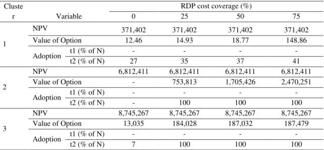
ESULTS

The results of the model are presented in Table 2, Table 3, Table 4 respectively for SFP, crop prices and energy prices, each results being parameterised on different contributions of RDP support (in percent on the value of the digester investment). A single model was run for each independent stochastic parameter; Table 2 presents the results with uncertainty in SFP.

TABLE 2

For each cluster, the average value of the Net Present Value and the average of the Value of Option due to the choice to delay the adoption in the second period are presented. The NPV is the net present value of the cash flows when the decision is made in time 1. Such a decision is concerned on both the adoption of technology during time 1 and the non-adoption in time 1 and time two. The value of options the increment of NPV obtained delaying the choice and adopting the innovation during the second period. Values of Option are presented in the tables as the average over all interactions (N). In addition, the percentages of adoption in each period over the total of number of interaction (N) for each cluster are presented.

Under uncertainty in the CAP, the NPV is rather homogeneous for the given percentage of cost coverage by RDP, but is strongly differentiated across cluster. Cluster 1 has a lower value in NPV compared to the other, and cluster 2 and cluster 3 have NPV 20 times and 30 times higher than the cluster 1. Such result is due to lower farm dimension and the less specialisation compared to the other two clusters.

The value of option for cluster 1 is positive for all RPD cost covered that implies profitability in the investment if realised during the second period and under favourable conditions. However, such value is quite low (maximum value of 148.86 €) that implies that in only few interaction has been adopted the methane digesters.

The value of option for cluster 2 have a positive value only for a value of RDP cost covered higher than 25%. This implies that without RDP in this cluster the methane digester system will be never adopted, even having more information about SFP. Increasing the RDP cost coverage the value of option increases strongly. In fact with the 75% of covering the cost the value of option for cluster 2 is equal to 2,470,251 €, that implies a very high profitability in the adoption of the methane digester

13 during the second period. In fact with percentage cost coverage higher than 25% in all interactions have been adopted the methane digester.

Finally the value of option for cluster 3 has a positive value for all percentages of cost coverage by RDP. Such value is quite constant across RDP investment cost covering, which implies a substantial indifference at the RDP cost covering by the cluster 3.

Uncertainty in SFP has a very strong negative effect on the adoption of new technology in the first period especially for cluster 2 and cluster 3. On these clusters the percentage of adoption is 100% that implies a decision to invest strongly dependent on the information available, concerning the amount of SFP.

Table 3 present the results with uncertainty in crop prices.

TABLE 3

The choice to adopt methane digester under uncertainty in crop prices follows the same tendencies of uncertainty in SFP. All clusters have a positive value of option that means profitability in delaying the adoption of methane digester when farm holds more information about the future prices. Cluster 2 and Cluster 3 without any RDP payments do not find profitability to invest in methane digester neither in the first or second period. The value of option for cluster 1 and cluster 2 is strongly different from the value of option under uncertainty in SFP. Cluster 1 has a little higher value of option as a consequence of higher profitability in adopting the methane digester system due to the high weight of the crop selling on the household income. Differently, cluster 2 value of option is very low to the value of option under uncertainty in SFP, as consequences of less weight of the crops prices on the on-farm income. This implies that uncertainty in crop prices have less negative effect of postponing investment in cluster 2 than uncertainty in SFP.

In table 4 the results with uncertainty in energy prices are presented.

TABLE 4

The choice to adopt methane digesters under uncertainty in energy prices has the same trends of the other stochastic parameters. Option value increasing strongly with higher value of RDP percentage of cost coverage. This implies that the uncertainties in energy prices are as well relevant to delay the

14 investment in the second period, but investment under favourable conditions is strongly profitable. Even with minimum guaranteed prices, and not market prices, the uncertainty in energy price determines a strong delay to methane digester adoption.

5.

D

ISCUSSION

The results show the relevance of uncertainty in determining the timing of adoption. In particular, the results highlight the relevance of crop prices, SFP and uncertainty with regard to the selling price of energy on the decision to adopt the new technology. Such uncertainty has the effect of postponing the investment until farmers have more information. Uncertainty with regard to policy scenarios after 2013 has a negative effect on the adoption of the new technology; in fact, for great part of models, the farmers postpone the decision to adopt methane digester until after 2013. The results emphasize that decisions to adopt the new technology, and the timing of such decisions, depend on the quality of the information available, as well as the length of the policy reform process. In particular, they highlight the importance of “predictability” as a major policy feature and component of policy design facing a strongly uncertain context.

The main policy implications derived from these results can be identified in four main areas. First, the need to reduce policy uncertainty and delay, particularly as local voluntary measures are concerned, with strongest emphasis on quantified policy objectives and smoothness of administrative procedures leading to investment implementation. Secondly, it would be advisable to reinforce (or build) links between investment support measures and uncertainty reducing measures (such as insurance), in order to prevent excessive exposition for farmers with the strongest intention to invest and encourage a more timely reaction by farmers facing funding opportunities. Thirdly, higher attention should be placed on the coordination between agriculture and energy policies, in order to minimise uncertainty and particularly to stabilise effects coming from joint negative conditions. Finally, RDP payments are very important instrument to incentive the innovation adoption and diffusion also under uncertainty in decision variables, in particular because such payments are cert although parameterised.

The main limitations of the model rests in its strong simplification compared with reality, at least as the timing of the processes is concerned and for the treatment of uncertainty.

This suggested a number of potential developments in the direction of improving both the timing on which decisions can be undertaken, including uncertainty in other decision variable (i.e, technology

15 improvement, different investment cost over time or prices, prescription or constraint) and to simulate uncertainty using different combination of uncertain parameters with an explicit correlation between each other.

R

EFERENCES

Blyth, W., Bradley, R., Bunn, D., Clarke, C., Wilson, T., and Yang, M. (2007). Investment risks under uncertainty climate change policy. Energy Policy 35: 5766-5773.

Carruth, A., Dickerson, A. and Henley, A. (2000). What do We Know About Investment Under Uncertainty? Journal of Economic Surveys 14: 119-154.

Clemens, J., Trimborn, M., Weiland, P., and Amon, B. (2006). Mitigation of greenhouse gas emissions by anaerobic digestion of cattle slurry. Agricultural, Ecosystems and Environment 112: 171-177.

Dixit, A., and Pindyck, R. (1994). Investment under Uncertainty Princeton. Princeton University Press.

Ghazalian, P.L., and Furtan, W.H. (2007). The Effect of Innovation on Agricultural and Agri-food Exports in OECD Countries. Journal of Agricultural and Resource Economics 32:448-461.

Mcdonald, R. and Siegel, D. (1986). The Value of Waiting to Invest. The Quarterly Journal of Economics, 101, 707-728.

Piccinini, S., Soldano, M., and C., Fabbri (2008). Le scelte politiche energetico-ambientale lanciano il biogas. L’informatore agrario 3: 28-32.

Schwartz E.S. and Trigeorgis L. (2004). Real Options and Investment under Uncertainty. In Schwartz E.S. and Trigeorgis L. (eds) Real Options and Investment under Uncertainty – Classical Readings and Recent Contribution. The MIT Press:1-16._

Stokes, J.R., Rajagopalan, R.M., and Stefanou, eS.E. (2008). Investment in a Methane Digester: An Application of Capital Budgeting and Real Options. Review of Agricultural Economics 30: 664-676.

Swinbank, A. (2009). EU Policies on Bioenergy and their Potential Clash with the WTO. Journal of Agricultural Economics, 60: 485-503.

16 Taylor, E. and Adelman, I. (2003). Agricultural Household Models: Genesis, Evolution and Extensions. Review of Economics of the Household 1: 33-58.

Trigeorgis L. (1988). A Conceptual Options Framework for Capital Budgeting. Advances in Future and Options Research 3: 145-167.

17

Figure 1 timing of the methane digester adoption

New technology adoption

Choice delayed

Lock-in

t1 t2

New technology adoption

1

2

3 Choice delayed

18

Table 1 – Group Characteristics and Frequencies

Group Code dairy cows (#) beef cows (#) hh labour ( # full time equivalent) no-hh labour (# full time equivalent) Land owned (ha) Land rented-in (ha) Frequency (%) c_1 6.67 4.96 1.96 0.25 12.46 10.13 77.42 c_2 - 130.00 3.50 1.00 192.50 10.00 6.45 c_3 126.00 2.00 2.30 1.50 45.20 36.00 16.13 All 49.96 37.29 2.18 1.05 48.00 21.81 100.00

Table 2 – Results with uncertainty in SFP, with number of interaction N=1000 (€ per farm)

Cluste r Variable RDP cost coverage (%) 0 25 50 75 1 NPV _{371,402 371,402 371,402 371,402} Value of Option 12.46 14.93 18.77 148.86 Adoption t1 (% of N) - - - - t2 (% of N) 27 35 37 41 2 NPV 6,812,411 6,812,411 6,812,411 6,812,411 Value of Option - 753,813 1,705,426 2,470,251 Adoption t1 (% of N) - - - - t2 (% of N) - 100 100 100 3 NPV 8,745,267 8,745,267 8,745,267 8,745,267 Value of Option 13,035 184,028 187,032 187,479 Adoption t1 (% of N) - - - - t2 (% of N) 7 100 100 100

Table 3 – Results with uncertainty in crop prices, with number of interaction N=1000 (€ per farm)

Cluster Variable RDP cost coverage (%) 0 25 50 75 1 NPV _{368,241 368,241 368,241 368,241} Value of Option 1,262 1,494 2,139 3,282 Adoption t1 (% of N) - - - - t2 (% of N) 15 25 37 42 2 NPV 6,822,501 6,822,501 6,822,501 6,822,501 Value of Option - 361,888 837,372 1,230,459 Adoption t1 (% of N) - - - - t2 (% of N) 100 100 100 3 NPV 8,743,765 8,743,765 8,743,765 8,743,765 Value of Option - 184,554 187,977 188,292 Adoption t1 (% of N) - - - - t2 (% of N) - 100 100 100

19

Table 4 – Results with uncertainty in energy prices, with number of interaction N=1000 (€ per farm)

Cluster Variable RDP cost coverage (%) 0 25 50 75 1 NPV 371,473 371,473 371,473 371,473 Value of Option 436 468 685 920 Adoptio n t1 (% of N) - - - - t2 (% of N) 28 30 40 43 2 NPV 6,812,411 6,812,411 6,812,411 6,812,411 Value of Option - 884,619 1,826,051 2,468,139 Adoptio n t1 (% of N) - - - - t2 (% of N) 100 100 100 3 NPV 8,745,432 8,745,432 8,745,432 8,745,432 Value of Option 1,862 29,941 165,215 186,924 Adoptio n t1 (% of N) - - - - t2 (% of N) 1 16 89 100