Computing Inferences for Large-Scale
Continuous-Time Markov Chains by Combining
Lumping with Imprecision
Alexander Erreygers and Jasper De Bock Ghent University, ELIS, SYSTeMS
{alexander.erreygers, jasper.debock}@ugent.be
Abstract If the state space of a homogeneous continuous-time Markov chain is too large, making inferences—here limited to determining mar-ginal or limit expectations—becomes computationally infeasible. Fortu-nately, the state space of such a chain is usually too detailed for the inferences we are interested in, in the sense that a less detailed—smaller— state space suffices to unambiguously formalise the inference. However, in general this so-called lumped state space inhibits computing exact inferences because the corresponding dynamics are unknown and/or in-tractable to obtain. We address this issue by considering an imprecise continuous-time Markov chain. In this way, we are able to provide guar-anteed lower and upper bounds for the inferences of interest, without suffering from the curse of dimensionality.
1
Introduction
State space explosion, or the exponential dependency of the size of a finite state space on a system’s dimensions, is a frequently encountered inconvenience when constructing mathematical models of systems. In the setting of continuous-time Markov chains (CTMCs), this exponentially increasing number of states has as a consequence that using the model to perform inferences—for the sake of brevity here limited to marginal and limit expectations—about large-scale systems becomes computationally intractable. Fortunately, for many of the inferences we would like to make, a higher-level state description actually suffices, allowing for a reduced state space with considerably fewer states. However, unfortunately, the low-level description and its corresponding larger state space are necessary in order to accurately model the system’s dynamics. Therefore, using the reduced state space to make inferences is generally impossible.
In this contribution, we address this problem using imprecise continuous-time Markov chains [5, 11, 15]. In particular, we outline an approach to determine guaranteed lower and upper bounds on marginal and limit expectations using the reduced state space. We introduced a preliminary version of this approach in [8, 14], but the current contribution is—to the best of our knowledge—its first fully general and theoretically justified exposition. Compared to other approaches [3, 9] that also determine lower and upper bounds on expectations,
ours has the advantage that it is not restricted to limit expectations. Furthermore, based on our preliminary experiments, our approach seems to produce tighter bounds.
2
Continuous-Time Markov Chains
We are interested in making inferences about a system, more specifically about the state of this system at some future time𝑡, denoted by 𝑋𝑡. The complication
is that we are unable to predict the temporal evolution of the state with certainty. Therefore, at all times𝑡∈IR≥0,1 the state𝑋𝑡of the system is a random variable
that takes values—generically denoted by𝑥,𝑦 or 𝑧—in the state space𝒳. 2.1 Homogeneous Continuous-Time Markov Chains
We assume that the stochastic process that models our beliefs about the system, denoted by (𝑋𝑡)𝑡∈IR≥0, is acontinuous-time Markov chain (CTMC) that is
ho-mogeneous. For a thorough treatment of the terminology and notation concerning CTMCs, we refer to [1, 11, 13]. Due to length constraints, we here limit ourselves to the bare necessities.
The stochastic process (𝑋𝑡)𝑡∈IR≥0is a CTMC if it satisfies theMarkov property,
which says that for all𝑡1, . . . , 𝑡𝑛, 𝑡, 𝛥in IR≥0 with𝑛∈IN and 𝑡1<· · ·< 𝑡𝑛 < 𝑡,
and all𝑥1, . . . , 𝑥𝑛, 𝑥, 𝑦 in𝒳,
𝑃(𝑋𝑡+𝛥=𝑦|𝑋𝑡1 =𝑥1. . . , 𝑋𝑡𝑛=𝑥𝑛, 𝑋𝑡=𝑥) =𝑃(𝑋𝑡+𝛥=𝑦|𝑋𝑡=𝑥). (1) The CTMC (𝑋𝑡)𝑡∈IR≥0 ishomogeneous if for all 𝑡, 𝛥in IR≥0 and all𝑥, 𝑦in 𝒳,
𝑃(𝑋𝑡+𝛥=𝑦|𝑋𝑡=𝑥) =𝑃(𝑋𝛥=𝑦|𝑋0=𝑥). (2)
It is well-known that—both in the classical measure-theoretic framework [1] and the full conditional framework [11]—a homogeneous continuous-time Markov chain is uniquely characterised by a triplet (𝒳, 𝜋0, 𝑄), where𝒳 is a state space,
𝜋0an initial distribution and 𝑄a transition rate matrix.
The state space 𝒳 is taken to be a non-empty, finite and—without loss of generality—ordered set. This way, any real-valued function 𝑓 on𝒳 can be identified with a column vector, the 𝑥-component of which is 𝑓(𝑥). The set containing all real-valued functions on𝒳 is denoted byℒ(𝒳).
The initial distribution𝜋0 is defined by
𝜋0(𝑥) :=𝑃(𝑋0=𝑥) for all𝑥in𝒳, (3) and hence is a probability mass function on𝒳. We will (almost) exclusively be concerned with positive (initial) distributions, whom we collect in𝒟(𝒳) and will identify with row vectors.
1 We use IR≥
0 and IR>0 to denote the set of non-negative real numbers and positive
real numbers, respectively. Furthermore, we use IN to denote the natural numbers and write IN0 when including zero.
The transition rate matrix𝑄is a real-valued|𝒳 |×|𝒳 |matrix—or equivalently, a linear map from ℒ(𝒳) toℒ(𝒳)—with non-negative off-diagonal entries and rows that sum up to zero. If for any 𝑡in IR≥0 we define thetransition matrix
over𝑡as 𝑇𝑡:=𝑒𝑡𝑄= lim 𝑛→+∞ (︂ 𝐼+ 𝑡 𝑛𝑄 )︂𝑛 , (4)
then for all𝑡in IR≥0 and all𝑥, 𝑦in 𝒳,
𝑃(𝑋𝑡=𝑦|𝑋0=𝑥) =𝑇𝑡(𝑥, 𝑦). (5)
Finally, we denote by𝐸 the expectation operator with respect to the homo-geneous CTMC (𝑋𝑡)𝑡∈IR≥0 in the usual sense. It follows immediately from (3)
and (5) that𝐸(𝑓(𝑋𝑡)) =𝜋0𝑇𝑡𝑓 for any 𝑓 in ℒ(𝒳) and any𝑡in IR≥0.
2.2 Irreducibility
In order not to be tangled up in edge cases, in the remainder we are only concerned with irreducible transition rate matrices. Many equivalent necessary and sufficient conditions exist; see for instance [13, Theorem 3.2.1]. For the sake of brevity, we here say that a transition rate matrix𝑄isirreducible if, for all𝑡in IR>0 and𝑥, 𝑦
in 𝒳, 𝑇𝑡(𝑥, 𝑦)>0.
Consider now a homogeneous CTMC that is characterised by (𝒳, 𝜋0, 𝑄). It is then well-known that for any𝑓 inℒ(𝒳), the limit lim𝑡→+∞𝐸(𝑓(𝑋𝑡)) exists.
Even more, since we assume that𝑄is irreducible, this limit value is the same for all initial distributions𝜋0[13, Theorem 3.6.2]! This common limit value, denoted by𝐸∞(𝑓), is called thelimit expectation of𝑓. Furthermore, the irreducibility of
𝑄also implies that there is a unique stationary distribution𝜋∞ in𝒟(𝒳) that satisfies theequilibrium condition 𝜋∞𝑄= 0. This unique distribution is called thelimit distribution, as 𝐸∞(𝑓) =𝜋∞𝑓.
In the remainder of this contribution, apositive and irreducible CTMC is any homogeneous CTMC characterised by a positive initial distribution𝜋0and an
irreducible transition rate matrix𝑄.
3
Lumping and the Induced (Imprecise) Process
In many practical applications—see for instance [3, 8, 9, 14]—we have a positive and irreducible CTMC that models our system and we want to use this chain to make inferences of the form 𝐸(𝑓(𝑋𝑡)) =𝜋0𝑇𝑡𝑓 or 𝐸∞(𝑓). As analytically
evaluating the limit in (4) is often infeasible, we usually have to resort to one of the many available numerical methods—see for example [12]—that approximate 𝑇𝑡.
However, unfortunately these numerical methods turn out to be computationally intractable when the state space becomes large. Similarly, determining the unique distribution 𝜋∞ that satisfies the equilibrium condition also becomes intractable for large state spaces.
Fortunately, as previously mentioned in Sect. 1, the state space𝒳 is often unnecessarily detailed. Indeed, many interesting inferences can usually still be
unambiguously defined using real-valued functions on a less detailed state space that corresponds to a higher-order description of the system, denoted by ˆ𝒳. However, this provides no immediate solution as the motive behind using the detailed state space 𝒳 in the first place is that this allows us to accurately model the (uncertain) dynamics of the system using a homogeneous CTMC; see [3, 8–10, 14] for practical examples. In contrast, the dynamics of the induced stochastic process on the the reduced state space ˆ𝒳 are often unknown and/or intractable to obtain, which inhibits us from making exact inferences using the induced stochastic process. We now set out to address this by allowing for imprecision.
3.1 Notation and Terminology Concerning Lumping
We assume that the lumped state space ˆ𝒳 is obtained bylumping—sometimes called grouping or aggregating, see [2, 4]—states in𝒳, such that 1<|𝒳 | ≤ |𝒳 |ˆ . This lumping is formalised by the surjectivelumping map 𝛬:𝒳 → 𝒳ˆ, which maps every state 𝑥 in 𝒳 to a state 𝛬(𝑥) = ˆ𝑥 in ˆ𝒳. In the remainder, we also use the inverse lumping map 𝛤, which maps every ˆ𝑥 in ˆ𝒳 to a subset
𝛤(ˆ𝑥) := {𝑥∈ 𝒳:𝛬(𝑥) = ˆ𝑥} of 𝒳. Given such a lumping map 𝛬, a function
𝑓 in ℒ(𝒳) is lumpable with respect to 𝛬 if there is an ˆ𝑓 in ℒ( ˆ𝒳) such that
𝑓(𝑥) = ˆ𝑓(𝛬(𝑥)) for all𝑥in𝒳. We use ℒ𝛬(𝒳)⊆ ℒ(𝒳) to denote the set of all
real-valued functions on𝒳 that are lumpable with respect to𝛬.
As far as our results are concerned, it does not matter in which way the states are lumped. For a given𝑓 inℒ(𝒳)—recall that we are interested in the (limit) expectation of𝑓(𝑋𝑡)—a naive choice is to lump together all states that have the
same image under𝑓. However, this is not necessarily a good choice. One reason is that the resulting lumped state space can become very small, for example when
𝑓 is an indicator, resulting in too much imprecision in the dynamics and/or the inference. Lumping-based methods therefore often let ˆ𝒳 correspond to a natural higher-level description of the state of the system; see for example [3, 8, 9] for some positive results. An extra benefit of this approach is that the resulting model can be used to determine the (limit) expectation of multiple functions. 3.2 The Lumped Stochastic Process
Let (𝑋𝑡)𝑡∈IR≥0 be a positive and homogeneous continuous-time Markov chain.
Then any lumping map𝛬:𝒳 →𝒳ˆ unequivocally induces alumped stochastic process ( ˆ𝑋𝑡)𝑡∈IR≥0. It has ˆ𝒳 as state space and is defined by the relation
( ˆ𝑋𝑡= ˆ𝑥)⇔(𝑋𝑡∈𝛤(ˆ𝑥)) for all 𝑡in IR≥0and all ˆ𝑥in ˆ𝒳. (6)
In some cases, this lumped stochastic process is a homogeneous CTMC, and the inference of interest can then be computed using this reduced CTMC. See for example [2, Theorem 2.3(i)] for a necessary condition and [2, Theorem 2.4] or [4, Theorem 3] for a necessary and sufficient one. However, these conditions are very stringent. Indeed, in general, the lumped stochastic process is not
homogeneous nor Markov. For this general case, we are not aware of any previous work that characterises the dynamics of the lumped stochastic process efficiently— i.e., directly from𝛬, 𝑄and𝜋0 and without ever determining𝑇𝑡.
3.3 The Induced Imprecise Continuous-Time Markov Chain
Nevertheless, that is exactly what we now set out to do. Due to length con-straints, we will here restrict ourselves to providing an intuitive explanation of our methodology, becoming formal only when stating our main results; see Theorems 1 and 2 further on. For a detailed exposition, we refer to the appendix of the extended preprint of this contribution [7].
The essential point is that, while we cannot exactly determine the dynamics of the lumped stochastic process ( ˆ𝑋𝑡)𝑡∈IR≥0, we can consider aset of possible
stochastic processes, not necessarily homogeneous and/or Markovian but all with ˆ
𝒳 as state space, that definitely contains the lumped stochastic process ( ˆ𝑋𝑡)𝑡∈IR≥0.
In the remainder, we will denote this set by P𝜋0,𝑄,𝛬. As is indicated by our
notation,P𝜋0,𝑄,𝛬 is fully characterised by𝜋0,𝑄and𝛬.
Crucially, it turns out thatP𝜋0,𝑄,𝛬 takes the form of a so-called imprecise
continuous-time Markov chain. For a formal definition of general imprecise CTMCs, and an extensive study of their properties, we refer the reader to the work of Krak et. al. [11] and De Bock [5]. For our present purposes, it suffices to know that tight lower and upper bounds on the expectations that correspond to the set of stochastic processes of an imprecise CTMC are relatively easy to obtain. In particular, they can be determined without having to explicitly optimise over this set of processes, thus mitigating the need to actually construct it.
There are many parallels between homogeneous CTMCs and imprecise CT-MCs. For instance, the counterpart of a transition rate matrix is alower transition rate operator. For our imprecise CTMCP𝜋0,𝑄,𝛬, this lower transition rate operator
is ˆ𝑄:ℒ( ˆ𝒳)→ ℒ( ˆ𝒳) :𝑔↦→𝑄𝑔ˆ where, for every𝑔 in ℒ( ˆ𝒳), ˆ𝑄𝑔 is defined by
[ ˆ𝑄𝑔](ˆ𝑥) := min ⎧ ⎨ ⎩ ∑︁ ^ 𝑦∈𝒳^ 𝑔(ˆ𝑦) ∑︁ 𝑦∈𝛤(^𝑦) 𝑄(𝑥, 𝑦) :𝑥∈𝛤(ˆ𝑥) ⎫ ⎬ ⎭ for all ˆ𝑥in ˆ𝒳. (7)
Important to mention here is that in case the lumped state space corresponds to some higher-order state description, we often find that executing the optimisation in (7) is fairly straightforward, as is for instance observed in [8, 14].
The counterpart of the transition matrix over𝑡is now thelower transition operator over𝑡, denoted by ˆ𝑇𝑡:ℒ( ˆ𝒳)→ ℒ( ˆ𝒳) and defined for all𝑔inℒ( ˆ𝒳) by
ˆ 𝑇𝑡𝑔:= lim 𝑛→+∞ (︂ 𝐼+ 𝑡 𝑛 ˆ 𝑄 )︂𝑛 𝑔, (8)
where the𝑛-th power should be interpreted as consecutively applying the oper-ator 𝑛times. Note how strikingly (8) resembles (4). Analogous to the precise case, one needs numerical methods—see for instance [6] or [11, Sect. 8.2]—to approximate ˆ𝑇𝑡𝑔 because analytically evaluating the limit in (8) is, at least in general, impossible.
4
Performing Inferences Using The Lumped Process
Everything is now set up to present our main results. Due to length constraints, we have relegated our proofs to the appendix of the extended arXiv version of this contribution [7].
4.1 Guaranteed Bounds On Marginal Expectations
We first turn to marginal expectations. Once we haveP𝜋0,𝑄,𝛬, the following result
is a—not quite immediate—consequence of [11, Corollary 8.3].
Theorem 1. Consider a positive and irreducible CTMC characterised by(𝒳, 𝜋0, 𝑄) and a lumping map𝛬:𝒳 →𝒳ˆ. Let𝑓 inℒ(𝒳)be lumpable with respect to𝛬and let𝑓ˆbe the corresponding element ofℒ( ˆ𝒳). Then for any𝑡 inIR≥0,
ˆ
𝜋0𝑇ˆ𝑡𝑓ˆ≤𝐸(𝑓(𝑋𝑡)) =𝜋0𝑇𝑡𝑓 ≤ −𝜋0ˆ 𝑇ˆ𝑡(−𝑓ˆ),
where𝜋ˆ0 in𝒟( ˆ𝒳)is defined by𝜋ˆ0(ˆ𝑥) :=∑︀𝑥∈𝛤(^𝑥)𝜋0(𝑥)for all𝑥ˆ in𝒳ˆ.
This result is highly useful in the setting that was outlined in Sect. 3. Indeed, for large systems we can use Theorem 1 to compute guaranteed lower and upper bounds on marginal expectations that cannot be computed exactly.
4.2 Guaranteed Bounds on Limit Expectations
Our second result provides guaranteed lower and upper bounds on limit expecta-tions. This is extremely useful because the limit expectation is (almost surely) equal to the long-term temporal average due to the ergodic theorem [13, The-orem 3.8.1], and in practice—see for instance [8]—the inference one is interested in is often a long-term temporal average.
Theorem 2. Consider an irreducible CTMC and a lumping map𝛬:𝒳 →𝒳ˆ. Let
𝑓 inℒ(𝒳)be lumpable with respect to𝛬and let𝑓ˆbe the corresponding element of
ℒ( ˆ𝒳). Then for all𝑛inIN0and𝛿inIR>0such that𝛿max{|𝑄(𝑥, 𝑥)|:𝑥∈ 𝒳 }<1,
min(𝐼+𝛿𝑄ˆ)𝑛𝑓ˆ≤𝐸∞(𝑓)≤ −min(𝐼+𝛿𝑄ˆ)𝑛(−𝑓ˆ).
Furthermore, for fixed 𝛿, the lower and upper bounds in this expression become monotonously tighter with increasing𝑛, and each converges to a (possibly different) constant as 𝑛approaches +∞.
This result can be used to devise an approximation method similar to [8, Algorithm 1]: we fix some value for 𝛿, set 𝑔0 = ˆ𝑓 (or 𝑔0 = −𝑓ˆ) and then
repeatedly compute 𝑔𝑖 := (𝐼+𝛿𝑄ˆ)𝑔𝑖−1 =𝑔𝑖−1+𝛿𝑄𝑔𝑖−1 until we empirically
observe convergence of min𝑔𝑖 (or −min𝑔𝑖). In general, the lower and upper
bounds obtained in this way are dependent on the choice of𝛿and this choice can therefore influence the tightness of the obtained bounds. Empirically, we have seen that smaller𝛿tend to yield tighter bounds, at the expense of requiring more iterations—that is, larger𝑛—before empirical convergence.
4.3 Some Preliminary Numerical Results
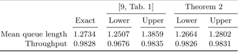
Due to length constraints, we leave the numerical assessment of Theorem 1 for future work. For an extensive numerical assessment of—the method implied by—Theorem 2, we refer the reader to [8]. We believe that in this contribution, it is more fitting to compare our method to the only existing method—at least the only one that we are aware of—that also uses lumping to provide guaranteed lower and upper bounds on limit expectations. This method was first outlined by Franceschinis and Muntz [9], and then later improved by Buchholz [3]. In order to display the benefit of their methods, they use them to determine bounds on several performance measures for a closed queueing network that consists of a single server in series with multiple parallel servers. We use the method outlined in Sect. 4.2 to also compute bounds on these performance measures, as reported in Table 1. Note that our bounds are tighter than those of [9]. We would very much like to compare our method with the improved method of [3] as well. Unfortunately, the system parameters Buchholz uses do not—as far as we can tell—correspond to the number of states and the values for the performance measures he reports in [3, Fig. 3], thus preventing us from comparing our results.
Table 1.Comparison of the bounds obtained by using Theorem 2 with those obtained by the method presented in [9, Sect. 3.2] for the closed queueing network of [9].
[9, Tab. 1] Theorem 2 Exact Lower Upper Lower Upper Mean queue length 1.2734 1.2507 1.3859 1.2664 1.2802 Throughput 0.9828 0.9676 0.9835 0.9826 0.9831
5
Conclusion
Broadly speaking, the conclusion of this contribution is that imprecise CTMCs are not only a robust uncertainty model—as they were originally intended to be—but also a useful computational tool for determining bounds on inferences for large-scale CTMCs. More concretely, the first important observation of this contribution is that lumping states in a homogeneous CTMC inevitably introduces imprecision, in the sense that we cannot exactly determine the parameters that describe the dynamics of the lumped stochastic process without also explicitly determining the original process. The second is that we can easily characterise a set of processes that definitely contains the lumped process, in the form of an imprecise CTMC. Using this imprecise CTMC, we can then determine guaranteed lower and upper bounds on marginal and limit expectations with respect to the original chain. From a practical point of view, these results are helpful in cases where state space explosion occurs: they allow us to determine guaranteed lower and upper bounds on inferences that we otherwise could not determine at all.
Regarding future work, we envision the following. For starters, a more thorough numerical assessment of the methods outlined in Sect. 4 is necessary. Furthermore, it would be of theoretical as well as practical interest to determine bounds on theconditional expectation of a lumpable function, or to consider functions that depend on the state atmultiple time points. Finally, we are developing a method to determine lower and upper bounds on limit expectations that only requires the solution of a simple linear program.
Acknowledgements
Jasper De Bock’s research was partially funded by H2020-MSCA-ITN-2016 UTOPIAE, grant agreement 722734. Furthermore, the authors are grateful to the reviewers for their constructive feedback and useful suggestions.
References
1. Anderson, W.J.: Continuous-Time Markov Chains. Springer-Verlag (1991) 2. Ball, F., Yeo, G.F.: Lumpability and marginalisability for continuous-time Markov
chains. Journal of Applied Probability30(3), 518–528 (1993)
3. Buchholz, P.: An improved method for bounding stationary measures of finite Markov processes. Performance Evaluation62(1), 349–365 (2005)
4. Burke, C.J., Rosenblatt, M.: A Markovian function of a Markov chain. The Annals of Mathematical Statistics29(4), 1112–1122 (1958)
5. De Bock, J.: The limit behaviour of imprecise continuous-time Markov chains. Journal of Nonlinear Science27(1), 159–196 (2017)
6. Erreygers, A., De Bock, J.: Imprecise continuous-time Markov chains: Efficient computational methods with guaranteed error bounds. In: Proceedings of ISIPTA’17. pp. 145–156. PMLR (2017), extended pre-print: arXiv:1702.07150
7. Erreygers, A., De Bock, J.: Computing inferences for large-scale continuous-time Markov chains by combining lumping with imprecision (2018), arXiv:1804.01020 8. Erreygers, A., Rottondi, C., Verticale, G., De Bock, J.: Imprecise Markov models
for scalable and robust performance evaluation of flexi-grid spectrum allocation policies (2018), submitted, arXiv:1801.05700
9. Franceschinis, G., Muntz, R.R.: Bounds for quasi-lumpable Markov chains. Per-formance Evaluation20(1), 223–243 (1994)
10. Ganguly, A., Petrov, T., Koeppl, H.: Markov chain aggregation and its applications to combinatorial reaction networks. Journal of Mathematical Biology69(3), 767–797 (2014)
11. Krak, T., De Bock, J., Siebes, A.: Imprecise continuous-time Markov chains. Inter-national Journal of Approximate Reasoning88, 452–528 (2017)
12. Moler, C., Van Loan, C.: Nineteen dubious ways to compute the exponential of a matrix, twenty-five years later. SIAM Review45(1), 3–49 (2003)
13. Norris, J.R.: Markov chains. Cambridge University Press (1997)
14. Rottondi, C., Erreygers, A., Verticale, G., De Bock, J.: Modelling spectrum assign-ment in a two-service flexi-grid optical link with imprecise continuous-time Markov chains. In: Proceedings of DRCN 2017. pp. 39–46. VDE Verlag (2017)
15. ˇSkulj, D.: Efficient computation of the bounds of continuous time imprecise Markov chains. Applied Mathematics and Computation250, 165–180 (2015)