A Comprehensive Study on the Estimation of Freeway Travel Time Index and the Effect of Traffic Data Quality

(1)

University of Wisconsin Milwaukee

UWM Digital Commons

Theses and Dissertations

May 2019

A Comprehensive Study on the Estimation of

Freeway Travel Time Index and the Effect of Traffic

Data Quality

Ambily Pankaj

University of Wisconsin-Milwaukee

Follow this and additional works at:https://dc.uwm.edu/etd

Part of theCivil Engineering Commons

This Thesis is brought to you for free and open access by UWM Digital Commons. It has been accepted for inclusion in Theses and Dissertations by an authorized administrator of UWM Digital Commons. For more information, please [email protected].

Recommended Citation

Pankaj, Ambily, "A Comprehensive Study on the Estimation of Freeway Travel Time Index and the Effect of Traffic Data Quality"

(2019).Theses and Dissertations. 2110.

(2)

A COMPREHENSIVE STUDY ON THE ESTIMATION

OF FREEWAY TRAVEL TIME INDEX AND THE

EFFECT OF TRAFFIC DATA QUALITY

by

Ambily Pankaj

A Thesis Submitted in

Partial Fulfillment of the

Requirements for the Degree of

Master of Science

in Engineering

at

The University of Wisconsin-Milwaukee

(3)

ii

ABSTRACT

A COMPREHENSIVE STUDY ON THE ESTIMATION OF

FREEWAY TRAVEL TIME INDEX AND THE EFFECT OF

TRAFFIC DATA QUALITY

by

Ambily Pankaj

The University of Wisconsin-Milwaukee, 2019 Under the Supervision of Professor Dr. Xiao Qin

Travel time reliability aims to quantify the variation of travel time by using the entire range of travel times for a given trip, for a selected time period over a selected horizon. A trip can occur over a segment, facility or any subset of the transportation network, for the purpose of

calculating travel time reliability. As one of the most important performance measures, travel time reliability reports the number of trips that fail or succeed according to a predetermined standard. Unreliability is usually caused by the interaction of factors that influence travel times, such as fluctuations in demand due to daily or seasonal variation, or special events, traffic control devices, traffic incidents, inclement weather, work zones, and physical capacity. These factors collectively produce travel times that can be better presented by a probability distribution.

A well-accepted measure of travel time reliability is the Travel Time Index (TTI) formulated as the ratio of travel time in the peak period to the travel time at free-flow conditions. In this thesis, the Travel Time Index values were calculated and compared from two different kinds of data sources: probe vehicles and fixed location detectors. Speed from vehicle probe data can be retrieved from the National Performance Management Research Dataset (NPMRDS) and the

(4)

iii

freeway segment speed can be calculated by dividing the segment length by the total travel time. Spot speed from fixed location detectors can be retrieved from the Wisconsin’s Archived Data Management Systems (ADMS), V-SPOC (Volume, Speed and Occupancy) which measures the speed at certain locations of a segment. The free flow speed also varies by data source. In the V-SPOC data, the posted speed limit is considered to be the free flow speed and in the NPMRDS data, the reference speed which is the 85th percentile speed of all observed sample speeds is considered to be the free flow speed.

The effect of data quality on the TTI values is also examined in the thesis. Inductive loop detectors are a major source of traffic information, but they are often criticized for generating missing and faulty data which compromise real-time traffic control, operations, and

management. There is no doubt that the quality of data will affect the accuracy of the calculation of Travel Time Index and its influence needs to be quantified. This study area was chosen to be the one that contains all different kinds road segments like basic, weaving, on ramp and off ramp segments. The result shows that the removal of invalid data improves the TTI index in the congested traffic conditions.

Lastly, a traffic simulation application, FREEVAL-RL tool, was applied to calculate the Travel Time Index. The sensitivity analysis of some important parameters used in the FREEVAL-RL Tool was performed. Calibration procedure was designed and carried out for the tool to reflect the real-world scenarios such as are Capacity Adjustment Factor, jam density and capacity drop. The outcome of the calibrated model was consistently matched to the travel time distribution in terms of mean, 50th percentile, 80th percentile, 95th percentile Travel Time Index (TTI) reported in the NPMRDS data.

(5)

iv

(6)

v To my parents, my husband and

(7)

vi

LIST OF FIGURES

Figure 3-1: Data Collection Area for V-SPOC. ... 12

Figure 3-2: Data collection Area. ... 14

Figure 3-3: Speed vs Time for 4 stations ... 18

Figure 3-4: TTI with 63mph and 55mph as FFS ... 19

Figure 3-5: TTI based on NPMRDS data. ... 20

Figure 3-6: TTI values from NPMRDS and V-SPOC data. ... 22

Figure 4-1: Speed vs Volume Diagram-Whitney Way ... 28

Figure 4-2: Speed vs Volume Diagram-Verona Road ... 28

Figure 4-3: Speed vs Volume Diagram-Seminole Hwy ... 29

Figure 4-4: Speed vs Volume Diagram-Todd Dr ... 29

Figure 4-5: Comparison of TTI for different scenarios. ... 32

Figure 4-6: Comparison between TTI values after removal of invalid data ... 33

Figure 5-1: Calibration Procedure ... 37

Figure 5-2: FD Diagram for Todd Dr. ... 42

Figure 5-3: DAF - National default values ... 45

(11)

x

LIST OF TABLES

Table 1.1: Snapshot of Recommended Reliability Measures ... 2

Table 4.1: Amount of data removed ... 30

Table 4.2: TTI values for all scenarios ... 31

Table 5.1: Estimated Capacity, % Capacity Drop and Jam Density ... 43

Table 5.2: FREEVAL-RL Output for CAF and SAF Related Scenarios ... 43

Table 5.3: FREEVAL-RL tool values ... 47

Table 5.4: Comparison of TTI values ... 48

(12)

xi

LIST OF ABBREVATIONS

ADMS Archived Data Management Subsystem or Archived Data Management System

CAF Capacity Adjustment Factor

DAF Demand Adjustment Factor

FFS Free Flow Speed

FHWA Federal Highway Authority

FSG Freeway Scenario Generator

Mph Miles per hour

NPMRDS National Performance Management Research Data Set

Pc/hr/ln Passenger Car per hour per lane

SAF Speed Adjustment Factor

TTI Travel Time Index

(13)

xii

ACKNOWLEDGEMENTS

Foremost, I would like to express my sincere gratitude to my advisor Dr. Xiao Qin for the continuous support of my master’s study and research, for his patience, motivation, enthusiasm, and immense knowledge. His guidance helped me in all the time of research and writing of this thesis. I could not have imagined having a better advisor and mentor for my master’s study.

Besides my advisor, I would like to thank the rest of my thesis committee: Dr Yue Liu and Dr. Lingqian Hu, for their encouragement, insightful comments, and hard questions.

I am truly grateful to my friend Dr. Mohammad Razaur Rahman Shaon and Md Abu Sayed for helping me out and giving extraordinary comments. I would also like to thank my friends and well-wishers who has given me constant support and encouragement throughout the course of my study.

Last but not the least I would like to thank my husband and my son for their unconditional love and support and my parents for giving me strength to pursue my study.

(14)

1

INTRODUCTION

1.1

Travel Time Reliability and Travel Time Index

Over the years the traffic congestion has been increasing significantly, according to Federal Highway Administration (FHWA) (Traffic Congestion and Reliability: Linking Solutions to Problems, 2004). According to nationwide statistics on congestion ,an average urban commuter is stuck in traffic for 34 hours per year.(“Sitting & Fuming: Traffic Congestion Statistics.,” n.d.). The growing congestion has resulted in highly unreliable information regarding estimated travel time. Performance measures based on travel time have recently been introduced to monitor existing traffic conditions and communicate with road users in an easy-to-understand manner. Travel time and its reliability are considered by the road user to be more intuitive measures of service quality than the levels of service defined in the Highway Capacity Manual (HCM) (National Research Council, 2010).

Travel time reliability predicts the number of trips that fail or succeed in accordance with a pre-determined performance standard and can be expressed through metrics such as on-time

performance or percent failure based on a target minimum speed or travel time. Drivers usually are aware of everyday congestion, and plan for it accordingly; but unexpected congestion stemming from random events such as demand variations, weather, incidents, work zones, and special events are generally unpredictable((NRC)., n.d.). Travelers also tend to remember the few bad days they spent in traffic, rather than the average time spent traveling throughout the year (“Sitting & Fuming: Traffic Congestion Statistics.,” n.d.). Hence, travel time reliability has increasingly been used to measure the extent of these delays due to non-recurrent congestion, as defined by the Federal Highway Administration (FHWA) as "the consistency or dependability in

(15)

2

travel times, as measured from day -to-day and/or across different times of the day .The most effective methods of measuring travel time reliability as proposed in different literature are 90th or 95th percentile travel times, Buffer Index and Planning Time Index(PTI).(Federal Highway Administration (FHWA)., n.d.)

Table 1.1 Snapshot of Recommended Reliability Measures

Reliability Performance Measure Definition

Core Measure

Reliability rating Percentage of trips serviced at or below

a threshold travel time index (TTI) (1.33 for freeways, 2.50 for urban streets)

Planning time index (PTI) 95th percentile TTI (95th percentile travel time divided by the free-flow travel time)

80th percentile TTI 80th percentile TTI (80th percentile

travel time divided by the free-flow travel time)

Semistandard deviation The standard deviation of travel time pegged to free-flow travel time rather than the mean travel time (variation is measured relative to free-flow travel time)

Failure or on-time measures Percentage of trips with space mean speed less than 50, 45, and/or 30 mph

Supplemental Measure

Standard deviation Usual statistical definition

Misery index (modified) The average of the highest 5% of travel times divided by the free-flow travel time

(Kittelson & Vandehey, 2016)

Table 1.1 shows the Recommended reliability measures as discussed in Highway Capacity Manual (HCM).

According to FHWA, the Travel Time Index is the ratio of the peak-period travel time to the free-flow travel time. The Planning Time Index is the ratio of the 95th percentile travel time to

(16)

3

the free-flow travel time. The measure is computed during the AM and PM peak periods as defined in the TTI, and averages across urban areas, road sections, and time periods are weighted by VMT using volume estimates. The free-flow speed is calculated as the 85th percentile of off-peak speeds, where off-off-peak is defined as Monday through Friday, 9 am to 4 pm and 7 pm to 10 pm, as well as Saturday and Sunday 6 am to 10 pm.

Travel time reliability can be calculated by using the entire range of travel times for a given trip, for a selected time over a selected horizon. The distribution of travel time of trips using a facility over an extended period represents the travel time reliability. This distribution arises from the interaction of several factors that influence travel times like recurring fluctuations in demand in time; severe weather; incidents; work zones that reduce capacity and (for longer-duration work) may also influence demand; and special events that produce temporary, intense traffic demands which may be managed in part by changes to the facility’s geometry or traffic control.

Travel time reliability analysis can be used to improve the operation, planning, prioritization, and programming of transportation system improvement projects in the following applications: long range transportation plans (LRTPs), transportation improvement programs (TIPs), corridor or area wide plans, major investment studies, congestion management, operations planning, and demand forecasting.

Wisconsin’s Archived data management systems is called V-SPOC (Volume, Speed and Occupancy). This data is mainly from fixed location detectors. National Performance

Management Research Data Set (NPMRDS) is a form of commercial GPS probe data; that is, the traffic conditions are derived from vehicles that periodically self-report speed, position, and heading with GPS electronics. Travel Time Index is calculated from both the data sources.

(17)

4

1.2

Research Goal and Objectives

This is a comprehensive study on Travel Time Reliability and Travel Time Index. It includes the determination of TTI using different types of data sources like fixed location detectors and vehicle probe data. The effects of quality of data used namely fixed location detectors, in its determination and the basic validity tests that need to performed is also discussed. Lastly, this study also compares the TTI values calculated analytically and using alternate methods of determining TTI like FREEVAL-RL tool and its calibration.

1.3

Thesis Outline

The thesis is organized as follows:

Chapter 1 introduces Travel time reliability and Travel Time index. This chapter also discusses importance of Travel time reliability as a performance measure and the research goal and objectives.

Chapter 2 discusses the literature review on travel time reliability and travel time index for the study. The review includes several papers on outlier detection and data quality. This section also includes a review on FREEVAL-RL tool and its calibration.

Chapter 3 examines the differences between two different data sources like V-SPOC and NPMRDS and how much it affects the TTI calculation. The study also briefly discusses the limitations and strengths of each.

Chapter 4 explores the effect of data quality on the TTI values. Different validity tests are conducted and the effect of data outliers in the TTI values are explored and quantified.

(18)

5

Chapter 5 discusses the calculation of TTI using the FREEVAL-RL tool. It also includes the comparison between the values obtained from the NPMRDS and V-SPOC data.

Chapter 6 summarizes the entire research. It also includes major contributions and concludes the thesis with areas of future research.

(19)

6

LITERATURE REVIEW

Travel Time Reliability is one of the performance measures in evaluating a facility, a road corridor or a road segment. Travel time reliability predicts the number of trips that fail or succeed in accordance with a pre-determined performance standard and can be expressed

through metrics such as on-time performance or percent failure based on a target minimum speed or travel time. Drivers usually are aware of everyday congestion, and plan for it accordingly; but unexpected congestion stemming from random events such as demand variations, weather, incidents, work zones, and special events are generally unpredictable. The National

Transportation Operations Coalition Performance Measurement Initiative also identified travel time reliability as key measures for operations programs.((NRC)., n.d.)

One of the earliest organizations to use reliability performance measures to describe and address urban congestion problems is the Texas Transportation Institute, which publishes its renowned annual Urban Mobility Report (Schrank, D., B. Eisele, 2012). Subsequently, various

performance measures have been proposed in the literature to quantify travel time reliability, including 95th percentile travel time, travel time index (TTI), planning time index (PTI), and buffer time index (BTI). The foundation study performed by Cambridge Systematics, Inc in Analytic Procedures for Determining the Impacts of Reliability Mitigation Strategies recommended several reliability measures derived from travel time distributions, and it also explained the data needs for estimating prediction models and developed travel time reliability prediction models. The analytical procedures provide tangible solutions to incorporate travel time variations into transportation planning, operations, simulation, and evaluations.((NRC)., n.d.) .

(20)

7

National Research Council emphasizes that reliability measures should be derived from the distribution of travel time from a minimum of six months of traffic data. The available data sources play a significant role in travel time computation. Traditional Intelligent Transportation Systems (ITS) detectors such as loop, radar detectors cannot measure travel time directly since they measure speed and volume at specific points of the roadway. The “floating car” test vehicle has been used previously as a method to collect travel time data, but this method is costly and may have limited coverage both spatially and temporally. It would be desirable to have travel time data that are widespread, accurate, reliable, cost competitive, anonymous to data collector and less reliant on agency infrastructure. The National Performance Management Research Data Set (NPMRDS) is one of the few data sources that meet all the requirements.(Rafferty, P., 2014)

The National Performance Management Research Data Set (NPMRDS) was procured by the FHWA Office of Operations in 2013. The datasets cover the complete National Highway System, and data sources are based on cellphone apps and in-vehicle navigation systems. NPMRDS differs from commercially available data feeds in that FHWA specified that no smoothing, outlier detection, or imputation of traffic data be performed. As a result, NPMRDS contains unique characteristics for statistical distribution of reported travel times. These are characteristics such that traditional processing techniques are ineffective in obtaining accurate performance measures. Kaushik K et al. proposes a method for handling the challenges posed by NPMRDS and computing meaningful performance measures from it. The paper discusses the challenges in processing NPMRDS data and defines a method for overcoming the challenges. The paper compares the results from the proposed method with traffic data from commercial probe data sources and a reference reidentification data source at two case study locations. The

(21)

8

case studies indicate that this paper successfully shows the ability to capture performance measures from NPMRDS more accurately with techniques originally developed to accurately reflect travel time and travel time reliability on interrupted-flow facilities. (Kaushik, K., Sharifi, E., & Young, 2015).

The travel time data usually have outliers. The outlier detection algorithm is used to detect extreme values that result from sampling bias. Haghani et al.,2010 introduced moving average speed based upper and lower bound to avoid arbitrary fixed bound outlier filtering methods. Dion and Rakha ,2006 incorporated few simple alterations in the adaptive method which they proposed. (Dion, F. & Rakha, 2006)The main alteration is expanding the data validity window when three consecutive observations fall either above or below the window. This adjustment helps to capture the changes in travel time trend, though it compromises on accuracy of travel time estimation. In most cases, the sophistication of filtering algorithms led to a certain level of complexity in real-time applications. So, a simplified version of these algorithms is preferred.

Kalman Filter, an optimal recursive data processing algorithm, has been widely used with various modifications (e.g. adaptive KF(Guo, J., Huang, W. Williams, 2014) and extended KF (Liu, H., Van Zuylen, H., Van Lint, H. ,Salmons, 2006)in several studies including those on travel time prediction. KF incorporates all information that can be provided and processes all available measurements to estimate the current value of the variables of interest (Maybeck, 1990). The KF method has two components: process/system/state-space and

measurement/observation. Based on the paper by Hasan M. Moonam et al. the k-NN, LSBoost and KF algorithms were used to predict Departure Travel Time (DTT) and thus assist motorists

(22)

9

by providing a more accurate and reliable travel time.(H.M. Moonam, X. Qin, 2018) Overall, KF outperformed other two methods.

Over the years, several validity tests have been proposed and applied to flag invalid traffic records and assess system-wide data quality for archived traffic data. Typical QA/QC procedures can be classified into two categories: 1) univariate and multivariate range checks, which validate a single traffic variable or a combination of traffic variables (e.g., traffic volume, speed, and occupancy) against predetermined thresholds (e.g., the minimum, maximum and/or appropriate range of values); and 2) temporal consistency based on the comparison between historical trends and patterns and spatial consistency checks which evaluate the consistency of traffic

observations made from nearby detector locations (e.g., upstream, downstream locations or adjacent lanes if performed on lane-specific basis). Additionally, diagnostics based on detailed sensor signal outputs like the sensor on-/off-time have been developed to identify detector errors such as the sensitivity issue, pulse-breakup errors, and chronic splash over errors.

According to Zhi Chen et al. basic validity tests should be identified to maintain minimum data quality. The candidate validity tests should be identified based on user’s preference and

programming complexity. Rules of candidate validity tests can be established using the rule-based method and the data-driven method. Candidate validity tests should be evaluated regarding their effectiveness in flagging questionable data. Lastly, if all tests will not be implemented, a subset of candidate validity tests that collectively provide satisfactory data quality can be determined for implementation.(Qin, Chen, & Cheng, 2018).

The increasingly accessible travel time data has led to advancements in methodologies for analyzing and predicting freeway services, as reflected in the HCM. The project Incorporating

(23)

10

Travel-Time Reliability into the Highway Capacity Manual developed new analytical procedure for reliability assessment and the implementation tool FREEVAL-RL based on the HCM freeway and urban street facility procedures and computational engines.(Kittelson & Vandehey, 2016) .Calibration is required for any tools or models that want to be considered for a real-world application because any analysis that uses the HCM methodology depends on an accurate

representation of daily recurring congestion conditions. Calibrating the parameters in a model is a complex task, as each model may require a large number of input variables from the field data. Moreover, the availability, accessibility and quality of the field data challenge the success of model calibration. The existing references on model calibration are very limited, which presents a major barrier to agencies who want to apply the methodology.

Following the principles of traffic flow theory, the calibration procedure is supported by data-driven sensitivity analysis to determine the relative importance of input variables pertinent to their influence on travel time distribution. The study illustrates the calibration was successfully performed to match the travel time distribution in terms of mean, 50th percentile, 80th percentile, 95th percentile Travel Time Index (TTI) reported in the National Performance Management Research Data Set (NPMRDS).(Shaon, Mohammad Razaur Rahman, Xiao Qin, 2018)

(24)

11

MEASUREMENT OF TRAVEL TIME INDEX

3.1

Archived Data Management Systems (ADMS) Data

Informed travel decisions rely on intelligent transportation management systems that are

supported by large-scale traffic surveillance data. Inductive loop detectors are a major source of traffic information, but they are often criticized for generating missing and faulty data which compromise real-time traffic control, operations, and management. Archived loop detector data are used for off-line analytical purposes, such as transportation planning, congestion monitoring, and performance measures. Archived data management systems (ADMS) have been used

extensively to store historical traffic data collected from traffic sensors such as loop detectors and microwave detectors. Traffic data are essential for off-line analytics such as transportation planning, congestion monitoring, and performance measures. Wisconsin’s Archived data management systems is called V-SPOC (Volume, Speed and Occupancy).

3.1.1

Data Collection Area for V-SPOC

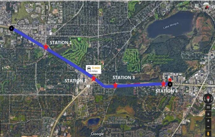
The proposed data collection area was tested on a study site located in Madison, Wisconsin. The study area selected is a segment on US 12 EB from Whitney Way to Todd Dr containing 4 Count stations. The geometric configuration of the study corridor is collected from Google Map and MetaManger, Wisconsin’s highway inventory database. The Meta-Manager system database contains a geographically integrated set of corporate databases for the Wisconsin State Trunk Highway Network. The corridor is a suitable study area because all segment types are included: Basic, On-ramp, Off-ramp, and Weaving (Eads & Cmt, 2011)

(25)

12

Figure 3-1 Data Collection Area for V-SPOC.

Figure 3-1 shows the location of the study area selected. The distance between stations are also measured.

The distance between Station 1 and Station 2 is 1.24 miles, the distance between Station 2 and Station 3 is 0.5 miles and the distance between Station 3 and Station 4 is 1.05 miles.

3.1.2

Traffic Data Description

The selected segment is instrumented with four detector stations with dual loop detectors that continuously collect traffic volume, speed and occupancy for each lane at 30 second time

interval. The data is collected from WisTransportal system for every 15 minutes for the 4 stations for the year of 2014.The data is collected only for weekdays, Tuesday to Thursday. Rest of the weekdays, weekends and holidays are excluded as the traffic pattern is different during this time.

(26)

13

3.2

NPMRDS Data

In 2013, FHWA Office of operations procured the National Management Research Data Set, which initially served as research data set for sponsored programs. The rights to use this data set were secured for state departments of transportation and metropolitan planning organization in anticipation of performance measure requirements of the Moving Ahead for Progress in the 21st Century Act. NPMRDS is a form of commercial GPS probe data; that is, the traffic conditions are derived from vehicles that periodically self-report speed, position, and heading with GPS electronics. This data set differs from commercially available data feeds in that FHWA specified that no smoothing, outlier detection, or imputation of traffic data be performed. As a result, NPMRDS contains unique characteristics for statistical distribution of reported travel times. These are characteristics such that traditional processing techniques are ineffective in obtaining accurate performance measures(Kaushik, K., Sharifi, E., & Young, 2015). Vehicle probe data is different from other speed/travel time data such as those collected from location-fixed traffic detectors. NPMRDS gives us the Space mean speed. Space Mean speed ensures that there is an equivalent travel time along the same road segment and it can be exclusively calculated by the speed and the segment length.

(27)

14

3.2.1

Data Collection Area for NPMRDS

The study area selected is a segment on US 12 EB from Grand Canyon Dr (a little before Whitney Way) to a little distance after Todd Dr. The geometric configuration of the study corridor is collected from Google Map and MetaManger, Wisconsin’s highway inventory database. The Meta-Manager system database contains a geographically integrated set of corporate databases for the Wisconsin State Trunk Highway Network.

Figure 3-2:Data collection Area.

Figure 3-2 shows the location of the data collection area selected. The distance between stations are also measured.

(28)

15

3.2.2

Traffic Data Description

The NPMRDS data were collected in 15-minute bins from 24 Traffic Message Channels (TMC). The geographic information used for TMC is distributed in the form of location code lists. TMC segment are important as it contains both their location codes but is also requires the location codes of the previous and the next segment in this chain. While loop detectors, have just one location and it gives continuous data which is collected throughout the year. The TMC segments and V-SPOC data segments are different length but the total segment length of 3.8 miles is the same.

The data is collected from NPMRDS system for every 15 minutes for the year of 2014.The data is collected only for weekdays, Tuesdays to Thursdays from 2PM to 7PM. Rest of the weekdays, weekends and holidays are excluded as the traffic pattern is different during this time. Vehicle probe data is different from other speed/travel time data such as those collected from location-fixed traffic detectors. NPMRDS gives us the Space mean speed. Space Mean speed ensures that there is an equivalent travel time along the same road segment and it can be exclusively

calculated by the speed and the segment length.(Preliminary Recommendations on Probe Data - Draft v1, n.d.)

(29)

16

3.3

Methodology

The TTI is calculated for PM Peak. The PM peak is determined by the looking at the speed at each hour for all the stations. The raw data from both V-SPOC and NPMRDS are both

amalgamated with same frequency of 15 minutes. The average segment speed is calculated using segment length as weight.

The x percentile Travel Time Index is calculated by the formula given below.

= =

The travel time index is calculated for both data sources using both speed limit and reference speed as free flow speed. Reference Speed is the calculated “free flow” mean speed for the roadway segment in miles per hour (capped at 65 miles per hour). This attribute is calculated based upon the 85th-percentile point of the observed speeds on that segment for all time periods, which establishes a reliable proxy for the speed of traffic at free-flow for that segment.(INRIX Inc., n.d.).Reference speed is directly available from the NPMRDS data. The same reference speed is used as Free Flow speed in both TTI calculation from V-SPOC and NPMRDS data.

For V-SPOC, the data collected include speed data from 4 stations. The speed of the whole segment needs to be calculated. The speed of the segment is calculated by.

= (L1 V1+ L2 V2+ L3 V3+ L4 V4)

Where L1, L2, L3 and L4 are lengths of segments whose speed is V1, V2, V3 and V4 respectively.

(30)

17

apply the spot mean speed to a longer section, the spot mean speed is assumed to be the same for half section length upstream and half section length downstream of the detector.

In case of NPMRDS, the data collected include speed data from 8 segments. So, the speed of the whole segment needs to be calculated. The speed of the segment is calculated by.

= (L1 V1+ L2 V2+ L3 V3+ L4 V4+ L5 V5+ L6 V6+ L7 V7+ L8 V8)

Where L1, L2, L3, L4, L5, L6, L7 and L8 are lengths of segments whose speed is V1, V2, V3, V4, V5,

(31)

18

3.4

Data Analysis and Discussion of Result

3.4.1

V-SPOC Data Analysis

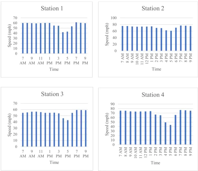
The PM Peak is obtained by looking at the hourly speed at four Stations.

Figure 3-3:Speed vs Time for 4 stations

From the above graph the PM peak is considered from 3PM to 6 PM. But the data is taken from 2PM to 7PM including the one hour of free flow condition before and after the PM Peak hour.

Then the missing data is removed and then the segment speed is calculated. The average segment speed is calculated using segment length as weight.

0 10 20 30 40 50 60 70 7 AM 9 AM 11 AM 1 PM 3 PM 5 PM 7 PM 9 PM S p ee d ( m p h ) Time

Station 1

0 20 40 60 80 100 7 A M 8 A M 9 A M 1 0 A M 1 1 A M 1 2 P M 1 P M 2 P M 3 P M 4 P M 5 P M 6 P M 7 P M 8 P M 9 P M S p ee d ( m p h ) Time

Station 2

0 10 20 30 40 50 60 70 7 AM 9 AM 11 AM 1 PM 3 PM 5 PM 7 PM 9 PM S p ee d ( m p h ) Time

Station 3

0 10 20 30 40 50 60 70 80 90 7 A M 8 A M 9 A M 1 0 A M 1 1 A M 1 2 P M 1 P M 2 P M 3 P M 4 P M 5 P M 6 P M 7 P M 8 P M 9 P M S p ee d ( m p h ) Time

Station 4

(32)

19

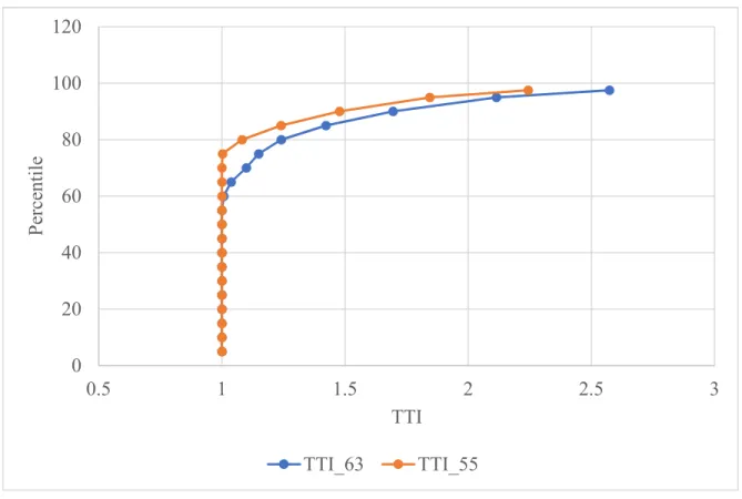
For the purpose of comparison, the TTI is calculated in two scenarios, i.e. with Speed limit of 55mph as the free flow speed and reference speed of 63 mph as Free Flow Speed. Note that the reference speed for the segment is obtained from the NPMRDS data set of the study area.

Figure 3-4: TTI with 63mph and 55mph as FFS

Error! Reference source not found.Figure 3-4 shows TTI values based on both 55mph and 63mph as free flow speed. As we are interested in TTI in congested regime, the TTI values below 1 which implies uncongested regime are converted to 1. The shapes of the two curves are similar with the values diverging from the 65th percentile TTI values. Since the reference speed of 63 mph is greater than that of the speed limit of 55 mph, the congested regime is displayed to begin earlier. The 97.5th percentile TTI with 63 mph as FFS is 2.57 while for 55 mph as speed

0 20 40 60 80 100 120 0.5 1 1.5 2 2.5 3 P er ce nt il e TTI TTI_63 TTI_55

(33)

20

limit is about 2.24. The range of TTI values is higher for 63mph as FFS than the speed limit of 55mph as FFS.

3.4.2

NPMRDS data Analysis

The data is collected from the NPMRDS data set for the PM peak for 2PM to 7PM (as calculated from the V-SPOC data) for weekdays from Tuesdays to Thursdays. The missing data is removed and then the segment speed is calculated. The records having missing data is removed in order to give a plausible TTI values. The upper limit value of Travel Time Index and Planning Time Index tends to decrease as the segment length increases (Preliminary Recommendations on Probe Data - Draft v1, n.d.). This gives biased results, likely higher than what they should be. So, the average segment speed is calculated with segment length as weight. Similarly, the TTI is calculated in two scenarios, i.e. with Speed limit of 55mph and reference speed of 63 mph which is available in the data as Free Flow Speed and the results are presented in Figure 3-5.

(34)

21

Figure 3-5:TTI based on NPMRDS data.

Figure 3-5 shows the TTI values when reference speed and speed limit is considered as free flow speed. The TTI_63 curve is shifted to the right of TTI_55 curve. As reference speed is the 85th

percentile speed of all the time periods. From this graph we can understand that the congestion regime started before started before 2PM and lasts more too. Therefore , the whole TTI curve has been shifted to the right. The difference between both the values remain approximately constant about 13% all throughout the curve. This figure above is similar to Figure 3-4 with TTI values with 63 mph as FFS having higher TTI values than that of TTI values with speed limit as FFS. This implies that the congestion condition is more severe and begins earlier than the study period. 0 10 20 30 40 50 60 70 80 90 100 0.5 1 1.5 2 P er ce nt il e TTI TTI_63 TTI_55

(35)

22

3.4.3

Discussion

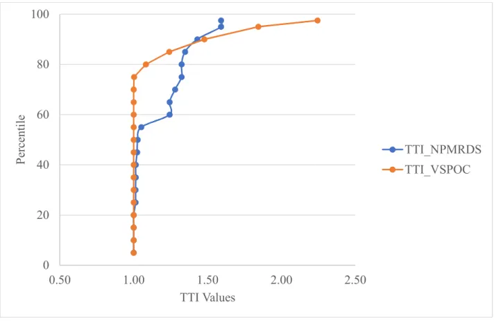
The TTI values with both Reference speed (TTI_63) and speed limit (TTI_55) as free flow speed are calculated from both NPMRDS and V-SPOC data. The TTI values obtained from both NPMRDS and V-SPOC with speed limit of 55mph as FFS are given below.

Figure 3-6:TTI values from NPMRDS and V-SPOC data.

The TTI values from both NPMRDS and VPOC are almost similar till about 60th percentile TTI and then these curves diverge to converge at 90th percentile TTI. The Planning Index (95th Percentile TTI) and Misery Index (97.5th Percentile TTI) of V-SPOC data is much higher than the NPMRDS data. The shape of two curves are completely different. While the TTI curve for data from V-SPOC is smooth, the curve from NPMRDS is not. This is due to the type of data. It is known that NPMRDS data is sample data and V-SPOC is the actual population data. But

0 20 40 60 80 100 0.50 1.00 1.50 2.00 2.50 P er ce nt il e TTI Values TTI_NPMRDS TTI_VSPOC

(36)

23

during congested regime the amount of data increases as the number of probe cars increases, hence making the distributions much closer to the actual data.

The NPMRDS data gives the travel time, speed and reference speed. However, the NPMRDS data set does not give information about the volume and occupancy, thus making some

calculations difficult, like using FREEVAL-RL tool (a tool to calculate reliability based on HCM methodologies) for improvement projects etc.

The NPMRDS data is more accurate as vehicle probe data is more reliable than fixed location detectors which gives error due to faulty detectors. The quality of data from V-SPOC is not that good as there not much comprehensive validity tests. Data errors due faulty detectors, missing data and presence of outliers affect the TTI values. So, a data quality check is necessary and questionable data need to be removed. Chapter 4 discusses the data quality check necessary to calculate the TTI more accurately.

(37)

24

EFFECTS OF DATA QUALITY ON TRAVEL

TIME INDEX

4.1

V-SPOC Data Quality

In Wisconsin, V-SPOC satisfies vital needs of the operations, planning, and research purposes. V-SPOC receives and stores raw detector data originated as a nightly extract from WisDOT Statewide Traffic Operation Center (STOC). Each extract contains over 5 million 1-minute detector data records. In the raw data, each record has: 1) timestamp, 2) detector id, 3) vehicle count, 4) average speed and 5) average occupancy. The current V-SPOC includes archived data validity tests with 5-minute loop detector data. These validity tests detect faulty data in a two-step process: a) each 5-minute record is tested against a series of predefined validity criteria from volume and speed health to occupancy health, and imperfect records are flagged as positive; and b) the flags are aggregated according to the selection of the time, area, and units. In spite of the built-in data quality flags, traffic data quality and reliability continue to be in question for WisDOT’s Transportation Systems Management & Operations (TSM&O) activities.

Many important validity test criteria – some of which have already been tested and deployed at other state DOTs and have shown various levels of success – are currently not available in V-SPOC. Therefore, the data quality in V-SPOC may be substantially benefited from

(38)

25

4.2

Methodology

The raw data is the data collected from the V-SPOC data using the WisTransportal Website. In this study 11 validity tests are conducted.

4.2.1

Basic Data Validity Tests

The basic validity tests that are conducted are:

• Test_1: Missing Data Check: If Volume, speed or occupancy is missing then the data is considered invalid.

• Test_2: Minimum Volume is 0: If Volume is less than zero, then the data is considered invalid.

• Test_3: Max. Volume is 750@ 15 min: If the volume is greater than 750 vehicles per lane every 15 mins, then data is considered invalid.

• Test_4: Max. occupancy<100%: If the occupancy is greater than 100 percent, then the data is considered invalid.

• Test_5: Max. speed<85mph: If the speed is greater than 85 mph, then the data is considered invalid.

Alternative Multi-variate checks are performed.

• Test_6: Positive volume or occupancy with no speed: If speed is zero and if the volume or occupancy is greater than zero, then the data is invalid.

• Test_7: Positive speed or occupancy with no volume: If volume is zero and if the speed or occupancy is greater than zero, then the data is invalid.

(39)

26

• Test_8: Positive speed or volume with no occupancy: If occupancy is zero and if the speed or volume is greater than zero, then the data is invalid

4.2.2

Advanced Data Validity Tests

• Test_9: Infeasible AVEL uses volume, speed and occupancy: If the Average Effective Vehicle Length (AEVL) derived based on all three variables, volume, speed, and occupancy, is valid. The equation of AEVL is as follows:

( / ℎ) =#$%%& ('(/))∗ + ,-+ ./∗011$2314∗5% 789:'% (;%)/)) = #$%%& ('(/))∗011$2314 789:'% (;%)/)) ∗ (5280/100)

The AEVL only applies to traffic records with positive values in all three variables. A valid range is 9 < < 60 as proposed in Zhi Chen et al.(Qin et al., 2018)

4.2.3

Data Outlier Detection

The outlier is an observation that are far removed from the mass of data. These outliers may not be caused by data errors but by real world scenarios such as accidents, work zones or special events while erroneous data is mainly caused by detector errors. The outliers from speed value is removed the outliers are identified from the speed vs volume diagrams for each station.

The x percentile Travel Time Index is calculated by the formula given below.

D%=

D% EF%% E98G

Misery Index is calculated using the formula given below

H I = JK.M%

(40)

27 Travel Time Index is calculated for three scenarios:

• Scenario 1: The raw unfiltered data.

• Scenario 2: With Basic Validity tests done.

• Scenario 3: With Advanced Validity test and outliers removed

The speed of the segment is calculated by Total distance divided by Total travel time. The TTI is calculated for PM Peak. The PM peak is determined by the looking at the speed at each hour for all the four stations.

4.3

Data Analysis and Discussion of Results

As given in part A, the PM peak is determined to be from 2PM to 7PM.Then the validity tests are done on the data set from WisTransportal. The data set is analyzed for two scenarios.

Scenario 1: In this Scenario, the data used is not filtered, raw data. The blanks and data where speed=0 is removed to calculate TTI correctly.

Scenario 2: The basic validity tests and multivariate tests are done, and invalid data has been removed. The tests 1 to 8 are done and invalid data are removed. The blanks and data where speed=0 is removed to calculate TTI.

Scenario 3: The basic validity tests and multivariate tests are done, and invalid data has been removed. The tests 1 to 8 are done and invalid data are removed. Then the advanced validity test is done (Test_9). Then the outliers are removed using the speed vs volume diagram. The blanks and data where speed=0 is removed to calculate TTI.

The figures below show the speed vs volume diagram in each detector station. The outlier data from each detector station were removed.

(41)

28

Figure 4-1:Speed vs Volume Diagram-Whitney Way

Figure 4-2:Speed vs Volume Diagram-Verona Road 0 10 20 30 40 50 60 70 80 90 0 100 200 300 400 500 S p ee d Volume Whitney Way 0 10 20 30 40 50 60 70 80 90 0 100 200 300 400 S p ee d Volume

Verona Rd

(42)

29

Figure 4-3:Speed vs Volume Diagram-Seminole Hwy

Figure 4-4:Speed vs Volume Diagram-Todd Dr 0 10 20 30 40 50 60 70 0 100 200 300 400 500 S p ee d Volume

Seminole Hwy

0 10 20 30 40 50 60 70 80 90 0 100 200 300 400 500 600 S p ee d Volume Todd dr

(43)

30

Though the amount of data removed are not huge hardly 1% of the total data. But the effects of its removal in TTI values like Misery Index is high.

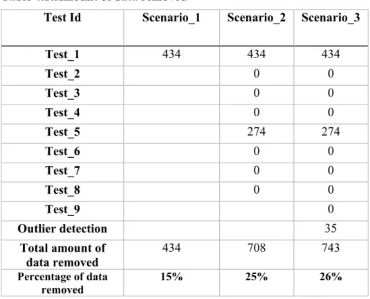
Table 4.1:Amount of data removed

Test Id Scenario_1 Scenario_2 Scenario_3

Test_1 434 434 434 Test_2 0 0 Test_3 0 0 Test_4 0 0 Test_5 274 274 Test_6 0 0 Test_7 0 0 Test_8 0 0 Test_9 0 Outlier detection 35 Total amount of data removed 434 708 743 Percentage of data removed 15% 25% 26%

Table 4.1 shows the amount of data removed in each scenario. With the validity tests the amount of data removed is almost 25% and including the outliers is 26%.

(44)

31

Table 4.2:TTI values for all scenarios

Percentile Scenario 1 Scenario 2 Scenario 3

5 1 1 1 10 1 1 1 15 1 1 1 20 1 1 1 25 1 1 1 30 1 1 1 35 1 1 1 40 1 1 1 45 1 1 1 50 1 1 1 55 1 1 1 60 1 1 1 65 1 1 1 70 1 1 1 75 1 1 1 80 1.04 1.01 1.00 85 1.18 1.07 1.06 90 1.41 1.21 1.16 95 1.75 1.53 1.43 97.5 2.22 1.95 1.64 99 2.97 2.97 1.99

(45)

32

4.3.1

Comparison

The figure below gives the comparison between the two TTI values for different scenarios.

Figure 4-5:Comparison of TTI for different scenarios.

The data quality of the V-SPOC data affects the 80th Percentile TTI onwards. The Misery Index and Planning Index of Scenario 1 is higher than Scenario 2 and Scenario 3. This implies that with data quality the Travel index decreases giving us more accurate representation of the real-world scenario. Even though, the amount of data removed is significantly smaller, TTI does vary when outliers are removed. The TTI of the road segment improves when this data is removed. But as we are interested in Planning Time Index and Misery Index reduction of these TTI values will underestimate the Travel time reliability and congestion. The variation of Misery Index between Scenario 2 and Scenario 3 are about 16%. Outliers might be caused due to accidents or some

70 75 80 85 90 95 100 0.8 1 1.2 1.4 1.6 1.8 2 2.2 2.4 2.6 2.8 3 3.2 P e rc e n ti le TTI

Comaprison of TTI

(46)

33

road conditions and not due to error in the data. No definite cause for these outliers can be deduced from the data from V-SPOC. Hence these outliers might represent the real-world data and not just data errors. In this study the outliers removed were compared with NPMRDS data source. The data during this time fame does not reflect the data in NPMRDS. So, these outliers are removed in Scenario 3.Although, NPMRDS being sample data need not represent these data accurately .

Figure 4-6:Comparison between TTI values after removal of invalid data

Figure 4-6 shows the comparison between TTI values from V-SPOC and NPMRDS data. While the shape of the curves remains the same as before. The Planning Index and Misery Index are closer together. The removal of data errors has actually improved the TTI values in the congested regime. 0 20 40 60 80 100 120 0.8 0.9 1 1.1 1.2 1.3 1.4 1.5 1.6 1.7 TTI_VSPOC TTI_NPMRDS

(47)

34

The change in TTI values depend on the dispersion of the data removed. If more data is removed from congested regime, i.e. if the data removed is skewed to the congested regime then TTI values are impacted more. But if more data is removed from uncongested region then the impact on TTI values are lesser.

In both Chapter 3 and Chapter 4 the TTI is calculated from the raw data available for existing conditions. But for improvement projects where such speed data is not available this method cannot be used. A tool called FREEVAL-RL was developed based on HCM methodologies which calculate the reliability performance measures. Chapter 5 discusses this tool and how to calibrate this tool for real-world analysis.

(48)

35

CALCULATION OF TTI USING FREEVAL-RL

5.1

FREEVAL-RL

The increasingly accessible travel time data has led to advancements in methodologies for analyzing and predicting freeway services. Reliability has become one of the most important performance measures. Based on HCM freeway and urban street facility procedures and computational engines, the SHRP 2 L08 project Incorporating Travel-Time Reliability into the Highway Capacity Manual developed new analytical procedure for reliability assessment and the implementation tool FREEVAL-RL and also developed two draft chapters for inclusion in a future version of the HCM (Kittelson & Vandehey, 2016).For real-world application ,a tool or model requires calibration because any analysis that uses the HCM methodology depends on an accurate representation of daily recurring congestion conditions. Calibrating the parameters in a model is a complex task, as each model may require many input variables from the field data. Moreover, the availability, accessibility and quality of the field data challenge the success of model calibration. The existing references on model calibration are very limited, which presents a major barrier to agencies who want to apply the methodology.

5.2

Calibrating FREEVAL-RL

The freeway analysis calibration framework, based on the sixth edition of HCM, includes:

Step 1: gather input data (facility geometry, Free Flow Speed, Demand),

Step 2: calibrate free flow speed (FFS),

(49)

36 Step 4: calibrate facility demand level,

Step 5: validate, and if the validation results do not meet the predetermined thresholds, the procedure loops back to Step 2 and new iteration begins.

FREEVAL-RL computational engine is a combination of FREEVAL (HCM 2010) and a scenario generator for estimating reliability performance measures. The scenario generator generates operational scenarios based on sources of non-recurrent congestion such as incidents, weather events, work zones etc. In this section, the principle of the HCM freeway analysis calibration is followed, but the procedures are expanded to account for the complexity of travel time under the non-recurrent congestion.

FREEVAL uses traffic flow model parameters in its assessment of traffic conditions, mostly for recurring congestion effects. The user of the tool need not define all the traffic flow parameters. The tool also provides national default values for traffic flow parameters, such as jam density, capacity drop during queue dissipation etc. But these national default values need not always represent the operational characteristics of the study corridor. Thus, it is recommended to calibrate the tool with local data when available.

Before calibrating FREEVAL-RL, it is important to assess the data items available to run the computational model and their effects on reliability performance measures. Sensitivity analysis should be performed during the calibration process to assess the influence of these parameters on performance measures if no prior knowledge or established relationship occurs. This analysis is required for a tool like FREEVAL-RL in which the field measurements for all the required parameters are not available or not in good quality. The sensitivity analysis provides an insight into which parameters need to be calibrated. Based on the paper by Shaon, Mohammad Razaur

(50)

37

Rahman, Xiao Qin et al. the recommends a step by step procedure in calibrating the FREEVAL-RL tool as shown in Figure 5-1.

(51)

38

According to the above given calibration method, the following steps were followed to arrive at the following cases.

Step 1: Execute the model with selected traffic flow parameters for the base condition with National default values. Check whether the results match with observed travel time distribution from field under same operating condition.

Run the FREEVAL-RL tool with site-specific roadway geometry and traffic demand. National default values provided in tool is used for all other parameters. This provides the base case scenario from which we need to calibrate.

Step 2: Asses the site-specific data availability and quality.

The specific data availability and quality assessment need to be done. Sometimes the site-specific data maybe available but it will not be accurate. If the data is not available or accurate then national default values are used.

Step 3: Replace all the default values with site specific values.

After a thorough assessment of available local data items, default traffic flow parameters need to be replaced with site specific values like jam density, capacity drop, demand multiplier, incident rate, duration and std. deviation. To obtain the site-specific traffic flow model parameters, the flow-density curve needs to be calibrated from the field data. The speed-flow curve is also called fundamental diagram (FD) which is an empirical curve relating observed densities to observed flows at a particular point on the road. Most macroscopic models of vehicular traffic make use of the FD because it provides a direct mapping from density to flow, including FREEVAL.

(52)

39

Step 4: Use CAF and SAF to calibrate base capacity and FFS

Although the capacity for each segment can be estimated using HCM method, the FREEVAL module allows the user to use Capacity Adjustment Factor (CAF) and Speed Adjustment Factor (SAF) to adjust the variation in estimated capacity and free flow speed due to driver factors. The FREEVAL tool provides flexibility that allows the user to use CAF which can be defined for each segment at each time slice within analysis time period to adjust the capacity of the study corridor. The SAF is used to model free-flow to reduce the impacts of scenarios causing non-recurrent congestion. Hence, the SAF should be used to adjust base FFS for effects of different scenarios rather than calibrate the base free-flow speed for a freeway segment. Use CAF or SAF or both to calibrate base scenario. Check whether the TTI outputs from FREEVAL-RL match with observed travel time distribution for mean, 50th percentile and 80th percentile.

Step 5: Conduct the sensitivity analysis for the input parameters and calibrate the input parameters based on the sensitivity analysis.

Then, if the mean, 50th percentile and 80th percentile TTI outputs from FREEVAL-RL does not match with field conditions, a sensitivity analysis need to be conducted to evaluate their

sensitivity with reliability performance measures. FREEVAL module also allows the user to input capacity drop, a traffic flow phenomenon that can be observed from real-time traffic data. Previous studies have shown that there is a difference in capacity when a queue is built up versus when a queue is dissipated. (Nisbet, J., D. Bremmer,2014) The capacity is normally higher when the traffic queue builds up. The FREEVAL-RL tool does not have the ability to model capacity drop from the input data but allows the user to input a capacity drop value between 0 to 10% with a national default value of 5%. Similar to capacity drop, the FREEVAL module allows the

(53)

40

user to select a jam density for the study corridor between 130 to 360 passenger cars per mile per lane (pc /mi /ln). The national default value for jam density is provided as 190 pc /mi /ln. The FREEVAL-RL only allows users to enter a certain jam density value throughout the study period. When the tool is unable to reflect the actual capacity drop, the user may need to calibrate the capacity level by using CAF or SAF or both to avoid the underestimation of the congestion. The mean, 50th percentile and 80th percentile TTI values can be adjusted by varying CAF and SAF along with other traffic flow parameters defined in Step 3.

Step 6: Conduct the sensitivity analysis for Freeway Scenario Generator (FSG) input parameters.

If the 95th percentile and the misery index outputs from FREEVAL-RL are different, the

parameters in the freeway scenario generator (FSG) need to be changed. The incident events are rare and may cause worst non-recurrent congestion. Hadi et al. noted that incident input

parameters can significantly influence the 95th percentile of TTI outputs from FREEVAL-RL computational engine (Ramirez, Hu, Xiao, Shabanian, & Hadi, 2015). Based on sensitivity analysis results, the input parameters in FSG should be adjusted to match 95th percentile and misery index (97.5th percentile) outputs from FREEVAL-RL with field condition.

These steps are used for data rich environment where all major input parameters are available and could be verified. This provides a guideline to calibrate the tool.

5.3

Case Study

The proposed calibration framework was tested in the same study area as in Chapter 3 and Chapter 4. The selection of study corridor plays an important role in obtaining reliable outputs from the FREEVAL-RL. The selected study corridor in FREEVAL-RL should start and end with

(54)

41

a basic segment and should not operate at LOS F. The study area chosen is 3.8 miles long has 9 segments which begins and ends with a basic segment, including 5 basic segments,2 weaving segments, 1 on-ramp segment and 1 off-ramp segment. According to FREEVAL-RL

requirements, it is safe to choose a time period where the starting and ending time slice operates at or near free-flow speed. So, a time period of 2PM to 7PM was chosen for the analysis, because the congestion usually begins around 3PM and ends by 6PM.

The selected corridor was equipped with dual loop detectors that collect traffic volume, speed, and occupancy for each lane at 30-second time intervals. The data is stored in an Oracle database and is accessible via the V-SPOC traffic detector database. An FD diagram was calibrated by fitting a fundamental traffic flow model to the volume and density measurements for the site selected in this study. The traffic detector data were collected in 5-minute bins along the mainline of the study corridor between the months of March and September from V-SPOC database. The FD diagram was calibrated only for mainline traffic detector locations within the study corridor. The FD plot for a mainline detector location at Todd Drive is shown in

(55)

42

Figure 5-2:FD Diagram for Todd Dr.

Figure 5-2 shows that the flow builds up till capacity until queue starts. Once the queue starts building up after achieving capacity the capacity drop can be observed. After the capacity drop, then the queue starts to dissipate. Methodologies for measuring capacity, jam density, and

capacity drop from field data have been explored in the literature. Estimating a best-fit regression line in the congested traffic condition can provide the jam density. The estimated capacity, percent capacity drop, and jam density obtained from calibrating the FD diagrams are provided

(56)

43

in. The calibrated capacity drop, and jam density can be used to replicate the congested traffic conditions that occurred on the study corridor.

Table 5.1:Estimated Capacity, % Capacity Drop and Jam Density Location Capacity (pc/hr/ln) Dropped Capacity (pc/mile/ln) % Capacity Drop Jam Density (pc/mi/ln) Whitney Way 2054 1656 19.38% 233.0 Verona Rd 2312 1890 18.25% 222.0 Seminole Hwy 2506 1992 20.51% 202.5 Todd Dr. 2195 1741 20.68% 216.7

Table 5.1 shows that the capacity drops ranges between 18 and 20 percent on the study area. Since the FREEVAL-RL allows only a maximum of 10 percent drop, so the maximum capacity drop was used in this case. The average jam density on the study corridor was 219 pc/mi/ln. The literature suggests replacing national defaults with locally estimated traffic flow parameters may help replicate field conditions. But in the above case study, the national default of 190 pc/mi/ln more accurately contributes to the reliability performance measures.

Two scenarios were generated to better understand how CAF and SAF influence the reliability performance measures. The FREEVAL-RL outputs for the following scenarios are provided below.

Table 5.2: FREEVAL-RL Output for CAF and SAF Related Scenarios

TTI CAF=1, SAF=1 CAF=0.9, SAF=0.9

Mean TTI 1.11 1.1

50th Percentile 1.08 1.1

(57)

44

95th Percentile TTI (PTI) 1.14 1.14

Misery Index 1.71 1.19

The results provided in Table 5.2 illustrate that the travel time reliability outputs vary drastically when the CAF and SAF values were changed. The effect of changing CAF is more pronounced than when SAF is changed. It should be noted that the CAF and SAF in the above test cases are varied throughout time periods and all other parameter inputs were kept the same.

The demand variability in reliability analysis is incorporated using Demand Adjustment Factors (DAF) in FSG. The traffic pattern on a freeway corridor during a pre-specified time period may vary due to different roadway conditions. It is common for a commuter to take a detour if the freeway section is congested due to a crash or weather event. Traffic diversion also occurs during construction and maintenance work on the corridor. The FSG provides national urban and rural default DAFs. ((NRC)., n.d.; Kittelson & Vandehey, 2016).The FREEVAL-RL user guide notes that national default values may not be appropriate for use with the subject facility. Research for Incorporating Travel Time Reliability into the Highway Capacity Manual and pilot testing has suggested that the default values rarely match the facility-specific DAFs . Thus, facility-specific DAFs were estimated for this study. WisDOT developed and maintains monthly and daily demand adjustment factors for different facility types. The DAFs are generated based on count location traffic data for the entire state. The 2016 DAF for “Group – Urban Interstate” was used because the study location is in the City of Madison, and this was the closest group of DAFs available from WisDOT.

(58)

45

Figure 5-3 and Figure 5-4 shows the national default DAF estimates for urban areas provided in FSG and the facility-specific DAFs generated by WisDOT. The highest value of DAF is 1.33 and the lowest value of DAF is 0.82 resulting in a ratio of highest to lowest values of 1.62 with national default DAFs for urban corridors. This ratio indicates a stronger calendar effect on the magnitude of demand in estimating reliability performance measures. The change in demand pattern over the months of a year is same for all weekdays. But with site-specific DAFs, the change in demand patterns are different for different weekdays over a year. For site-specific DAFs, the highest value is 1.13 and the lowest value of DAF is 0.86 resulting in a ratio of highest to lowest values of 1.31. This indicates a comparatively weaker calendar effect on the magnitude of demand with site-specific DAFs compared to national default DAFs.

In this case study the site-specific DAF s are used so that reliability performance measures replicate the real-world condition.

Figure 5-3 DAF - National default values

0.6 0.7 0.8 0.9 1 1.1 1.2 1.3 1.4 A D JU S T M E N T F A C T O R S

(59)

46

Figure 5-4: DAF- Site specific

The effects of weather events are incorporated in weather probability worksheet in FSG. The temporal probabilities for different weather events for each month along with average duration, CAF and SAF for each weather event are provided in FSG for 101 major cities in United States. These estimates are based on 10 years of meteorological historical data extracted for

corresponding metropolitan areas. FSG also allows the user to input site-specific weather data if available. The selected study corridor in this study is located near Madison, WI. The 10-year average weather data for Madison, WI is available in FSG. Thus, the weather event probabilities provided in FSG for Madison, WI were used in this study.

In the study by Mohammed Razaur Shaon et al. the national defaults are used for Crash Rate, Incident distribution, std. deviation and duration as the data quality for site specific crashes are not adequate. So, the national default values are used in this study.

The steps mentioned in the calibration process were followed to calibrate the study corridor. A base case with all national default values was generated and executed in FREEVAL. Based on

0.75 0.85 0.95 1.05 1.15 1.25 1.35 A D JU S T M E N T F A C T O R S

(60)

47

the results obtained, national default values were replaced with site-specific values. The cases in which all site-specific values were available were considered as “Case 1”. The calibration procedure proposed in this study is a feedback loop process. Three scenarios (Case 1 to Case 3) were generated for the final calibration based on the calibration procedure proposed. The scenario description and FREEVAL-RL outputs for each scenario are presented in Table 5.3.

These are the input parameters that are considered for the 3 cases based on the calibration process discussed above.

Case 1: All the default values were replaced with site specific values.

Case 2: A time varying CAF was introduced during the peak hour keeping other parameters constant.

Case 3: Constant CAF and SAF were introduced while keeping the other parameters constant.

Table 5.3:FREEVAL-RL tool values

TTI Case 1 Case 2 Case 3

Mean TTI 1.11 1.12 1.10

50th Percentile 1.08 1.08 1.10

80th percentile TTI 1.08 1.18 1.11

95th Percentile TTI (PTI) 1.14 1.34 1.14

Misery Index 1.71 1.73 1.19

(61)

48

5.4

Discussion

The TTI values calculated using analytical methods from two different data sources namely V-SPOC and NPMRDS and the values calculated from the FREEVAL-RL tool. Table 5.3 and Table 5.4 shows that even with site-specific values, the travel time distribution output from FREEVAL-RL does not match the field conditions. The mean, 50th and 80th percentile TTI values need to be calibrated first, as recommended in the calibration framework. Different cases were considered and TTI values were calculated. A time-varying CAF was used in “Case 2”. The CAF was only used when the traffic demand was very high, and congestion existed on the

corridor. This study assumed that a driver may drive more cautiously to maneuver through a congested area. The FREEVAL-RL outputs for “Case 2” scenario indicate that the estimated mean, 50th_{percentile ,80}th_{percentile, 95}th_{percentile and 97.5}th_{percentile TTI values are very}

similar to the NPMRDS TTI estimates for the corresponding percentiles as shown in Table 5.4. Therefore, making the calibration of FSG input parameters redundant.

Table 5.4: Comparison of TTI values

TTI NPMRDS V-SPOC FREEVAL_RL

MEAN 1.13 1.08 1.12

50th Percentile 1.03 1.00 1.08

80th Percentile TTI 1.32 1.01 1.18

Planning Time Index (95th percentile)

1.59 1.53 1.34

Misery Index (97.5th percentile) 1.59 1.95 1.73

We have compared in Table 5.4 TTI values from the NPMRDS data set to those from

(62)

49

compared the TTI values to TTI values from V-SPOC data. Variations in the higher TTI percentiles between FREEVAL-RL outputs and NPMRDS estimates may be due to the tool’s limitation of using more than 10% of a capacity drop, which means the duration of congestion can increase only up to a certain value. As a result, the queue dissipates early in FREEVAL-RL compared to field observations. The deviation of FREEVAL-RL TTI values from the two data sets are shown below in Table 5.5.

Table 5.5: Percentage change in TTI values from FREEVAL-RL

TTI % change from

V-SPOC % change from NPMRDS MEAN 4% 1% 50th Percentile 8% -5% 80th Percentile TTI 16% 11%

Planning Time Index (95th percentile) 12% 15%

Misery Index (97.5th percentile) -11% -9%

The change in the values is less than 16% in both the cases. While the TTI values from the NPMRDS data set and FREEVAL-RL are much closer.

(63)

50

CONCLUSIONS

Travel Time reliability is one of the important performance measures for a highway corridor. Reliability can be measured using different methods. In this thesis, Travel Time Index (TTI) like Planning Time Index and Misery Index was mainly discussed. Speed from vehicle pro

A Comprehensive Study on the Estimation of Freeway Travel Time Index and the Effect of Traffic Data Quality

University of Wisconsin Milwaukee

UWM Digital Commons

A COMPREHENSIVE STUDY ON THE ESTIMATION

FREEWAY TRAVEL TIME INDEX AND THE EFFECT OF

TABLE OF CONTENTS

LITERATURE REVIEW ... 6

EFFECTS OF DATA QUALITY ON TRAVEL TIME INDEX ... 24

LIST OF FIGURES

LIST OF TABLES

LIST OF ABBREVATIONS

ACKNOWLEDGEMENTS

INTRODUCTION

Table 1.1 Snapshot of Recommended Reliability Measures

Supplemental Measure

Research Goal and Objectives

LITERATURE REVIEW

MEASUREMENT OF TRAVEL TIME INDEX

Data Collection Area for V-SPOC

Figure 3-1 Data Collection Area for V-SPOC.

Traffic Data Description

NPMRDS Data

Figure 3-2:Data collection Area.

Traffic Data Description

Methodology

Data Analysis and Discussion of Result

Figure 3-3:Speed vs Time for 4 stations

Station 1

Figure 3-4: TTI with 63mph and 55mph as FFS

NPMRDS data Analysis

Figure 3-5:TTI based on NPMRDS data.

Discussion

Figure 3-6:TTI values from NPMRDS and V-SPOC data.

EFFECTS OF DATA QUALITY ON TRAVEL

Methodology

Advanced Data Validity Tests

Data Outlier Detection

Data Analysis and Discussion of Results

Figure 4-1:Speed vs Volume Diagram-Whitney Way

Verona Rd

Figure 4-3:Speed vs Volume Diagram-Seminole Hwy

Seminole Hwy

Table 4.1:Amount of data removed

Percentile Scenario 1 Scenario 2 Scenario 3

Comparison

Figure 4-5:Comparison of TTI for different scenarios.

Comaprison of TTI

Figure 4-6:Comparison between TTI values after removal of invalid data

CALCULATION OF TTI USING FREEVAL-RL

Calibrating FREEVAL-RL

Case Study

Figure 5-2:FD Diagram for Todd Dr.

Table 5.2: FREEVAL-RL Output for CAF and SAF Related Scenarios

TTI CAF=1, SAF=1 CAF=0.9, SAF=0.9

Figure 5-3 DAF - National default values

TTI Case 1 Case 2 Case 3

Discussion

Table 5.4: Comparison of TTI values

TTI NPMRDS V-SPOC FREEVAL_RL

Planning Time Index (95th percentile)

Table 5.5: Percentage change in TTI values from FREEVAL-RL

CONCLUSIONS