HEDGING DEFAULT AND PRICE RISKS IN COMMODITY TRADING
A Thesis
Submitted to the Graduate Faculty of the
North Dakota State University of Agriculture and Applied Science
By
Norifumi Kimura
In Partial Fulfillment of the Requirements for the Degree of
MASTER OF SCIENCE
Major Department
Agribusiness and Applied Economics
November 2016
North Dakota State University
Graduate School
Title
HEDGING DEFAULT AND PRICE RISKS IN COMMODITY TRADING
By
Norifumi Kimura
The Supervisory Committee certifies that this disquisition complies with North Dakota State University’s regulations and meets the accepted standards for the degree of
MASTER OF SCIENCE SUPERVISORY COMMITTEE: Dr. William Wilson Chair Dr. William Nganje Dr. Frayne Olson Dr. Ruilin Tian Approved: 12/14/2016 Dr. William Nganje
ABSTRACT
Many risk factors exist in the commodity markets, especially those related to price and quantity. Recently, the risk of counterparty default has been increasing. The purpose of this study is to develop a portfolio-hedging model to hedge both price and default risks using exchange traded commodity futures and option contracts. Two approaches are taken to determine the optimal hedge ratios (HR) using futures and options: an analytical approach that mathematically derives closed-form mean-variance (E-V) maximizing solutions, and an empirical approach that uses stochastic optimization and Monte Carlo simulation under mean-value-at-risk (E-VaR) framework. Based on the analytical approach, we proved that utility-maximizing solutions exists. The empirical approach suggests that naïve HR (HR of one) leads to a suboptimal result. The minimum-variance, E-V, and minimum VaR objective functions generated the same
optimization results. Additionally, a copula is applied instead of a linear correlation, and resulted a higher put option HR.
TABLE OF CONTENTS
ABSTRACT ... iii
LIST OF TABLES ... viii
LIST OF FIGURES ... ix
CHAPTER 1. INTRODUCTION ... 1
1.1. Overview of Study ... 1
1.2. Problem Statement ... 1
1.3. Portfolio Model of Hedging ... 3
1.4. Theoretical Approach ... 4
1.5. Empirical Approach ... 5
1.6. Thesis Organization ... 6
CHAPTER. LITERATURE REVIEW ... 7
2.1. Introduction ... 7
2.2. Risk in Agriculture and Commodity Marketing ... 7
2.3. Forward vs Futures Contracts ... 9
2.4. Defaults in Commodity Marketing and Trading ... 10
2.4.1. Definition of Default ... 10
2.4.2. Types of Counterparty Credit Risk... 10
2.4.3. Impact of Defaults on Traders ... 11
2.4.4. Chinese Buyers Defaulting on Soybean ... 11
2.4.5. MIR162 Corns, DDG, and Sorghum Exports to China ... 15
2.4.6. Defaults for the Wheat Market ... 18
2.4.7. Defaults for the Cotton Market ... 20
2.4.8. Non-Agriculture Default Cases ... 20
2.5.1. Minimum-Variance Hedging Model ... 22
2.5.2. Mean-Variance Hedging Model ... 23
2.5.3. Mean-Value-at-Risk Framework ... 26
2.5.4. Other Hedging Frameworks ... 27
2.5.5. Hedging with Options... 30
2.6. Previous Literature About Default Risk ... 31
2.6.1. Risk Management with Counterparty Default Risk ... 31
2.7. Summary ... 33
CHAPTER 3. THEORETICAL HEDGING MODEL ... 35
3.1. Introduction ... 35
3.2. Portfolio Model of Hedging the Price Risk ... 35
3.3. Hedging Price and Output Risk with Portfolio Models ... 38
3.3.1. Blank et al.’s (1991) Model with Uncertain Output ... 39
3.3.2. Robinson and Barry (1999) ... 40
3.3.3. McKinnon (1967) ... 43
3.3.4. Comparison of Assumptions and the Hedge-Ratio Equation ... 45
3.4. Portfolio Model for Hedging with Futures and Options ... 46
3.4.1. Hedging the Price Risk with Futures and Options ... 47
3.5. Default Risk Models ... 53
3.5.1. Mahul and Cummins (2008) ... 54
3.5.2. Korn (2008) ... 60
3.5.3. Summary of the Default Risk Models ... 68
3.6. Theoretical Model for the Hedging Default Risk ... 69
CHAPTER 4. EMPIRICAL MODEL FOR HEDGING THE PRICE AND DEFAULT
RISKS ... 77
4.1. Introduction ... 77
4.2. The Payoff Function’s Specifications ... 77
4.3. Specifications for the European Put-Option Premium ... 79
4.4. Definition of Value-at-Risk ... 80
4.5. Mean-VaR Framework ... 81
4.6. Sensitivity Analysis ... 82
4.7. Correlation Between Price Distributions ... 82
4.8. Data ... 84
4.8.1. Corn and Soybean Prices ... 85
4.8.2. Price Distributions ... 86 4.8.3. Best-Fit Copula ... 87 4.8.4. Probability of Default ... 88 4.9. Summary ... 89 CHAPTER 5. RESULTS ... 91 5.1. Introduction ... 91
5.2. Analytical Model Result ... 92
5.3. Empirical Model Using the Stochastic Simulation’s Result ... 92
5.3.1. Assumptions About the Corn Empirical Base Case Model for Corn ... 93
5.3.2. Base case Empirical Model Result for Corn ... 94
5.4. Sensitivity Analysis with Empirical Model for Corn ... 96
5.4.1. Strike-Price Sensitivity Analysis for Corn ... 96
5.4.2. Default-Probability Sensitivity Analysis for Corn ... 98
5.4.4. Risk-Averse Coefficient Sensitivity Analysis (Corn) ... 102
5.4.5. Corn-Price Volatility’s Sensitivity Analysis ... 103
5.4.6. Corn-Copula Sensitivity Analysis ... 106
5.5. Assumptions About the Empirical Base Case Model for Soybeans ... 107
5.5.1. Base Case Empirical-Model Results for Soybeans ... 107
5.5.2. Soybean Strike-Price Sensitivity Analysis ... 108
5.5.2. Default-Probability Sensitivity Analysis for Soybeans ... 110
5.5.3. Soybean Before Default Probability Sensitivity Analysis... 111
5.5.4. Risk-Averse Coefficient Sensitivity Analysis (Soybeans) ... 113
5.5.5. Soybean-Price Volatility’s Sensitivity Analysis ... 114
5.5.6. Copula Sensitivity Analysis for Soybeans ... 116
5.6. Summary ... 116
CHAPTER 6. CONCLUSION... 119
6.1. Introduction ... 119
6.2. Problem Statement ... 120
6.3. Conclusions from the Theoretical Result ... 121
6.4. Conclusions from the Empirical Results ... 122
6.4.1. Empirical Results: Corn ... 123
6.4.2. Empirical Results: Soybean ... 125
6.5. Implications from the Empirical Analysis ... 127
6.6. Contribution to the Literature ... 128
6.7. Summary and Further Research ... 129
LIST OF TABLES
Table Page
3.1. Different Correlation Asuumptions and Optimal Hedge Ratio in Quantity Risk Models ... 46
5.1. Base Case Stochastic Optimization Result (Corn)... 95
5.2. Sensitivity Analysis: Put-Option Strike Price (Corn) ... 97
5.3. Sensitivity Analysis: Default Probability (Corn) ... 99
5.4. Sensitivity Analysis: Probability of Default Before Cash Purchases (Corn) ... 101
5.5. Sensitivity Analysis: Risk-Averse Coefficient (Corn) ... 102
5.6. Sensitivity Analysis: Cash-Price Standard Deviation (Corn) ... 104
5.7. Sensitivity Analysis: Future-Price Standard Deviation (Corn) ... 105
5.8 Sensitivity Analysis: Copula (Corn) ... 106
5.9. Base Case Stochastic Optimization Result (Soybeans) ... 108
5.10. Sensitivity Analysis: Put-Option Strike Price (Soybeans) ... 109
5.11. Sensitivity Analysis: Default Probability (Soybeans)... 110
5.12. Sensitivity Analysis: Probability of Default Before Cash Purchase (Soybeans) ... 112
5.13. Sensitivity Analysis: Risk-Averse Coefficient (Soybeans) ... 113
5.14. Sensitivity Analysis: Cash-Price Standard Deviation (Soybeans) ... 114
5.15. Sensitivity Analysis: Futures-Price Standard Deviation (Soybeans) ... 115
LIST OF FIGURES
Figure Page
1.1. Default and Soybean-Crush Margins in Dalian, China ... 2
2.1. Chinese Soybean Imports and the Percentage of Imports to World Exports. ... 12
2.2. Cancellation of U.S. Soybean Sales to China in Metric Tons ... 14
2.3. U.S. Corn Exports to China in Metric Tons... 15
2.4. Cancellation of U.S. Corn Sales to China in Metric Tons ... 16
2.5. U.S. DDG Exports to China. ... 17
2.6. U.S. Sorghum Imports by China in Metric Ton... 18
2.7. Russia’s Wheat-Export Intervention and Kansas Wheat Futures Prices ... 19
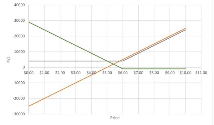
3.1. Synthetic Option Payoff ... 70
4.1. Default Tree for the Cash Market ... 78
4.2. Example of the VaR ... 81
4.3. Corn’s Cash and Futures Prices ... 85
4.4. Soybean’s Cash and Futures Prices ... 86
4.5. Corn’s Best-Fit Copula ... 87
4.6. Soybean’s Best-Fit Copula ... 88
4.7. U.S.-Corn Export Cancellations by China ... 89
4.8. U.S.-Soybean Export Cancellations by China ... 89
5.1. Sensitivity Analysis: Put-Option Strike Price (Corn) ... 97
5.2. Sensitivity Analysis: Default Probability (Corn) ... 99
5.3. Sensitivity Analysis: Probability of Default Before Cash Purchases (Corn) ... 101
5.4. Sensitivity Analysis: Risk-Averse Coefficient (Corn) ... 103
5.5. Sensitivity Analysis: Cash-Price Standard Deviation (Corn) ... 104
5.7. Sensitivity Analysis: Put-Option Strike Price (Soybeans) ... 109
5.8. Sensitivity Analysis: Default Probability (Soybeans)... 111
5.9. Sensitivity Analysis: Probability of Default Before Cash Purchase (Soybeans) ... 112
5.10. Sensitivity Analysis: Risk-Averse Coefficient (Soybeans) ... 113
5.11. Sensitivity Analysis: Cash-Price Standard Deviation (Soybeans) ... 114
CHAPTER 1. INTRODUCTION 1.1. Overview of Study
Many risk factors in any business operation caused instability for the firm’s profitability. The instability creates more difficulty for the firm to operate in today’s highly competitive and risky business environment. Managing risk is one of the most important functions of the business operation. Risk management is particularly important for commodity trading because the
industry is highly competitive and risky, and the firm or trader does not control the price for the commodity that they are trading. The uncontrollable price fluctuation of the traded commodity is called price risk. In order to mitigate the risk, traders hedge the price risk with commodity derivatives that are traded at public exchanges. Also, traders can approach risk management mathematically via the portfolio theory. The main objective of this study is to develop a hedging model by applying the portfolio theory and to determine the optimal hedging decision for traders who are experiencing price and default risks. There are two approaches to analyze the optimal hedging decision. Theoretical analysis and empirical analysis. The theoretical analysis is derived, mathematically, as the optimal hedging decision. Whereas the empirical analysis uses stochastic optimization.
1.2. Problem Statement
Risks for commodity trading are price risk, quantity risk, weather risk, and operational risk as well as counterparty or default risk, and many others. Two types of risks are considered in this study: price and default risk. The price risk refers to fluctuation in the asset’s price. To reduce the price risk, a trader hedges the commodity price with commodity derivatives such as futures or options. The hedging is an act of taking the opposite position in similar and related markets to reduce the price risk. When the underlying position is hedged, the loss from one
market is offset by another market. Default risk is also considered in this study. The default risk describes when the counterparty defaults on the contractual obligation. Default risk is a special type of quantity risk has varying sizes for the quantity that is traded. Recently, the occurrence of defaults is increasing, and traders are more cautious about the default risk in the commodity market.
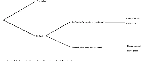
Due to a significant increase in demand for commodities, particularly in China, many traders encountered defaults from Chinese buyers. For example, China has significant purchasing power in the world soybean market because it is the largest buyer of world soybeans. China imported approximately 70.40 million metric tons during the 2013 to 2014 marketing year (Production, Supply, and Distribution). This purchasing power allows Chinese buyers to default on soybean shipments. The soybean defaults occurred during the 2003 to 2004 marketing year and in 2014 (Solot, 2006; and Thukral & Shuping, 2014). Figure 1.1 shows the soybean-default and soybean-crush margins in China’s Dalian region (Thomson Reuter Eikon 2016d). The figure illustrates that a lower soybean-crush margin increases the chance and number of cancellations.
Figure 1.1. Default and Soybean-Crush Margins in Dalian, China.
-400 -300 -200 -100 0 100 200 300 400 500 600 0 100000 200000 300000 400000 500000 600000 700000 800000 6/2/2010 6/2/2011 6/2/2012 6/2/2013 6/2/2014 6/2/2015 6/2/2016
Similarly, corn and distiller dried grain (DDG) are defaulted by many Chinese buyers due to the import ban of MIR162 varieties in late 2013 to 2014(“China Rejects,” 2013; Farm City Elevator, Inc., 2014). Corn and DDG are one of many cases of defaults that occurred with in agricultural products. Many other instances of defaults are seen not only in agricultural products, but also for other commodities. 1
As an illustration to see the default’s effect on the trade’s profit and loss, suppose that a trader sells grain to an overseas buyer and hedges the entire sale with a futures contract. In this case, the trader has a short position in the cash market and a long position for the futures market. Suppose that the price declined, causing the buyer to default on the purchase contract. The default worsens situation because the loss from the futures position is magnified by a decreased return for the cash position. The futures contract has a limited ability to hedge both the price and default risks. Therefore, we introduce a put option to the hedging model in order to, primarily, hedge the default risk.
1.3. Portfolio Model of Hedging
Portfolio theory originates from Markowitz’s (1952) seminal paper. One of the main objectives is to determine the optimal allocation for a risk-averse investor who is considering the portfolio’s expected and variance return. When portfolio theory is applied to hedging for
commodities, its main objective is to find optimal HR for the futures and option to either
1 Although this thesis addressed the buyer’s default risk with international trading, similar problems exist for the seller’s risk in some countries. As an example, the following message was received from a trader who worked with the former Soviet Union (FSU):
We started this year to actively originate and sell third party grain. Since June, we have purchased 650,000 tons for $100 million. In 2017, we want to trade 2 million tons for $300 million.
While we measure and manage the price risk of our open trading position through a VaR calculation, I am concerned about our counterparty risk. For example, we buy grain forward from Ukrainian farmers and sell it forward to international traders. If grain prices spike in the meantime, farmers might default and we sit on losses, which our trading margin cannot cover. We therefore need to implement a system to measure
maximize or minimize the objective function. Researchers can specify several objective functions. This study includes but not limited to minimum variance, mean-variance (E-V), semivarinace, lower partial moments (LPM), mean-Gini coefficient, minimum value-at-risk (VaR), and mean-VaR (E-VaR). In this study, the E-V and E-VaR are used. Each objective function has advantages and disadvantages. For example, variance minimization is utilized to reduce the portfolio’s variance. Similarly, the E-V framework maximizes the risk adjusted expected return function which approximates the trader’s utility. The variance treats upside and downside risk equally. The equal treatment is the biggest disadvantage of using variance to measure risk because a risk averse trader prefers upside over downside risks. In contrast to variance, VaR is a downside risk measure and only considers the downside risk. This study focuses on E-V and E-VaR for the theoretical and empirical approaches respectively.
Traditionally, portfolio-hedging models assume a known cash position and only hedge with a futures contract. However, default risk is special type of quantity risk, and for this reason we have a put option in the study’s objective function. The default risk is incorporated in the model by assuming that default risk has a probability distribution. Including put options offers more flexibility for hedging, and the asymmetric payoff allows the trader to hedge more efficiently hedge default risk. Integrating the default risk and put option with the hedging model’s development is a major improvement compared to the traditional hedging model. 1.4. Theoretical Approach
A theoretical hedging model which incorporates the default risk and includes the futures and put options is specified. Constructing the theoretical model is based on Bullock and Hayes’ (1992) paper. The theoretical model uses the E-V framework. The cash, futures, and default distributions are assumed to be normal. In order to derive the first and second moments of profit,
Bullock and Hayes’ (1992) theorem is applied. This theorem allows us to split the total payoff function at strike price of the put option. This theorem is useful to bypass the problem caused by the put option’s asymmetric payoff. The major result from the theoretical analysis is the
existence of a global optimum solution that maximizes the E-V function. Global optimum is proved by showing that the optimal futures and put option HRs exist and that the Hessian matrix is negative definite. This result is powerful because, at least theoretically, a solution exists. 1.5. Empirical Approach
The empirical analysis uses Monte Carlo simulation and stochastic optimization to estimate the optimal HRs under default risk. This analysis is conducted for soybeans and corn. The price distributions are lognormally distributed, and the default risk is assumed to be a Bernoulli distribution. The E-VaR is utilized as the objective function because using the VaR as a risk measure is appealing. The E-VaR is appealing because it has an expected profit component while, the VaR is a downside risk measure. The base case optimization result is derived to create a standard for analysis. Alternative hedging scenarios and different objective functions are assumed in order to compare the optimization results. Additionally, sensitivity analyses are conducted to see the effect of changing the variable’s value and the correlation assumption to the optimization result.
From this analysis, traditional naïve hedging is a suboptimal hedging strategy, and surprisingly, the alternative objective functions lead to the equivalent optimization result. Another important result comes from using the copula function instead of the Pearson linear-correlation function. Copula leads to more realistic optimization results because the copula preserves correlation structure between random variables.
1.6. Thesis Organization
This thesis is organized as follows. Chapter 2 is the review of the related literature and the background of the problem. The chapter discusses defaults for both agricultural and non-agricultural markets as well as the academic literature for the hedging’s portfolio model and its findings. Chapter 3 explains the theoretical model. The chapter focuses on mathematical
constructions of the different hedging models and developing the theoretical model for analysis. Chapter 4 contains a detailed explanation about the empirical model and the data used for the analysis. In Chapter 5, both the theoretical and empirical Results are presented and discussed. Chapter 6 contains the study’s Conclusions and implications.
CHAPTER 2. LITERATURE REVIEW 2.1. Introduction
Risk management is one of the paramount aspects of running successful agribusinesses. The managers can reduce risk by taking the opposite position for a commodity derivative such as futures or options in related markets to reduce the risk of physical-commodity price changes. The study’s main focus is to derive the optimal HR by considering the existence of one of the
counterparties’ default risk. In commodity marketing, the default risk is a special case of production, or quantity, risk. If the buyer defaults on the agreed sale, the seller gains zero revenue. However, quantity risk can be hedged with commodity derivatives by taking the position based on portfolio-hedging models. The HR is the futures or options position that is taken with respect to the cash position’s size. For example, if the HR is one, the size of the futures or option contract is equal to the cash position’s size. In order to find the optimal HR, the hedger first needs to think about the definition of the risk for moving forward.
2.2. Risk in Agriculture and Commodity Marketing
In this study, the definitions for risk and uncertainty are treated differently to evaluate the default risk’s effect on the HR. A risky event has probabilistic outcome whereas uncertainty is an event that cannot be associated with probability (Chavas, 2004). In other words, a risk has an associated probability distribution, but uncertainty does not have probability distribution. This distinction is important to analyze the default risk’s impact on the optimal HR. Difficulty arises when the default event is uncertain because without knowing the likelihood of a default, building an analytical model is almost impossible. Because risk and uncertainty are defined, we first review the most common forms of risk in agriculture.
The most notable risks in agriculture are related to price and quantity. Price risk originates from fluctuating commodity prices. By definition, the price risk has associated probability distributions; therefore, the price risk can be measured by using the standard
deviation or variance of a commodity’s historical price or return during a specified time period. A higher price risk means greater standard deviations, and lower a price risk means lower standard deviations. Farmers and producers are subject to significant price risks if the cash market in which they participate has a high standard deviation for the price. For farmers,
understanding of the behavior of the cash market where that they participate is a critical element of risk management (Tomek & Peterson, 2001). Farmers hedge the price risk of their cash position by using the commodity futures and options that are traded at centralized exchanges, such as the Chicago Board of Trade (CBOT), or take forward contract to set a delivery price and time. Without considering the basis risk, transaction cost, and storage cost, the farmer can hedge the entire cash position, which implies a HR of one, by selling an equal amount of futures in the futures market. The HR of one removes the return fluctuation that is caused by the physical commodity’s price movement if the basis risk is zero. Any loss incurred from the cash position due to a decreased price is offset by profit from the short futures position and vice versa.
Similar to the price risk, yield risk arises from the quantity’s fluctuation. This risk is felt by a commodity’s farmers or producers and leads to revenue fluctuations. When a farmer hedges the price risk using futures and options to obtain more stable revenue, he/she has difficulty determining the hedging position’s optimal size due to yield risk. They end up either under-hedging or over-under-hedging relative to the actual production at the end of harvest period. If the producer under-hedges or over-hedges compared to the actual harvest, the hedge may not be optimum.
2.3. Forward vs Futures Contracts
There is difference between a forward contract and a futures contract. Both forward and futures contracts are agreements between buyers and sellers. A forward contract is an agreement between two parties for the delivery of product at a specified future date and price which are written in the contract (Kolb & Overdahl, 2007). In contrast, a futures contract is a highly standardized type of forward contract with more specified contract terms (Kolb & Overdahl, 2007). Moreover, the futures contract is subject to the margin mechanism and clearinghouse procedures that do not exist with the forward contract. The futures contract has margin mechanism and counterparty risk is eliminated by clearinghouse.
The biggest difference between a forward and futures contract is that a forward contract is subject to the counterparty’s default while the futures contract is not. The forward contract is subject to default risk because there are no or limited guarantees in the agreement. Default risk exists because the forward contract is done privately without a clearinghouse; at the same time, because the agreement is done privately, the contractual terms and specifications are negotiable. The reason why a futures contract is not subject to default is because the futures trading goes through organized exchanges such as the Chicago Mercantile Exchange(CME), and are required to go through a clearinghouse. The clearinghouse’s job is to assure that every trader who
participates in the futures trading honors the obligation. The clearinghouse matches the position of every buyer to every seller and the position of every seller to every buyer, and every trader in the market only has an obligation to the clearinghouse (Kolb & Overdahl, 2007). In addition to trading through the clearinghouse, traders must deposit money with a broker when they initiating trade in the futures market. This deposit, the margin, is a financial protection which forces the trader to follow the contractual agreement (Kolb & Overdahl, 2007).
2.4. Defaults in Commodity Marketing and Trading
Many risk types exist in the production and marketing of agriculture. They include yield and price risks. Default risk, or counterparty risk, has become more prevalent in agricultural marketing and commodity trading in general; hence, traders and risk managers find it necessary to hedge counterparty’s default risk, i.e., contract non-performance risk. This section is an overview of defaults instances for agricultural and non-agricultural backgrounds.
2.4.1. Definition of Default
The first step in risk management is to clearly define the risk. The default risk is when one of the parties involved with a transaction reneges on the obligation. Jarrow and Turnbull (1995) identify two sources of default risk. The default occurs when payment is less than agreed payment or the writer of the derivative security defaults (Jarrow and Turnbull, 1995). Zhu and Pykhtin (2007) have similar definition that the counterparty credit risk is when the counterparty defaults before the contract matures and does not make all the promised payments.
2.4.2. Types of Counterparty Credit Risk
In this study, two types of counterparty credit risk exist in agriculture. The first type is a strategic default by one of the parties, and the second type is a non-strategic default. The
difference between these two defaults types is simple. A strategic default occurs when defaulting on the purchasing contract is more beneficial than honoring the original contract. Historically, the strategic default occurs when market volatility increases tremendously. Non-strategic default takes place when exogenous, uncontrollable, factors, such as an import or export restriction, cause the counterparty to default on the purchasing and sales contracts. These default types are the dominant ones that occur in the commodity marketing and trading.
2.4.3. Impact of Defaults on Traders
The default’s impact on the commodity traders is large because of a synergizing effect that comes from both the cash and futures positions. As an example, a U.S. based commodity trader sold soybeans to a crusher in China for $10 a bushel. The trader in the United States is short cash, and the trader hedges the short-cash position with a long-futures position. Suppose that the soybean price drops to $5 bushel, and that the buyer defaults on the contract. The trader has to find new buyer for the cash commodity at lower price than the originally agreed-price also losing the profit from the long-futures position ($5 bushel in this example). This simple example illustrates where the loss is synergized rather than offsetting because no return is coming from the cash position.
2.4.4. Chinese Buyers Defaulting on Soybean
The defaults for the grain-procurement agreement have become more prevalent in the agriculture sector, especially for international commodity trading. The most well-known default case for international commodity trading is by China’s soybean buyers. Historically, China is the world’s largest importer of soybeans. According to the Foreign Agricultural Service (FAS) at United States Department of Agriculture (USDA), China imported 70.364 million metric tons during the 2013 to 2014 marketing year, and this is approximately 62 percent of total world soybean export (U.S. Department of Agriculture, Foreign Agricultural Service, 2015c). The amount imported by China is almost six times greater than the second largest soybean importer, European Union, of 12.538 million metric tons in 2013/2014 marketing year (U.S. Department of Agriculture, Foreign Agricultural Service, 2015c). Due to the amount of soybeans that China imports each year, the country has huge buying power and advantages when buying soybeans
from the world market. Figure 2.1 shows Chinese soybeans imports and its percentage compared to total world export.
Figure 2.1. Chinese Soybean Imports and the Percentage of Imports to World Exports.
During the early 2000s, the soybean-crushing margin, the profit margin for crushing soybeans, in China was considerably high, but the margin decreased when the soybean price started rising. The margin turned and stayed negative during 2003 and 2004 (Solot, 2006). In April 2004, many Chinese soybean crushers contracted to purchase soybeans at $10 a bushel; however, during the delivery time in June to August, the price of soybean dropped to $6 a bushel, which leading to a default on the contract (Solot, 2006).
In 2014, some Chinese soybean buyers defaulted on soybean cargo because they failed to obtain a letter of credit, a document which is issued by a bank to guarantee that the seller
receives full payment when the delivery condition is fulfilled. One goal for letter of credit is to reduce credit risks. When a buyer is unable to fulfill the purchase’s payment, the bank steps in and pays the outstanding amount. Because Chinese importers could not obtain letter of credit from banks and had losses with soybean crushing, the Chinese importers defaulted on at least
57% 58% 59% 60% 61% 62% 63% 64% 65% 0 10000 20000 30000 40000 50000 60000 70000 80000 90000 2011/12 2012/13 2013/14 2014/15 Jun 2015/16 Jul 2015/16
500,000 tons, approximately $300 million, of the U.S. and Brazilian soybean cargo; this action was the biggest default that occurred since 2004 (Thukral & Shuping, 2014).
The Chinese soybean buyers’ 2014 default case raises questions about why soybean exporters did not confirm the letters of credit before signing a purchasing agreement. After the 2004 default, soybean exporters stopped shipping soybeans to China without confirming the importer’s letter of credit. This practice slowly started again and lead to the 2014 default case (Thukral & Shuping, 2014). Also, some trading firms relaxed the letter-of-credit requirement and accepted deposits from clients, particularly clients with well-established relationships (Topham & Shuping, 2014). With China’s 2014 soybean default, some soybean cargo changed the destination of ocean shipping after the default incident. The two soybean shipments that were sold by the Japanese trading firm Marubeni Corp. contained Brazilian soybeans that were headed to China: those soybeans were rerouted to the United States (Plume, 2014).
The cancellation was derived from the USDA’s export-sales reporting system, an export sales reporting program which monitors the 39 commodity sales made to foreign country from the United States on a daily and weekly basis. Commodity exporters are required to report the sale of more than 100,000 metric tons of a commodity to a single destination per day or more than 200,000 metric tons of total sales for single commodity to the one destination in a reporting week (U.S. Department of Agriculture, Foreign Agricultural Service, 2015a). These data are a proxy to illustrate the amount of cumulative sales cancellations for a single commodity that occurred during a particular week. Figure 2.2 represents the cancellation of U.S. soybean sales that were destined for China from 1990 to 2016.
Figure 2.1. Cancellation of U.S. Soybean Sales to China in Metric Tons.
Since 2005, there was an upward trend for China’s cancellation of U.S. soybean sales: the peak was in 2012. From 2013 to 2015, the cancellation level stayed above 2 million metric tons. Although soybean exporters may incur losses from Chinese soybean importers’ defaults, the Chinese soybean market is the most lucrative one in the world due to the country’s quantity of soybean imports. Because of the quantity of China’s imports, Chinese soybean buyers have strong negotiating power over the commodity-trading firms that sell to China. Therefore, credit risk management is becoming more important in the world of commodity trading. According to personal communication with W. W. Wilson Chinese buyers purchased the U.S. soybeans exported from New Orleans, Louisiana region around $1.10 to $1.35 basis price. The soybeans basis price dropped to $0.28 due to cheap ocean freight rate and the competition from Brazil, the Chinese buyers may default on the original soybean contract (personal communication,
November 23, 2016). 28197 18205 382230 619997 350708 1695845 122362 350071 895937 1295807 2042720 1833336 2722926 3029120 2157842 23736282314140 218084 1999 2000 2001 2002 2003 2004 2005 2006 2007 2008 2009 2010 2011 2012 2013 2014 2015 2016
2.4.5. MIR162 Corns, DDG, and Sorghum Exports to China
The United States produced approximately 351 million metric tons of corn, 36% of the world’s corn production, during 2013 to 2014 crop year (U.S. Department of Agriculture, Foreign Agricultural Service, 2015c). In terms of the corn trade, China is not as large of an importer as with soybeans. China imported 3.277 million metric tons of corn in the 2013/2014 crop year (U.S. Department of Agriculture, Foreign Agricultural Service, 2015b). Although China does not import as much corn as it does soybeans, China significantly influences the world’s corn market. Figure 2.3 shows U.S. corn exports to China.
Figure 2.3. U.S. Corn Exports to China in Metric Tons.
A major default case for the corn market is an import rejection of U.S. corn by the Chinese government due to an unapproved genetically modified (GM) trait that was found in imported corn. This specific, unapproved GM corn found was SYN-IR162-4, the so-called MIR162 trait, developed by Syngenta Seeds, Inc. The MIR162 corn for approved in major corn markets, except China, and the first rejection of the U.S. corn occurred on November 18, 2013
0 100000 200000 300000 400000 500000 600000 700000 800000 900000 2012-2012 2013-2013 2014-2014 2015-2015
(Farm City Elevator, Inc., 2014). According to the weekly report published by Informa
Economics (2014), the purpose of restricting GM corn is to increase the consumption of China’s domestic corn. The landed value of the U.S. corn in China is significantly cheaper than China’s domestic-government-supported corn price which incentivizes consumers to purchase other overseas grains for feedstuffs. Figure 2.4 shows the cancelation of the U.S. corn sales to China from 1999 to 2016 in metric tons. In 2014, there was a huge spike in the cancellation of U.S. corn, primarily because of the MIR162 trait’s rejection by the Chinese government.
Figure 2.4. Cancellation of U.S. Corn Sales to China in Metric Tons.
In addition to the U.S. corn exports that were affected by the China’s import rejection due to the unapproved MIR162 varieties, the byproduct of corn crushing, which is called distillers’ dried grain (DDG), and sorghum exports to China also affected by rejections. DDG is a
byproduct of ethanol which is produced with a process called crushing. The physical crushing is the process of converting corn into ethanol and DDG. Usually, DDG is used for a livestock feed
1 0 0 885000 0 0 25540 8106 0 0 0 242456 899 643899 819129 2767627 99350 0 1999 2000 2001 2002 2003 2004 2005 2006 2007 2008 2009 2010 2011 2012 2013 2014 2015 2016
because it is a rich, high-protein source. On December 27, 2013, Xinhua reported that two batches, approximately 758 tons, of the U.S. DDG with soluble were rejected because Chinese officials found them to contain the MIR162 strain (“China Rejects”, 2013). Because MIR162 corn varieties are unapproved GM varieties, China imposed inspection of DDGs imports in July 2014, and any shipment with DDG purchases after August 18th is required to have MIR162 free
certificate (Informa Econmics, 2014). Chinese authorities’ inspection apparently caused a decrease in the U.S. DDG exports to China as which is shown in the Figure 2.5 (United States Department of Agriculture, Foreign Agricultural Service, 2015b).
Figure 2.5. U.S. DDG Exports to China.
After the import ban for U.S. corn and the DDG inspection, U.S. sorghum exports to China increased more than 15-fold in 2014, and some Kansas grain elevators offer a 10% premium for sorghum above the corn price because sorghum does not have a futures market and because corn is used as reference for sorghum prices (Kesmodel, 2015). This phenomenon indicated that sorghum is a substitute for China’s corn-import demand. Chinese importers moved
0 100000 200000 300000 400000 500000 600000 700000 800000 900000 1000000 2012-2012 2013-2013 2014-2014 2015-2015
their interest to purchase U.S. sorghum as an alternative, cheaper feedstuff, and the U.S.-corn import restrictions likely had a positive impact on U.S. sorghum exports to China (Informa Economics). The Figure 2.6 shows the increase in U.S. sorghum imported by China (United States Department of Agriculture, Foreign Agricultural Service, 2015c).
Figure 2.6. U.S. Sorghum Imports by China in Metric Ton.
Because the imported U.S. corn contained unapproved MIR162, there were many interesting consequences for corn, DDG, and sorghum. MIR162 corn was approved by Chinese officials during at the end of 2014. On December 22, 2014, Syngenta announced that MIR162 received formal import approval from China’s regulatory authorities (Syngenta AG, 2014).
2.4.6. Defaults for the Wheat Market
Another major loss in the grain market is caused when one of the largest wheat-exporting countries, such as the Russian Federation, bans grain exports and establishes quotas. This
decision has effects on wheat importers because they may have to find a new seller with a higher price. According to the U.S. Wheat Associates (2011), governments’ export bans cause
contractual prohibition and cancellation, creating a higher price than originally agreed upon for importers. Russia is known for banning grain exports, particularly in 2010, to deal with poor
0 2000 4000 6000 8000 10000 12000 2011/12 2012/13 2013/14 2014/15 2015/16Jun 2015/16Jul
production due to drought and rising food prices. Additionally, Russia changed the tariff rates for wheat that was exported overseas (Blas, 2010; Global Agricultural Information Network, 2014; Kolesnikova, 2010; Kramer 2010; Vassilieva & Pyrtel, 2007). Because Russia is one of the largest wheat producers, a buyer is forced to find a different wheat seller. In 2010, Many Russian wheat buyers had to find an alternative seller with price that was $100 per metric ton above the original purchase price (U.S. Wheat Associates, 2011). According to the U.S. Wheat Associates (2015) Russia’s state intervention creates extreme price volatility which is shown in Figure 2.7. The figure shows the effect of five Russian interventions from 2007 to 2014, on the Kansas wheat-futures price. The increases were as follows: 30% in two 2014 interventions, 45% with the 2012 intervention, and 100% for the 2007 and 2008 interventions (U.S. Wheat Associates, 2015).
Figure 2.7. Russia’s Wheat-Export Intervention and Kansas Wheat Futures Prices.
An extreme price move causes a supplier to default on the agreed selling contract. In 2012, the rise in the global commodity prices, triggered by a drought in the United States
incentivized grain suppliers to default on the delivery contract because that contract created a loss from rising commodity prices (Hogan & Saul, 2012). With international grain trading, there is a function to force an agreement between counterparties. Most international grain contracts requires as 10% performance bond which the seller has to pay to buyer when a contract default occurs (Hogan & Saul, 2012). With a 10% performance bond, the seller defaults when better than keeping original agreement (Hogan & Saul, 2012). Defaulting on the sales contract may have a negative influence on the long-term relationship, but with extreme price movements defaulting on the sales agreement may be more beneficial for suppliers.
2.4.7. Defaults for the Cotton Market
An incidence of supplier default happened with cotton trading due to an unexpected price rise in the global cotton market. According to Pirrong (2014) and Kub (2012), the cotton
market’s contract performance risk emerged in during late 2010 to 2011. At that time, the world cotton price tripled, which led sellers to default on physical purchasing contracts; also when prices came back down, consumers defaulted on the contracts (Kub, 2012; Pirrong, 2014). With this unexpected rise in the cotton price, Glencore suffered when suppliers defaulted on
purchasing contracts and had to purchasing cotton at a higher price (Kub, 2012). 2.4.8. Non-Agriculture Default Cases
A similar default case happened with the iron-ore and coal trade in China. According to Wong and Fabi (2012), there were at least six coal-cargo defaults as well as defaulting iron-ore contracts because of the price drop. Wong and Fabi (2012) said that the default was sparked by the drop in global, thermal coal benchmark prices to two-year lows and the increased
iron-ore trader in Wong and Fabi’s (2012) article was a typical example of a buyer defaulting on a contract when the price is fell:
We ourselves have had one of our buyers default on us after just a few hours. We sold the cargo to an end-user in China and a few hours later the buyer came back, saying “the market’s falling too fast we want a lower price’.” (p. 2)
We analyzed the default cases in both the agricultural and non-agricultural markets, and cancellation and default were not uncommon events. In the next section, an overview of the portfolio model of hedging is discussed.
2.5. Portfolio Hedging Models
The conceptual framework used to determine the optimal HR builds on portfolio optimization or the so-called modern portfolio theory, which was first published in Markowitz (1952). This model focused on the fact that investment’s future return is dependent on the selection of the portfolio by considering the expected return and the variance of return as portfolio’s desirable and undesirable aspects, respectively. With an analytical model that has finite number of securities, Markowitz (1952) formulated an investment rule called the expected return – variance of return (E-V) rule. This rule states that an investor chooses an efficient portfolio from a set of possible combinations for the portfolio’s expected return and variance. This rule implies that an investor can select a portfolio by considering its E-Vs. Therefore, the investor can select a portfolio with the minimum variance of return or can accept more return variance to obtain a higher expected return. E-V is the portfolio’s risk-return tradeoff. Hedging the cash position with futures and options by determining the optimal HR is the portfolio optimization, and there are different approaches to use when setting the objective function.
In order to calculate the optimal HR, both the theoretical framework and estimation procedures of the optimal HRs are important. Many of the HR’s theoretical models are different and based on the objective function’s maximization or minimization. The portfolio hedging models can be classified as minimum variance, utility maximization, and risk-adjusted return functions. With the minimum-variance hedging model, the hedger selects a HR that minimizes return’s variance. Under the utility-maximization framework, the objective is to maximize the utility. The adjusted return is similar to the expected utility maximization; however, risk-adjusted return is not associated with any specific utility functions.
2.5.1. Minimum-Variance Hedging Model
The minimum-variance hedging model does not reflect the return which the hedger seeks from the selected portfolio. With the portfolio theory of hedging, the position in the cash market is fixed, and the hedger has required to decide how much of the fixed cash position should be hedged (Ederington, 1979). Johnson (1960) developed a minimum-variance hedging model and theoretically analyzed how the hedger takes a position in the futures market to reduce the portfolio’s variance of return which is caused by the commodity’s price risk. Similarly,
Ederington (1979) developed the minimum variance hedging model and conducted an empirical analysis assuming cash position in the Government National Mortgage Association’s (GNMA) 8% Pass-Through Certificates, Treasury-Bill (T-Bill), wheat, and corn, and these were hedged with corresponding futures contracts. Both Johnson (1960) and Ederington (1979) derived the optimal HR from the variance of return equation, which is the ratio of the covariance of the spot and futures market, and the variance of the futures market. The derived, optimal HR equation was extended to formulate a measure of hedge effectiveness. The hedge’s effectiveness is measured by the square of the correlation the spot and futures market. If the correlation for the
commodity’s price movement in the spot and futures market is one, the loss from one market is exactly offset by the profit made from the other market (Johnson, 1960). With this measure of hedge effectiveness, the lower the correlation for the price movement in the spot and futures market is an indication of a bad hedge because the loss from the spot market due to adverse price movement may not be offset by the profit made with the futures market. Ederington (1979) found that GNMA futures market was a more effective hedging instrument than the T-Bill market for risk-avoidance purposes.
2.5.2. Mean-Variance Hedging Model
Instead of only focusing on minimizing the portfolio’s variance, the E-V model focuses on both the portfolio’s expected return and variance to determine the optimal HR. One may consider that the variance HR is just a special case of the E-V HR. The minimum-variance HR is consistent with the E-V framework when the hedger is infinitely risk averse or when the expected futures’ price change is zero. When the expected future price change is zero, it is pure martingale process (Chen, Lee, & Shrestha, 2003). Many studies incorporate the E-V approach to find the optimal HR (Blank, Carter, & Schmeising, 1991; Cecchetti, Cumby, & Figlewski, 1988; Howard & D’Antonio, 1984; Hsin, Kuo, and Lee, 1994). These studies are utility maximization under the E-V framework which aims to enhance the minimum-variance hedging model. With the E-V framework, the utility function, which the hedger is willing to maximize, is defined in terms of the expected return and variance for the hedged portfolio. Because only the first two moments of distributions are involved with the V utility function, E-V framework can be easily applied for risk analysis (Chavas, 2004).
The theoretical, optimal HR was derived in Blank et al. (1991): it maximized the expected utility of the hedger and included the expected return and variance for the hedged
portfolio as well as the hedger’s risk-aversion parameter. From this optimal HR formula, Blank et al. (1991) concluded that the formula had two sources of demand for the futures: hedging demand and speculative demand. The hedging demand for the utility-maximizing HR was the same as the minimum-variance HR, and the speculative demand showed hedger’s expectation for the hedge’s return because for speculative demand formula includes hedger’s risk parameter (Blank et al., 1991). Blank et al.’s (1991) approach was the utility-maximization approach under the E-V framework where the hedger tried to maximize the utility based on the mean, variance, and risk aversion parameter.
Because many researchers illustrated the unrealistic nature of minimum variance hedging, Cecchetti et al. (1988) argued that the minimum-variance hedge was not optimal because it did not consider the expected return and the time-varying distribution of the spot and futures prices. Cecchetti et al. (1988) assumed that the hedger had log utility and tried to
maximize the expected-utility function with the time-varying joint distribution of spot and futures returns which is estimated using the autoregressive conditional heteroskedasticity (ARCH) model. Cecchetti et al. (1988) also argued that the hedge effectiveness should be measured in terms of the expected utility or the return from the certainty-equivalent. Using the empirical result based on hedging the 20-year Treasury bond in the post-sample and in-sample periods, Cecchetti et al. (1988) found that log-utility maximization is better than the minimum-variance hedge when they compared the returns’ certainty-equivalent.
Hsin et al’s (1994) model hedges the currency exchange-rate risk with the currency’s futures and options. Under the assumptions of the negative-exponential utility function, hedger’s constant absolute risk aversion (CARA) and the normal return distribution, the expected utility maximization depends on the utility function with portfolio’s mean and variance (Hsin et al,
1994). Additionally, Hsin et al. (1994) measured the hedge effectiveness as the difference
between the certainty-equivalent of the hedged and spot position. Hsin et al. (1994) conducted an empirical study and concluded that the currency futures are a better hedging tool than the
currency options regardless of whether the options are synthetic futures or delta/gamma hedges. Under the E-V framework, Howard and D’Antonio’s (1984) approach includes the risk-free return in the expected utility function. This approach is rather unique approach compared to other approaches. The hedger can hold a risk-free asset in the hedged portfolio to reduce the portfolio’s risk. The purpose of holding futures position is not solely on the reduce portfolio risk, but it also aims to improve the risk-return characteristic (Howard & D’Antonio, 1984).
Therefore, the hedger maximizes the utility function which depends on the differences for the expected return from the spot and futures positions, the return from the risk-free asset, and the portfolio’s standard deviation for spot and futures positions (Howard & D’Antonio, 1984). The major finding from Howard and D’Antonio’s (1984) is risk-return relative. The risk-return relative shows spot and future relative return attractiveness. The relationship between risk-return relative and the correlation for spot and futures prices show is important. This relationship
defines the hedger’s activity taking a futures position. If the risk-return relative is greater than the correlation, the hedger long futures contract. If risk-return relative is smaller than correlation coefficient, the hedger shorts futures contract. If risk return-relative is equal to the correlation coefficient, the hedger does not hold any futures position (Howard & D’Antonio, 1984).
The expected utility-maximization approach starts with an assumption for the utility function. Lence (1995, 1996) investigated the value of better approximation for the minimum-variance hedge by maximizing the expected utility of the risk-averse hedger’s terminal wealth. One of Lence (1995, 1996) contributions was relaxing the assumptions that are ignored by most
hedging literature: including the transaction cost and margin requirement. Additionally, Lence (1995, 1996) assumed that the hedger can borrow and lend capital and can also invest his/her own capital into an investment, yielding a certain return. Both Lence (1995, 1996) measured hedge effectiveness in terms of the hedger’s opportunity cost to select a suboptimal return instead of the optimal return. Lence (1995) assumed that the distributions for the return from spot, futures, and alternative investment were joint normal distributions and that the utility function was CARA. Lence (1995) conducted a simulation of the hedger’s behavior, considering the estimation risk, and found that value of better estimation for the minimum-variance hedge is insignificant and that the minimum variance hedge with a relaxed assumption resulted in the optimal hedge being significantly different than the usual assumptions. Lence (1996) relaxed the assumptions made in Lence (1995), one by one, to see the effect of changing the minimum-variance hedge’s value. The biggest assumption changes made from Lence (1995) to Lence (1996) were stochastic production and not allowing all initial wealth to be invested into production. From the simulation results, Lence (1996) concluded that, with increased risk-averseness, the stochastic production reduced the optimal HR and the opportunity cost of not hedging at all to futures. The alternative investment opportunity induced the optimal HR to be proportional to the correlation between the alternative investment and futures prices.
2.5.3. Mean-Value-at-Risk Framework
E-VaR is a framework that adjusts the expected return with portfolio’s VaR. The objective function is classified as risk-adjusted return function. This framework is gaining popularity for portfolio selection and hedging. This framework is used for the empirical analysis in Chapter 4. One of the early studies using E-VaR was conducted by Alexander and Baptista (2002). They compared the E-VaR portfolio selection to E-V, assuming a multivariate normal
distribution of assets. Alexander and Baptista (2002) concluded that, as the VaR confidence interval increases, the minimum VaR converges to the minimum variance while the E-VaR converges to E-V. Alexander and Baptista (2002) also proved that E-VaR approximately maximizes the expected utility of a risk-averse agent.
When hedging, Awudu, Wilson, and Dahl (2016) used the E-VaR framework to hedge input and output price risks for ethanol. Using a stochastic optimization, they determined the E-VaR maximizing HR for three different hedging strategies: short corn, long corn, and hedging the crush margin. With the short-corn strategy, the producer sold all outputs and was left to buy corn. The long-corn strategy assumes that corn was purchased and that the output was sold as futures. The third strategy was to hedge the crush margin. With this strategy, the producer did not sell output and, instead, purchased inputs. The optimization result concluded that short corn was the best strategy because it had the highest E-VaR value.
2.5.4. Other Hedging Frameworks
For the E-V analysis to be consistent with the expected utility-maximization principle, restrictions need to be imposed on the utility’s function and return distribution. Chen et al. (2003) stated that the utility function had to be a quadratic function and that the return’s distribution to be a normal distribution. If these assumptions were not made, then the HR may not be optimal with respect to the expected utility-maximization framework (Chen et al., 2003).
All types of hedging paradigms, the minimum-variance hedge, E-V, expected utility maximization, and risk-adjusted return have strengths and weaknesses. Minimum variance only focuses on the hedged portfolio’s variance. E-V approach has a restriction for the utility function and the return’s distribution to be consistent with the expected utility maximization. The E-V framework is negative utility function. Therefore, one of the most important specifications is the
utility function and for the portfolio’s return distribution. Considering the restrictive assumptions about the hedging models mentioned so far, there is high demand to develop a hedging model which has less-restrictive assumptions about the hedger’s utility function and return distribution.
Hedging models which lessens assumptions about specific utility functions and the return’s distribution utilizes the semivariance, lower partial moment (LPM), Gini coefficient, minimum value-at-risk (VaR), and E-VaR. The purpose of applying semivariance in the hedging model is to hedge against the downside risk instead of portfolio’s entire risk. With the E-V framework, the return’s variance is used to quantify the portfolio’s risk; however, variance treats both upside and downside risks equivalently. Therefore, under the E-V framework, the hedger has to sacrifice possible gain. Realistically, the hedger and investor favor upside risk and dislike portfolio’s downside risk. A theoretical treatment of risk management’s semivariance is done by Hogan and Warren (1974). Turvey and Nayak (2003) formulate a semivariance-minimizing hedging model for agricultural commodities to hedge the downside risk, and this model is free of prior assumptions about the distribution’s shape. Utilizing the numerical approach instead of the econometric approach to calculate the HR, Turvey and Nayak (2003) conclude that a minimum semivariance hedge protects the hedger from downside risk more than the minimum variance hedging model. In general, the magnitude of the protection obtained with semivariance over the minimum variance is uncertain because the semivariance hedge is highly responsive to the distribution of the cash and forward positions as well as the hedger’s target return.
The LPM hedging model’s focus is same as the semivariance model. The LPM focuses on the portfolio’s downside risk. Bawa and Lindenberg (1977) developed the theoretical framework of LPM, and it does not assume return’s distribution. The LPM framework is a
the LPM framework (Bawa & Lindenberg, 1977; Eftekhari, 1998). Eftekhari (1998) formulated a hedging model which minimizes the LPM and numerically computed the LPM-minimizing HR and the minimum-variance HR to hedge the Financial Times Stock Exchange 100 (FTSE-100) index’s return with FTSE-100 index futures. Eftekhari (1998) concluded that the hedger should use minimum variance if he/she is interested in hedging the return’s volatility and use the LPM to hedge the downside risk.
Yitzhaki (1982, 1983), Lerman and Yitzhaki (1984), and Shalit and Yitzhaki (1984) proposed an approach to use Gini’s mean difference, which measures income inequality, as a measure of variability in the field of finance. The mean-Gini framework makes no assumptions regarding the hedger’s utility function and return distribution. This framework is consistent with first-degree and second-degree stochastic dominance (Cheung, Kwan, & Yip, 1990). Cheung et al. (1990) compared the efficient frontiers of E-V and the mean-Gini framework by using five foreign currencies’ futures and options. Cheung et al. (1990) concluded that currency futures are a better hedging instrument than currency options with the minimum-variance and minimum mean-Gini hedging approaches. The E-V framework futures were a better hedging instrument; however, the mean-Gini approached had better options as a hedging instrument. Although the frameworks obtained different conclusions for the hedging instrument, it is difficult to ignore the loosened assumption for the utility function and return distribution.
In order to solve the problems with minimum variance, E-V, and the expected utility-maximization frameworks, researchers created semivariance, LPM, mean-Gini coefficient, and E-VaR hedging models. Each newly framed models had different assumptions and
specifications, and these models had a big advantage: not relying on the return’s distribution. The portfolio hedging model has the goal of either minimizing risk or maximizing the utility function
depending on the model specifications. One of the most important assumptions to make when formulating a hedging model is the hedger’s utility function and return distribution. The different assumptions and specifications for the utility function and return’s distribution of the hedging models may lead to totally different optimal HRs. Comparing the hedging models can be done by using hedge effectiveness or the certainty equivalent of returns for each model. Based on the current research done about the portfolio model of hedging, there is no best model to hedge the risk due to the different assumptions made.
2.5.5. Hedging with Options
Instead of hedging a commodity’s price risk with a futures contract, option contracts are a useful hedging instrument for the industry. Bullock, Wilson, and Dahl (2003) analyzed a bread baker’s hedging demand for futures and options with the E-V framework. Bullock et al. (2003) derived three conclusions regarding the use of options as a hedging instrument. The demand for options as a hedging tool is always zero; options are a less-effective hedging instrument than futures because the delta is lower than one while the futures’ hedging demand is not affected, including options that are available as the portfolio’s hedging instrument (Bullock et al., 2003). Finally, the existence of bias in the futures or options markets as well as the difference between the firm’s expected and actual price, allows non-zero speculative demand for options to be an optimal solution (Bullock et al., 2003).
Bullock and Hayes (1992) applied the E-V framework and used the futures and put options as the hedging instrument. Utilizing the statistical theorem, the investor only needs to focus on the price distributions’ mean and variance. The study found that futures are a primary hedging instrument for the cash position and are used for speculation when the price
price distribution’s variance changes. The study also proved the existence of undiversifiable risk because the relationship between the period-two futures price and put option price is not one-to-one relationship because there are many futures prices for a worthless options price. Due to the undiversifiable risk, the delta neutral hedge needs adjustment. All these results are consistent with and without including the basis risk in the payoff function.
2.6. Previous Literature About Default Risk
In the field of the counterparty credit risk, most of the previous literature focuses on three main areas: the systematic risk of default risk in derivative contracts and regulating the over-the-counter (OTC) market, the evaluation of derivative contracts that are subject to over-the-counterparty risk, and the risk-management strategy with default risk (Korn, 2008). The focus of this study is to find the optimal HR by considering the price and default risk, so the problem is categorized as a risk-management strategy with default risk. Forward and futures contracts are similar; however, a forward contract is subject to counterparty risk, whereas a futures contract is not subject to counterparty risk.
The problem of hedging the counterparty’s default risk is similar to hedging quantity risk. The problem is similar because the forward contract’s seller loses a portion or the entire revenue that was supposed to come from the sale using the forward contract. This study’s main goal is to find a solution for the portfolio model of hedging by considering price and default risk.
2.6.1. Risk Management with Counterparty Default Risk
Previous literature about the default risk’s effect on a firm’s risk-management strategy is most closely related to this study’s problem. Mahul and Cummins (2008) used the expected utility-framework to analyze the firm’s hedging and production decision when the company uses vulnerable, which is subject to counterparty default, forward and options contracts as hedging
instruments. Mahul and Cummins (2008) assumed that the counterparty’s default risk is endogenous: the counterparty’s default depends on the hedging firm’s decision. Mahul and Cummins (2008) showed, mathematically, that, when vulnerable and subject to counterparty credit risk, a forward contract is the only hedging instrument. The vulnerable forward contract encourages the hedging firm’s production to be lower than the non-vulnerable forward contract. Mahul and Cummins (2008) also showed that, under certain conditions, the optimal forward contract is less than the firm’s production. When the vulnerable-option contract, a long-put option, can be used as hedging instrument, the optimal HR contract is one (Mahul & Cummins, 2008).
Similar to Mahul and Cummins (2008), Korn (2008) used the expected
utility-maximization framework to solve for the optimal hedging and production decisions of a risk-averse, competitive firm under the price uncertainty with an exogenous default risk. The firm’s hedging decision does not affect the counterparty’s default. Korn (2008) found that, if the
expected profit for a forward contract is zero, the HR is independent of default risk: that is, a HR of one is the optimal. This result also implies that the HR is the same with and without default risk if the forward contract’s expected profit from is zero. Korn (2008) extended the basic model to include a stochastic recovery rate. The stochastic recovery rate implies only some partition of gain from forward contract is lost due to default. With the stochastic recovery rate, Korn (2008) obtained a counterintuitive result, a HR above one with a stochastic recovery rate and an
exogenous default risk. This conclusion was different from Mahul and Cummins’ (2008) endogenous default risk. The possible explanation was that the endogenous default-risk assumption was affected by absolute size of a hedging company’s forward contract which induces under-hedging: additionally, the hedge’s speculative and default components have an
effect on the forward position’s absolute size (Korn, 2008). Furthermore, Korn (2008) suggested using default-risky credit derivative if forward contract is subject to default risk to diversity default risk between the forward contract and credit derivative.
Another approach taken by industry professionals to measure credit exposure is credit valuation adjustment (CVA) which is primarily used for OTC derivative contracts. The CVA allows banks to measure market value of credit exposure of derivative contract, and it is defined as difference between the risk-free portfolio value and true portfolio value subject to the default risk (Zhu and Pykhtin 2007). According to Zhu and Pykhtin (2007), there are three main
components for calculating the distribution of a counterparty’s credit exposures: scenario generation, instrument valuation, and portfolio aggregation. The first step to calculate the credit exposure is to generate a scenario for a future market with a by computer simulation by using evolution models of a risk factor for a fixed set of dates. The instrument is valued using the scenario created for each simulation date and risk factor in the first step. Portfolio aggregation is the sum of all contract-level counterparty credit exposure when considering the netting
agreement for each simulation date and risk factor. Modeling the credit exposure and calculating the CVA allows a firm to quantify and hedge its counterparty credit exposure.
In this study, the put option is used as the hedging instrument. Mahul and Cummins (2008) introduce the vulnerable option, subject to counterparty risk, into the hedging. The option allows traders and risk managers to flexibly manage risk when the only incurred loss is the option premium. The Theoretical Hedging Model with a put option is described in the Chapter 3. 2.7. Summary
The purpose of this chapter is to review previous studies about risk management. Several risks exist in agribusiness, primarily a commodity’s price and quantity. These risks induce
variability into the profit that is measured by the profit’s standard deviation. These risks are conventionally hedged with commodity futures and option contracts; however, hedging the default risk, a special case of quantity risk, is difficult for both industry professionals and academic researchers. In recent years, the size and frequency of cancellations in the agricultural market have increased. At the international level, the cancellation of soybean and corn sales grown. There are many factors and reasons for this default. Regardless of the reason for the defaults, risk managers and traders need to increasingly manage that default risk.
In order to hedge a risks, researchers developed portfolio hedging models based on Markowitz’s (1952) seminal paper. Each one has different specification of the objective function that is subject of optimization. The minimum variance’s objective is to minimize the portfolio’s variance whereas the E-V maximizes the utility function that considers the portfolio’s return and variance. The E-V framework requires the quadratic utility function and a normal return
distribution to be consistent with the expected utility-maximization. Similarly, the E-VaR is discussed as an example of risk-adjusted return function. Managing the default risk is studied in few papers, such as Korn (2008) and Mahul and Cummins (2008). Both Korn (2008) and Mahul and Cummins (2008) analyzed the theoretical hedging decision of a risk-averse firm with default risk. Additionally, CVA is the latest methodology utilized to evaluate the counterparty’s credit risk.
CHAPTER 3. THEORETICAL HEDGING MODEL 3.1. Introduction
Several portfolio hedging models were reviewed in the Chapter 2. Those models are classified into three approaches: minimum variance, expected utility-maximization and risk-adjusted return. The results from these models can be used by hedgers for decision making. This chapter extends portfolio hedging model to include the counterparty’s default risk; the model uses the option contract as the hedging instrument. The default risk is a special case of quantity risk which the firm faces when counterparty defaults on the originally agreed sales for each transaction. This chapter is organized in five sections: first, the basic portfolio model for hedging the price risk is explained in detail; second, the models to hedge both price and quantity risk with a futures contract are developed; third, the basic models are extended to include options; fourth, two default risk models are discussed. Last, the mathematical analysis of the default risk model that hedges the price and default risks with futures and options is conducted.
3.2. Portfolio Model of Hedging the Price Risk
The portfolio model of hedging is a common agricultural problem: the model analyzes the hedging price risk with forward, futures, and/or options contracts. One of the main
assumptions made in the models for hedging the price risk is that the hedger has a fixed and known amount of inventory and is only interested in hedging the price of that inventory.
Traditionally, portfolio models are developed using the one of minimum variance, E-V, or utility maximization frameworks. Based on a seminal paper by Markowitz (1952), Johnson (1960) and Ederington (1979) applied the minimum variance to hedging commodity price risk and the GNMA 8% Pass-Through Certificates, respectively. Blank et al.’s (1991) developed a hedging