Does Fair Value Accounting Reduce Prices and Create Illiquidity?

Does Fair Value Accounting Reduce Prices and Create

Illiquidity?

Abstract

Concerns about the use of fair value accounting commonly focus on the sensitivity of market prices to exogenous liquidity shocks. In this paper, we show that the use of fair value accounting for assets without an active market endogenously creates illiq-uidity. The underlying mechanism is the discretion in fair value reports when prices are unavailable. Firms use this discretion to report aggressively, leading to two market eects. On the plus side, by revealing an upper bound on an asset's value, fair value reporting leads to lower prices than would occur in a conservative regime. This is an indication that prices are more ecient than under conservatism, as the reports protect investors from paying information rents. The downside is that fair value reports cannot credibly convey a lower bound on an asset's value, causing illiquidity. We conrm these eects in a laboratory experiment.

Keywords: Financial crisis, fair value accounting, incomplete preferences, ambiguity, experiments, auctions

1 Introduction

Much of the controversy over fair value accounting is related to the eects of using fair value for an illiquid asset. The supply side of the market is understood. An exogenous price drop may trigger selling pressure due to regulatory requirements, or due to concerns over the externality that other agents' trades generate. Allen and Carletti (2008) and Plantin et al. (2008) address these eects of fair value on asset supply, and we do not revisit the questions they raise. By contrast, we are unaware of any work systematically addressing the eects of fair value on the demand side of the market. Our purpose in this paper is to ll this gap.

Unlike fair-value driven supply shocks, the eects of fair value on asset demand do not come from exogenous changes to prices or liquidity. Instead, the eects of fair value on demand are concentrated in assets for which there is no active market price, in which rms use models to estimate fair values. The absence of a well-dened, veriable market price creates discretion in a rm's reported fair value of an asset, as the auditing literature has documented (see Schmidt (2009) and Bratten et al. (2013, 10)). Firms use their discretion to report aggressively, as is commonly found in laboratory experiments (King and Wallin, 1991, Forsythe et al., 1999) and in empirical research (Beatty and Weber, 2006, Dechow et al., 2010, Blacconiere et al., 2011). Investors respond by discounting reports for model-based fair values, as Goh et al. (2009) observe; for a discussion, see Laux and Leuz (2010).

This practice of discounting model-based fair value reports has two main eects. First, although the demand eects of fair value lead to lower asset prices than under a conser-vative reporting regime, the prices are more informationally ecient. The reason is that the aggressive equilibrium reports reveal upper bounds on an asset's value to the market, protecting investors against paying information rents. That is, although model-based fair value reports are upwardly biased, they provide information that investors value (Song et al., 2010, Magnan et al., 2015). By contrast, a conservative reporting regime provides investors with a lower bound on an asset's value, eectively imposing a sanitized report as in Shin

(1994). This leaves investors vulnerable to paying information rents.

Second, using fair value for assets without an active market (known under Statement of Financial Reporting Standards 157 as Level 2 or Level 3 reports, which we refer to as mark-to-model reports) causes endogenous drops in liquidity, in comparison to a conservative regime. That is, prices under fair value use information more eciently than those under conservatism, provided that trade occurs. But this gain in price eciency comes with a decrease in liquidity, which may reduce overall market eciency. The reason for the loss of liquidity under fair value is symmetric to the reason for the disappearance of information rents. In equilibrium, rms can report only aggressive fair value estimates, leaving investors in the dark about credible lower bounds on asset values. A conservative regime necessarily provides a lower bound, giving rms a credible way to prevent investors form becoming overly pessimistic.

After developing the theory behind the above argument, we use a laboratory experiment to demonstrate the eects of using mark-to-model reporting on demand. As predicted, sellers take advantage of their discretion, issuing highly aggressive reports that clearly rst-order stochastically dominate their secret reserve prices.

We then turn to the market's reaction to aggressive reporting, which generates the de-mand eect noted above. Using a matched pairs design, we compare trading behavior in conservative and aggressive reporting regimes. As expected, we nd that both the bid dis-tribution and the highest bid are lower under aggressive reporting than under conservative reporting. Prices fall due to a disappearance of information rents. We do not observe supply eects on prices, as seller reserve prices are indistinguishable across treatments.

We also nd that fair value leads to illiquidity, compared with conservatism. Participants facing aggressive reports traded in just under half of the rounds. Their counterparts in the conservative treatment traded in nearly 3/4 of the rounds.

in markets with ambiguous fair values, some remarks about the nancial crisis are in order. Our theory predicts and our experiments replicate the pattern seen in the crisis, but the driving force is not the bursting of a bubble or the arrival of a panic, i.e. a negative bubble. In fact, we obtain our predictions in a one-shot setting. To the extent that the forces we identify were in place in the crisis, the implication is that the friction was illiquidity, not the drop in asset prices (which, again, would reect the disappearance of rents in our setting).1

We note that the crisis began shortly after the Financial Accounting Standards Board (FASB) implemented two standards related to fair value accounting, giving explicit guidance for the use of fair value of assets that do not have a readily available price in an active market (SFAS 157) and encouraging the expanded use of fair value (SFAS 159).2 _{These new}

standards sharply aected the nancial reporting of the debt-backed securities that were central to the crisis. The 2007 Lehman Brothers annual report cites these standards as its reason for using fair value for nancial instruments not previously recorded at fair value (3940), and shows in Note 4 to the balance sheet (97) that 99.7% of its mortgage- and asset-backed securities had fair values determined by marking to model. Compared with 2006, Lehman's reported values of derivatives based on market prices increased by 3.2% in 2007, or $100 million. In the same time, its value of derivatives reported using fair values based on internally generated models increased by 111.8%, or $21.8 billion. Similarly, Bear Stearns, in its report for the quarter ended August 31, 2007, reported 97.9% of its derivative trading inventory using mark-to-model fair value reports, along with 77.7% of its non-derivative

1_{Note, however, that if the illiquidity arising from mark-to-model reports were to spread to other markets,}

then a drop in prices may not be a benecial disappearance of rents. See Allen and Carletti (2008) and Sapra (2008) for discussion of how fair values based on prices from active markets can be vulnerable to illiquidity. See also Plantin et al. (2008) and Khan (2012) for how reports based on market prices can be related to systemic risk.

2_{Statement of Financial Accounting Standards (SFAS) 159 gives an irrevocable option to use fair value}

for nancial instruments that were not previously recorded at fair value. The FASB's stated purpose was to expand the use of fair value accounting (see http://www.fasb.org/st/summary/stsum159.shtml). SFAS 157 provides guidance for using fair value in the absence of an active market. Under SFAS 157, rms can use internally generated models to determine fair values, and are left with considerable discretion in the choice of the models. The inputs to the models can come from the market, for example if the rm's chosen model uses interest rates, volatility measures, etc., but can also be internally generated.

trading inventory (15).

The fact that debt-backed securities were the assets at the heart of the crisis also appears to be no coincidence. Coval et al. (2009) illustrate how debt-backed securities are highly sensitive to even small changes in the correlation among the risks of the debt securities in a portfolio. This type of micro-correlation sensitivity is known to make estimating a risk distribution extremely dicult, even with an arbitrarily large sample size (Al-Najjar, 2009, Brunnermeier, 2009), though calculating bounds is straightforward (Embrechts et al., 2013). This means that the fair value reports would have the type of discretion necessary for our story and observed in the empirical audit literature (e.g. Bratten et al., 2013).3

As our goal is to isolate the impact of reporting regime from other factors, we by design make trade zero-sum, rather than having either illiquidity or information rents generate ex-ternalities. The literature suggests, however, that the welfare losses due to illiquidity are substantial. Farmer (2015) shows that market crashes Granger-cause unemployment, and infers that the stock market crashwhich seems quite likely to be related to the liquidity col-lapse in the debt-backed securities marketis a major culprit in the severity of the recession that followed.

2 Theory

This section gives a high-level theoretical overview of the setting we study. We limit ourselves here to enough detail to allow us to explain our hypotheses and our experimental design, and provide technical details in Appendix A.

3_{Additional play in mark-to-model values may arise due to limitations on investors' ability to appreciate}

the importance of the covariance structure in estimating the distribution of tranches. For work along these lines, see Eyster and Weizsäcker (2011).

2.1 Agents, endowments, and timing of events

There are two types of agents, a single seller and n ≥ 2 buyers, who meet in a rst-price

sealed bid auction. This setting corresponds to an over-the-counter market in a private label security, such as the debt-backed securities that were central to the nancial crisis. The seller is endowed with one indivisible unit of a nancial asset, with a valueev that is realized at the

end of the only period in the economy. The buyers have cash, which they can keep or use to bid on the asset. By restricting our focus to a setting with one trading period, we avoid any possible resale motive for purchasing the asset at a value other than its intrinsic value. This eliminates laboratory bubbles or panics as an additional source of ineciencies, and enables us to focus on the eects of the reporting regime on liquidity and price eciency.4

Initially, there are commonly known bounds on the asset's end-of-period value, ev ∈[a, b].

The distribution ofveis ambiguous, corresponding to the diculties in estimating the payo

distribution on debt-backed securities (Coval et al., 2009, Brunnermeier, 2009) and more generally on assets reported using mark-to-model reports (Bratten et al., 2013). Before the market opens, the seller receives a private signal, in the form of a renement to the set of possible terminal values. That is, the seller learns ev ∈[a

0_{, b}0_{]⊂[a, b].}

The seller publicly reports bv ∈ [a

0_{, b}0_{], i.e., the seller cannot issue an outright lie. After}

issuing the report, the seller chooses a private reserve price v∗, and the buyers submit their bids {pi}ni=1. If the highest bid p

∗ _{:= max}

i=1...npi ≥ v∗, then there is trade, and the price

is p∗. Otherwise, the seller keeps the asset, and the buyers keep their money. The value of asset ev is realized and paid to its owner, and then the game ends. See Figure 1.

5

4_{In the experimental economics literature, markets without resale are used to separate the role of}

specu-lative bubbles or panics from other trading behavior. See Lei et al. (2001).

5_{Why make the reserve price secret? It is known that public reserve prices reduce alone can create}

liquidity frictions (Choi et al., 2015). Our interest is in illiquidity, and we want to avoid the confound of illiquidity arising through another channel.

Seller receives asset e v ∈[a, b] Seller learns [a0, b0]; reports bv Seller sets secret reserve price First-price sealed bid auction ev realized Figure 1: Timeline.

2.2 Preferences and aggressive reporting

In the tradition of Aumann (1962, 1964) and Bewley (2002), we allow preferences to be incomplete, as a way to weaken the Savage axioms enough to allow for ambiguity. Our strategy, pursued in detail in Appendix A, is to provide axioms on preferences that are necessary and sucient conditions to guarantee aggressive reporting (i.e., that the uniquely optimal report is bv =b

0_{). By doing so, we consider the largest class of preferences consistent}

with aggressive use of mark-to-model reports. Most standard examples, such as α -maxmin-expected utility with pessimism parameterα >0and the smooth and variational ambiguity

models Klibano et al. (2005), Maccheroni et al. (2006) are consistent with our axioms, as are models where ambiguity leads to indeterminacy in choices (e.g. Steele, 2007, Arló-Costa and Helzner, 2010). The main exception is maxmin-expected utility (Gilboa and Schmeidler, 1989), in which aggressive reporting is optimal but not uniquely.

Our rst axiom is a weak form of monotonicity. Agents' preferences are an interval order.6 _{Given two assets with ambiguous values in the ranges [a0, b0] and [a1, b1], ifb0 ≤a1,}

then[a0, b0]_-[a1, b1]. If the inequality is strict, then so is the preference. Intuitively, agents

always prefer an asset to one its payo is guaranteed to dominate.

We need two other axioms, to account for the fact that the seller can issue a given report

b

v whenever a0 ≤ _bv ≤ b0. Consequently, before considering the seller's reporting strategy,

6_{For background, see Fishburn (1985), Bogart (1993), Bridges and Mehta (1995), Manzini and Mariotti}

(2008). Dubra et al. (2004), Öztürk and Tsoukiàs (2006) provide extensions of incomplete preferences to more complex spaces. Stecher (2008) presents an interval order representation of incomplete preferences in a social choice setting.

buyers learn from bv a set of possible ex post bounds the seller could have:

b

v is a feasible report i [a0, b0]∈ {[a, b]|a≤a≤_bv ≤b≤b}

Our rst additional axiom is a dominance condition. Given two disjoint sets of possible ranges for the value of ve, say S and T, suppose that every interval in S is strictly worse

(in the interval order sense) than some interval inT, and that nothing is T is strictly worse than anything in S. Then we assume an agent prefers an asset for which the seller's report reveals that [a0, b0]∈T to one for which the report reveals that [a0, b0]∈S.

The other additional axiom is a betweenness condition, related to the averaging and impartiality conditions in Bolker (1967) and Broome (1990). Let R, S, and T be pairwise disjoint sets. Suppose the agent prefers an asset for which [a0, b0] ∈ T to one for which

[a0, b0] ∈ S. Further, suppose R is between S and T, in the sense that the agent does not prefer an asset with [a0, b0]∈ S to one with [a0, b0]∈ R; similarly, the agent does not prefer an asset with [a0, b0]∈R to one with[a0, b0]∈T. Then we assume the agent prefers an asset with [a0, b0] ∈ T ∪R to one with [a0, b0] ∈ S ∪R. This axiom says that, if an agent prefers an asset with a range of payos in T to one with a range of payos in S, andR is no better than S and no worse than T, then the agent also prefers T ∪R toS∪R.

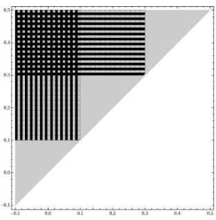
Figure 2 illustrates the idea behind these two axioms. Let S be the vertically striped region, R the checked region, and T the horizontally striped region. Assume all boundaries belong to R. Given a report of _ev = 0.1, the agents know that [a0, b0] ∈ S∪R. Similarly, given a report of ev = 0.3, the agents know [a

0_{, b}0_{]∈ R∪T. Our rst axiom requires that an}

agent prefers an asset with [a0, b0]∈ T to one with [a0, b0]∈ S. Our second axiom says that the agent must then prefer R∪T toS∪R. If the buyers satisfy these axioms,7 then a higher report to the market is always better news.

7_{A technical closure axiom guarantees that the checked regionRis not worse than the horizontally striped}

Figure 2: Preferences over sets of intervals. Thex-axis represents the ex post lower bounda0 on the asset's value. The y-axis represents the ex post upper bound b0. The gray triangle is the set of possible ranges of the seller's private information. The dominance axiom requires that agents prefer an asset with [a0, b0] in the horizontally striped region to one with [a0, b0]

in the vertically striped region. The betweenness axiom requires that adding the checked region to both the striped regions preserves the agents' preference ordering.

We therefore have the following:

Theorem 2.1 (Aggressive Reporting). If the seller's private information is [a0, b0], then the

uniquely optimal report is bv =b 0_.

2.3 Eects on demand

We now illustrate how Theorem 2.1 aects the bid distribution in the auction and leads to illiquidity. Because the seller can justify any value in [a0, b0], we require only that the reserve

price is in this range. Buyers, however, know only thatev ∈[a, b

0_{], which means that any bid}

above b0 is a dominated strategy. Bids below a are deliberate decisions to stay out of the auction. The region of interest is therefore[a, b0], in which buyers oer a bid that, from their

viewpoint, is potentially credible. See Figure 3.

Figure 3: Bids and reserve prices under mark-to-model. The seller optimally chooses a reserve price in [a0, b0]. A buyer who wishes to stay out of the market can bid anything in [0, a]. Because the seller optimally disclosesb0, no buyer with monotone preferences ever bids above b0. The buyers do not know a0, and therefore any buyers wishing to make a credible bid must choose a value in [a, b0].

from b0. If the highest bidder discounts the report below a0, then the market shuts down. Fixing the values of a andb0, it is easy to see that the higher a0 is, the greater the illiquidity from a given level of discounting. The reason is that the amount that the highest bidder discounts the report bv =b

0 _{can depend only on a and b}0_.8

A conservative reporting regime, in which the seller is required to report a0, shifts the range of credible bids to the right. Buyers wishing to make a credible bid in a conser-vative reporting regime choose a bid in [a0, b]. This interval is shifted to the right of the

corresponding interval under mark-to-model. The problem in choosing how to bid is also changed: rather than deciding on how much to discount the reported value, buyers must now decide how aggressively to bid above the reported value. A bid that is aboveb0which the buyers cannot estimategives the seller an information rent. For xed a0 and b , as b0 decreases, a buyer at a given level of aggressiveness in bidding will be more likely to pay the

8_{For a general overview in bidding on rst-price auctions with ambiguity, see Kaplan and Zamir (2015).}

Much of the research focuses on private value auctions, starting with Salo and Weber (1995) and the theory and experimental work of Chen et al. (2007). A common value auction, similar to our conservative reporting treatment, is in Dickhaut et al. (2011).

information rent, which cannot arise under mark-to-model. See Figure 4.

Figure 4: Bids and reserve prices under conservative reporting. The seller's reserve price is in [a0, b0]. A buyer who wishes to stay out of the market can bid anything in [0, a0]. The

buyers do not knowb0, and therefore any buyers wishing to make a credible bid must choose a value in[a0, b].

3 Description of the experiment and hypotheses

To test the predictions described in Section 2, we ran a laboratory experiment. We recruited participants from the Carnegie Mellon Tepper School of Business/Social and Decision Sci-ences participant pool, using an online recruiting program. The experiment was coded in z-Tree (Fischbacher, 2007).

Participants in the experiment were grouped together in groups of 5 for 16 rounds. Each group was assigned to one of three conditions: a discretionary reporting condition, an aggres-sive reporting condition, or a conservative reporting condition. The purpose of the discre-tionary condition was to test whether, given exibility in reporting, sellers of a nancial asset would report aggressively, as Theorem 2.1 predicts. The aggressive condition imposes the equilibrium strategy that the seller uses under fair value, in order to make the equilibrium report common knowledge. The conservative condition imposes the ex post lower bound

as the report. This structure enables us to separate our tests of the predicted reporting behavior from our tests of trading behavior under mark-to-model reporting. Both the dis-cretionary condition and the aggressive condition can be thought of as fair value treatments. We refer to the aggressive reporting condition henceforth as fair value, in order to emphasize that the discretionary treatment includes a reporting decision rather than starting with the equilibrium fair value report.

In each treatment, the computer privately and randomly selected one participant in each round as the seller for that round. The other four participants in the group were the buyers for that round. The choice of the seller in each round was made independently, from a discrete uniform distribution with replacement. The instructions explained the method of selecting the seller to the the participants. Keeping the participants grouped together enables us to rule out participant heterogeneity as the sole source of dierences in behavior across treatments. This is crucial to control for, as Ahn et al. (2014) demonstrate. However, grouping creates the possibility of order eects, in which behavior in one round aects decisions in subsequent rounds (e.g., learning, attempts at reputation building). We ran several tests for order eects, which we describe below in Subsection 4.6.

In each round, we endowed the seller with an asset which had a value commonly known to be between $0.50 and $1.50. We endowed the buyers with of $1.50, which they could use only in the current round. After the participants completed trading in a given round (as described below), the computer revealed the asset's value to all the participants, along with an indication of whether trade occurred and, if so, at what price. The computer deposited all the money that a participant held at the end of a given round into the participant's bank account, which determine the participant's earnings but was unavailable for trading in any subsequent round.

The setting of the experiment was a rst-price sealed bid auction, with a privately in-formed seller. The timeline, common to all treatments, follows Figure 1 from Section 2, with

a set to $0.50 and b to $1.50. In the conservative treatment, _bv was always set to a0. In the fair value treatment, bv was always set to b

0_{. The discretionary treatment allowed the seller}

to choose bv but required that bv ∈ [a

0_{, b}0_{]. The instructions explained the reporting to all}

participants.

To generate the values for (a0, v, b0) in each of the 16 rounds, we used the ambiguity

generator of Stecher et al. (2011). The procedure draws numbers from a nonstationary, nonergodic process, giving us a set of realizations for which each draw came from a new distribution, and for which the way the distribution changes between draws is unknowable. We partitioned the realizations into triples and sorted, making a0 the lowest realization in the triple, v the median realization, andb0 the highest.

In total, we generated ve blocks of 16 realized triples (a0, v, b0), and used a matched

pairs design. We ran one conservative session and one fair value session for each block of 16 triples, and ran two discretionary sessions using two of the blocks of realized triples.

Our main hypotheses, stated in alternative format, are as follow: H1

A: In the discretionary treatment, the distribution of reports rst-order stochastically

dominates the distribution of reserve prices. H2

A: The bid distribution in the conservative treatment rst-order stochastically dominates

the bid distribution in the fair value treatment.

H3_A: The maximum bid under conservative reporting is higher than the maximum bid under fair value.

H4

A: Fair value reduces liquidity. That is, Pr[trade| Fair Value]<Pr[trade |Conservative].

The rst hypothesis is based on Theorem 2.1. If sellers report aggressively, then they would disclose values that systematically exceed their reserve prices. The second and third hypotheses are related to demand and prices (or, if there is no trade, the latent price). H_A2

states that the overall level of demand is shifted downward under fair value compared with the conservative treatment. H3

Astates that the downward shift aects the highest bids, and

hence is signicant enough to aect prices in a rst-price auction. The last hypothesis states that fair value reporting reduces liquidity.9

Additionally, we test whether reserve prices are aected by the reporting regime, to rule out supply-driven factors, such as those discussed in Allen and Carletti (2008) and Plantin et al. (2008). We also conduct several robustness checks. For the results on liquidity, we test whether our repeated measures design drives the results. That is, we check whether dierences in liquidity across matched sessions could be driven by the same behavior of individual participants. For the results on the bid distribution, we test whether any shifts in demand are due to aggressive reporting being common knowledge. To do so, we compare the bid distributions of the discretionary sessions with those of the corresponding fair value and conservative sessions. To rule out order eects, we test whether reserve prices and maximum bids dier between the rst eight and the last eight rounds of the experiment.

4 Results

4.1 Participants

We recruited 60 participants for a total of twelve sessions. The median participant age was 24.5 years, with an interquartile range of 2129 years. Roughly 40% were female.

For the discretionary treatment, there were two groups of participants, giving 32 rounds of discretionary report and reserve price observations. For the conservative and fair value

9_{Because our data come from an experiment, we are able to observe latent prices, in the form of highest}

bids. Outside of the laboratory, an empiricist would be restricted to analyzing prices when trade occurs, possibly adding a selection equation. For this reason, we also tested hypothesisH3

Arestricting attention to rounds in which trade occurred. We found no dierences between focusing on prices or on latent prices. We choose to focus on latent prices here, in order to include all observations that address our hypotheses. The robustness of the results suggest that archival research with questions similar to ours would be unlikely to require a selection model to adjust for time periods without trade.

treatments, there were ve groups each, with each conservative group matched to a fair value group. In total, we had 80 matched pairs of rounds, with 160 reserve price observations and 640 bid observations.

Among the 80 matched pairs of conservative and fair value rounds, in 59 (74%), all par-ticipants in both groups made decisions that were rationalizable given an objective of prot maximization. In the remaining 21 rounds, at least one participant either made a bid that was guaranteed to lose money or chose a reserve price that was a dominated strategy. Among these violations of wealth maximization, 13 decisions were made by a single participant, who consistently bid more than the commonly known upper bound on the asset's value.10

Each session took approximately 45 minutes, including time to seat participants, read and quiz the participants on the instructions, and pay the participants at the end of the session. Earnings ranged from $19.60 to $24.02.

4.2 Result: discretion leads to aggressive reporting

In the two sessions with discretionary reporting, sellers provided both a reserve price and a report to the market. Because the private lower bound a0 and the private upper bound b0 varied across rounds, we calculate a normalized value bv−a

0

b0_−a0, representing how far the report b

v is along the line segment from a0 tob0. We use a similar normalization to scale the seller's reserve price v∗. Because the reserve price is chosen privately, it is a weakly dominant strategy for the seller to truthfully report v∗. If the seller's preferences are incomplete, as is commonly assumed in models with ambiguity (e.g., Bewley, 2002), then v∗ is optimally chosen at a value at which the seller is not worse o by selling and not better o by buying (see Appendix A). If the distribution ofbvrst-order stochastically dominates the distribution

of v∗, then there is evidence that the sellers report aggressively from their own viewpoint.

10_{To be complete, we perform our analyses in two ways: including all observations and focusing on those}

that are consistent with maximizing behavior. The results are robust to the inclusion or exclusion of the non-maximizing behavior, and we feel that remarking on both makes the analysis more complete.

Including this comparison is crucial, because it allows us to distinguish between aggressive reports and high reports arising from optimistic beliefs.

Figure 5 shows the cumulative empirical histograms of seller reserve prices and reported values. The x-axis gives the normalized distance along the line segment from a0 to b0. The y-axis shows the cumulative proportion of observations at or below a given level on the x -axis. The distribution of reports is shifted to the right of the distribution of reserve prices. The dierence between the cumulative distributions is signicant at the 0.05 level under a Kolmogorov-Smirnov test and at the 0.01 level under Anderson-Darling, Cramér-von Mises, and Mann-Whitney tests. We therefore strongly reject the null that the distribution of reports does not dominate that of reserve prices.

Figure 5: Cumulative distributions of scaled reported values (dark) and reserve prices (light) in baseline treatment.

In absolute terms, the median scaled reported value was 0.87, compared with a median scaled reserve price of 0.37. That is, the median report was roughly7/8of the distance along

the line segment from a0 to b0, while the median reserve price was only 3/8of this distance.

approximately at the upper boundb0. As is apparent from the gure, upper quartile of scaled reserve prices is considerably lower, at 0.82. Overall, the results support our hypothesisH1

A

that the discretionary treatment leads to aggressive reporting.

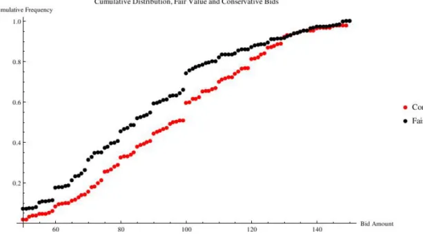
4.3 Results: bids and latent prices are lower under fair value

Given that discretion leads to aggressive reporting, we now address whether aggressive re-porting causes in a downward shift in demand, compared with conservative rere-porting. Fig-ure 6 shows the cumulative empirical histograms of bids in the conservative and fair value treatments. For the bid distributions, we do not scale the values between 0 and 1. The reason is that participants in the fair value treatment know the ex ante lower bound a and the ex post upper bound b0, whereas participants in the conservatism treatment know the ex post lower bound a0 and the ex ante upper bound b. The raw bid amounts are comparable, and the participants are matched across sessions, so unscaled data are more directly comparable. By contrast, the data in Figure 5 come from the sellers, who always know botha0 andb0, and in any case face the same information when choosing their reserve prices and their reports.

Figure 6 shows that the bid distribution under conservatism is to the right of the distri-bution under fair value. The dierence between the two empirical cumulative distridistri-butions is signicant at the 0.001 level under Anderson-Darling, Cramér-von Mises, Kolmogorov-Smirnov, and Mann-Whitney tests. This result supports our hypothesis H2

A that fair value

reporting lowers the amount buyers are willing to pay and thus weakens demand. Our third hypothesisH3

A addresses the fact that it is the the highest bid that determines

prices and liquidity, not the entire bid distribution. Table 1 compares the average values of the maximum bids across treatments, and shows the maximum bid was lower in the fair value treatment. Under a Wilcoxon signed-rank test, the dierence in the maximum bids was signicant at the 0.01 level. If we restrict attention to the rounds in which no participant chose a strictly dominated strategy, the dierence between bid distributions becomes more

Figure 6: CDFs of bids under the conservative and fair value reporting. signicant, with ap-value below 0.001. This supports our hypothesisH3

Athat bids are higher

under conservatism than under fair value.

Conservative Fair Value 112.8¢ 105.3¢

Table 1: Average value of highest bid across treatments

To test whether supply could also have played a role, we compared the distribution of reserve prices across treatments. Figure 7 shows the cumulative empirical histograms. The CDFs of reserve prices did not dier signicantly at any conventional levels. The p-values were 0.27, 0.30, 0.30, and 0.46, respectively, under the Kolmogorov-Smirnov, Cramér-von Mises, Anderson-Darling, and Wilcoxon signed-rank tests. We therefore fail to reject the null that reserve prices are independent of the reporting regime.

Combining these results, we nd that supply is not aected by the use of fair value, but demand is signicantly weakened. The lower prices are due to falling bids, reecting an increase in price eciency because of the disappearance of information rents. The falling

Figure 7: CDFs of reserve prices under conservative and fair value treatments. prices are not driven by seller behavior.

4.4 Result: fair value reduces liquidity

Having established that the fair value regime leads to aggressive reporting and weak de-mand, compared with a conservative regime, we now address whether fair value also causes illiquidity. Table 2 summarizes the frequency of trade under both regimes.

Conservative \ Fair Value Trade FV No Trade FV

Trade C 31.3% 36.3%

No Trade C 23.8% 8.8%

Table 2: Frequency of trade, cross tabulated across treatments.

An exact form of a McNemar test, which compares the o-diagonal entries with a binomial(80,1/2), gives a p-value of 0.0279 against a one-sided alternative.

To control for repeated measures, we use the two-step procedure of Eliasziw and Donner (1991). The rst step estimates the correlation among the discordant pairs (the o-diagonal elements in Table 2). The second step calculates an approximate McNemar test statistic,

adjusted for the estimated correlation.

The Eliasziw-Donner procedure gives an estimated correlation among discordant pairs of 0.183, which, though seemingly low, is enough to make the dierence in frequencies of discordant pairs insignicant. However, the correlation is driven almost entirely by a sin-gle participant, whose bids were above the commonly known upper bound in 13 rounds. Restricting attention to the 59/80 rounds consistent with wealth maximization makes the dierences in liquidity stronger and more signicant than under the ordinary McNemar test. The results are in Table 3.

Conservative \ Fair Value Trade FV No Trade FV

Trade C 30.5% 42.4%

No Trade C 15.3% 11.9%

Table 3: Frequency of trade, cross tabulated across treatments, consistent rounds only. Although the numbers in the cells of Tables 2 and 3 are similar, the Eliasziw-Donner correlation among discordant pairs changes dramatically, dropping to 0.048. The implication is that the participants who did not maximize wealth, and in particular the single participant who consistently made bids that were assured of losing money, generated almost the entire clustering eects. The dierence between the frequencies of discordant pairs in Table 3 is highly signicant, with a p-value of 0.009.

In practical terms, the dierence in trade frequency across treatments is quite large. From Table 3, trade occurred in 72.9% of rounds under the conservative treatment, compared with 45.8% of rounds under the fair value treatment. If we include the rounds with non-maximizing participants, trade occurs in 67.5% of rounds under conservatism versus 55.0% under fair value. The corresponding likelihood ratio is 1.59 for participants whose behavior is rationalizable and 1.23 overall. The results overall are consistent with our hypothesisH4

A

4.5 Robustness to failures of common knowledge of rationality

The analysis so far establishes a fair value regime lowers demand without aecting supply, compared with a conservative regime. This results in a drop in prices and in liquidity.

To test the robustness of our predictions, we look at bidding behavior in the discretionary treatment. This treatment is a more complex setting than the fair value treatment, because it requires participants to anticipate aggressive reporting from others, and adjust their bids accordingly. By contrast, in the fair value setting, all participants are informed that the reports will be aggressive. An initial analysis suggests that participants do not anticipate aggressive reporting from the sellers: in our discretionary sessions, we observed an astound-ingly high frequency of trade, occurring in 93% of the rounds! A more careful analysis, however, shows that the discretionary treatment is less anomalous than it initially seems.

Figure 8 shows the bid distribution in the discretionary sessions and the matched fair value and conservative reporting sessions. The bid distribution in the discretionary treatment is shifted leftward from the conservative treatment, though not as far leftward as the fair value treatment (in which the optimal aggressive report is imposed and commonly known). Consistent with the ndings of Malmendier and Shanthikumar (2007), Figure 8 shows that participants, when in the role of buyers, do not fully anticipate aggressive reporting, even though the same participants, when in the role of sellers, report aggressively. The driving force is the right tail of the bid distribution. The top quartile of bids are nearly identical under conservatism and under the discretionary treatment. Demand in general falls when moving from a conservative to a discretionary treatment, but the highest bid does not soften enough to eliminate trade.11 _{Even with the high frequency of trade in the}

discretionary treatment, the bids move in the predicted direction, and the same forces are in play as in our fair value sessions.

Figure 8: CDFs of reserve prices under all three treatments.

4.6 Robustness to order eects

Our design makes reputation building dicult, as the seller's identity is private, and a par-ticipant's expected number of times as a seller is only 3.2 rounds. Nevertheless, participants could anticipate repeated interaction, or could alter their decisions due to learning.

We conduct two tests of order eects. First, we check whether the reserve price distri-bution varied between the rst and last half of the experiment. Second, we check whether the highest bid varied in the rst and last half of the experiment. For the fair value groups, the dierence between reserve price distributions in the rst and last half of the experi-ment diered withp-values of 0.54, 0.59, 0.64, and 0.90, respectively, under Mann-Whitney, Anderson-Darling, Cramér-von Mises, and Kolmogorov-Smirnov tests. For the conservatism group, the corresponding p-values were 0.73, 0.91, 0.93, and 0.92. We therefore nd no evidence of an order eect on reserve prices.

Among the maximum bids, the p-values for dierences between the rst and last half of the experiment for the fair value group were 0.48, 0.56, 0.57, and 0.76, respectively, under

Mann-Whitney, Anderson-Darling, Cramér-von Mises, and Kolmogorov-Smirnov tests. For the conservatism group, the corresponding p-values were 0.29, 0.41, 0.37, and 0.40.

In sum, we nd no evidence of order eects in our participants' decisions.

5 Discussion and conclusion

Our analysis highlights the consequences of choosing between a conservative and a fair value reporting regime with mark-to-model reporting. We nd that a fair value regime leads to aggressive reporting, lower asset prices than under conservative reporting, and market illiquidity. These results are consistent with the theoretical results of Alchian (1977) and Lester et al. (2011, 2012), summarized in Lagos et al. (2015), who associate liquidity with the ease of recognizing an asset's quality. A conservative report makes a minimum quality known to market participants, avoiding a liquidity friction.

An important insight is that the lower asset prices under a fair value regime are not the result of the bursting of a bubble, but arise from the disappearance of information rents, which inate prices under a conservative regime. Lower prices under fair value reporting simply reects that the regime does what it is designed to do.

However, this gain in price eciency does not mean that fair value improves overall market eciency. Illiquidity under fair value is the result of a friction it generates, which is absent from a conservative regime. The tradeo is, therefore, between the information rents of a conservative regime and the illiquidity of a fair value regime.

Although evaluation of the consequences of illiquidity is beyond our scope, the macroeco-nomics literature suggests the impacts can be extremely large. Bernanke and Gertler (1989, 1990) and Bernanke et al. (1996, 1999) demonstrate the multiplier eect of liquidity frictions in lending markets; a good overview of this literature is in Hall (2010). Additionally, the ndings of Farmer (2015) suggest that a market collapse Granger causes unemployment, and

that the crash of the stock market played a major role in the severity of the Great Recession. To the extent that the stock market crash was linked to the evaporation of liquidity in the market for debt-backed securities, this would imply a drastic social cost of liquidity frictions. From a public policy viewpoint, it is natural to wonder if there is an easy x. Why not require rms to disclose both a conservative and a fair value estimate? This idea has established precedent in nancial reporting. For example, rms using LIFO to measure inventory ow also disclose in the notes to the nancial statements a LIFO reserve, which is calculated as if the rm had used FIFO. Reporting both a conservative and a fair value number would seem to give us a safeguard against illiquidity, while protecting investors against having to pay an information rent. But there is cause for skepticism.

The diculty is in assuring that rms would continue to disclose an aggressive fair value estimate when they are required to report a conservative valuation. A rm could be better o with a pessimistic mark-to-model estimate that simply restates the conservative valuation. Doing so enables the rm to disclose only the lower bound on its asset values, thereby retaining its information rent.

An alternative is to mandate explicitly that the rm provide a conservative and an aggressive estimate. Because one number would be declared to be aggressive, rms would no longer have incentive to underreport. The main concern associated with this approach is the additional costs of providing (and having audited) both a best-case and a worst-case scenario. Whether these costs are justiable depends on how large they are, compared with the costs of potential information rents. Future research studying this trade-o would provide useful information for standard setters and regulators.

A Axioms and Theoretical Development

The central tenet of our argument is that the discretion in mark-to-model accounting leads to aggressive reporting. In this appendix, we elaborate on the axioms on preferences that are necessary and sucient for aggressive reporting to be the seller's unique optimal reporting strategy. Because the market of interest to us is characterized by ambiguity, as discussed in Section 1, we allow preferences to be incomplete; see Bewley (2002) or the recent model of Easley and O'Hara (2010).

We require that all agents prefer an asset that is guaranteed to have a higher value to one that is guaranteed to be lower. Letting

X ={[a, b]|a ≤a≤b≤b},

we have the following.

Axiom A.1 (Interval Order). All agents have preferences that are monotone in the range of values, in the interval order sense of Fishburn (1985): if asset x has value in [a, b] and

asset y has value in [c, d], then

b≤c⇒x_-y,

and if there is at least one strict inequality among a ≤b≤c≤d, then x≺y.

For convenience, we will write preferences as if directly on X. Thus, we will henceforth write [a, b] _-[c, d] instead of writing x_-y for asset x with values in [a, b] and asset y with values in [c, d].

Violations of Axiom A.1 lead to counterexamples to the unique optimality of always reporting the private upper bound. If buyers have a bliss point, then there is nothing to be gained by reporting that a value above the bliss point is feasible. Note that A.1 implies a full support condition.

Because a report bv is feasible if and only if a 0 _≤

b

v ≤ b0, buyers learn from the seller's report that a0 ∈[a,_bv] and b0 ∈[_bv, b]. We therefore extend preferences to rectangular subsets

of X (rectangles), which are sets of the form

R(w, x, y, z) := {[a, b]∈X|w≤a≤x≤y≤b≤z}.

In this notation, the report bv is feasible if and only if[a

0_{, b}0_{] is in the rectangleR(a,} b

v,_bv, b).

Our next axiom is monotonicity with rectangular sets.

Axiom A.2 (Witnessed Strict Dominance). LetS, T be nonempty rectangular subsets of X. Suppose that

(∀[a0, b0]∈S)(∃[a00, b00]∈T) [a0, b0]≺[a00, b00]

and

(∀[c00, d00]∈T)(∀[c0, d0]∈S) ¬([c00, d00]_-[c0, d0]).

Then S ≺T.

A.2 is weaker than strict dominance. It says that, if every element of S is strictly dominated by something in T, and nothing in T is strictly dominated by anything in S, then S ≺ T. That is, given a possible range of values in S, there must be a witness in T willing to testify thatT oers something better. If this condition holds, then the agent must prefer T to S. Referring Figure 2, Axiom A.2 requires that the horizontally striped region, excluding the left boundary, is strictly better than the vertically striped region, excluding the top boundary. If this does not hold, and our next axiom does, then the seller would be better o issuing a lower report than an higher report.

Axiom A.2 compares regions that are feasible under one report and infeasible under another. That is, A.2 addresses the symmetric dierence of feasible regions for distinct reports. The next axiom, which we call disjoint union betweenness, compares the intersection

of feasible regions.

Axiom A.3 (Disjoint Union Betweenness). Let S, T, U be nonempty rectangular subsets of X. Suppose S ≺T, ¬(U ≺S), and ¬(T ≺U). Then

U ∪S ≺U∪T.

It is important to restrict attention to rectangles that are no worse than a preferred rectangle and no better than the dominated rectangle. To see why, assume S≺T and U, S, and T are pairwise disjoint. Suppose U ≺ S, and that T is a small region, say a single identied point [v, v]. Suppose U is a larger region than T, but a much smaller region than S. ThenU ∪T is almost identical to U, andU ∪S is almost identical to S. The restriction of Axiom A.3 to regions U that are not worse than S or better than T avoids this diculty. Although violations of Axioms A.1A.3 can provide examples in which aggressive re-porting is not uniquely optimal, these axioms alone are insucient to guarantee aggressive reporting. The reason is that none of Axioms A.1A.3 assures that the checked region in Figure 2 is neither better than the horizontally striped region nor worse than the vertically striped region. The additional axiom we needs is a closure condition. We rst dene a notion of distance.

Denition A.1. Let [a, b],[a0, b0]∈X, and let U ⊆X. Dene d([a, b],[a0, b0]) := k(a, b)−(a0, b0)k d([a, b], U) := inf [a00_,b00_]∈Ud([a, b],[a 00 , b00]) If U =_∅, then set d([a, b], U) :=−∞.

R2, as in Figure 2. Dene the distance between two intervals be the Euclidean distance

between the associated points in R2, and let the distance from an interval [a, b] ∈ X to a

subset U ⊆X be the distance from [a, b]to the closest point in X.

Axiom A.4 (Closure). Let S, T be rectangular subsets of X, with S ≺ T. Then for all

[a, b],[a0, b0]∈X, if d([a, b], S) = d([a0, b0], T) = 0, {[a, b]}_-{[a0, b0]}.

Lastly, we impose a consistency condition.

Axiom A.5 (Consistency). Let S, T ⊆ X. Suppose (∀[a, b] ∈ S)(∀[c, d] ∈ T), we have [a, b]_-[c, d]. Then S _-T.

Lemma A.6. Let a < v0 < v00< b. Dene the rectangles

S = R(a, v0, v0, v00)\{[a, b]∈X|a≤a≤v0 and b =v00} T = R(v0, v00, v00, b)\{[a, b]∈X|a=v0 and v00 ≤b ≤b} U = R(a, v0, v00, b)

Then ¬(U ≺S) and ¬(T ≺U).

Remark. In Lemma A.6, the regions S, T, and U correspond to the vertically striped, hori-zontally striped, and checked regions in Figure 2.

Proof. First, note that, for every [a0, b0] ∈ S with a0 < v0, the points {[a, b] ∈ X|a =

v0 and v00 ≤b ≤b} ⊂U strictly dominate [a0, b0]. On the other hand, no point in S strictly dominates any point in U. So again by witnessed strict dominance,S\{[a, b]∈S|a=v0} ≺ U.

Next, observe that for any[v0, b]∈Sand any[c, d]∈U, we haved([v0, b], S) = d([c, d], U) = 0. So by the closure axiom A.4, [v0, b] _- [c, d]. We therefore have, for all [a, b] ∈ S and for all[c, d]∈U, [a, b]_-[c, d], and hence by the consistency axiom A.5, S _-U.

We can now prove Theorem 2.1.

Proof of Theorem 2.1. Let S, T, U be as in the proof of Lemma A.6. We will show that S∪U ≺T ∪U. Since S∪U is the information the buyer receive from reportv0 and T∪U is the information the buyers receives from report v00> v0, it then follows that a higher report is always better news. Consequently, the seller's uniquely optimal strategy is to choose the highest admissible report, bv =b

0_.

Observe that S ≺ T; this is an immediate consequence of the interval order axiom A.1 and the witnessed strict dominance axiom A.2. Lemma A.6 then guarantees that S _- U and U _-T. By the disjoint union betweenness axiom A.3, the result follows.

B Instructions

We provide the instructions and the review questions for the conservative treatment. The instructions for other treatments are shown in brackets.

Instructions

This is an experiment in the economics of decision-making. This experiment will last approximately one hour. Do not talk to others at any time during the experiment. If you have any questions during the experiment, please raise your hand.

To make a prot, you will trade a nancial asset. At the end of the experiment, we will pay you a show-up fee of $5 plus any prots you will have made.

The experiment will last for 16 rounds. In each round, the computer will randomly select one person as the seller. The other four participants will be buyers for that round. Everyone has an equal chance of being the seller in any given round. The computer will tell you whether you are a seller or a buyer. The computer will not tell the buyers who the seller is. At the beginning of each round, the seller will receive an asset, and the buyers will receive 150 cents. The computer will determine the asset's value at the end of the round.

Your Information [Discretionary treatment: Your Information and the Seller's Report] If you are the seller, the computer will tell you a minimum and maximum value of the asset for that round. The minimum will be at least 50 cents, and the maximum will be at most 150 cents. The asset's value will be between the minimum and maximum. [Discretionary treatment: The computer will ask you to enter a possible value of the asset, which must be between the minimum and the maximum.] If you are a buyer, the computer will tell you the minimum, and will remind you that maximum is at most 150 cents. [Fair value treatment: If you are a buyer, the computer will tell you the maximum, and will remind you that minimum is at least 50 cents.] [Discretionary treatment: If you are a buyer, the computer will tell you the possible value the seller entered.]

The Auction

If you are a seller, the computer will ask you to enter the lowest price for which you are willing to sell the asset. None of the buyers will see the minimum price you enter.

If you are a buyer, the computer will ask you to enter the amount you are willing to pay for the asset. We call this amount your bid. You may enter any amount from 0 to your 150 cents. None of the other participants will see your bid.

If the highest bid is at least the minimum price the seller is willing to accept, then the computer will sell the asset to the buyer who made the highest bid. The price will be the amount of the highest bid. If two or more buyers tie for the highest bid, then the computer will randomly select one of these buyers and sell the asset to the selected buyer. The computer will then determine the asset's value. If trade does not occur, the seller will receive the asset's value. If trade occurs, the buyer who bought the asset will receive the asset's value. After the computer determines the asset's value, your money for the current round will be deposited into your account.

At the end of the experiment, we will pay you the balance in your account. If your account balance is negative, we will still pay you the full $5 show-up fee.

If you have any questions, please raise your hand now. Review Questions

Please answer the following questions. Your answers will not aect your payment. 1. The computer tells the seller that the asset is at least 59 cents and at most 120 cents.

The computer will also tell the buyer that the asset is worth at most 120 cents. [Dis-cretionary Treatment: The computer tells the seller that the asset is worth at least 59 cents and at most 120 cents. The computer will also tell the buyers the possible value the seller enters.]

True False

2. The computer tells the seller that the asset is at least 59 cents and at most 120 cents. The computer will also tell the buyer that the asset is worth at least 59 cents. [Dis-cretionary treatment: The computer tells the seller that the asset is worth at least 59 cents and at most 120 cents. The seller may enter a possible value of 125 cents.]

True False

3. The lowest price for which the seller is willing to sell the asset is 76 cents. The highest bid is 87 cents. Trade will occur.

True False

4. The lowest price for which the seller is willing to sell the asset is 87 cents. The highest bid is 76 cents. Trade will occur.

References

D. Ahn, S. Choi, D. Gale, and S. Kariv. Estimating ambiguity aversion in a portfolio choice experiment. Quantitative Economics, 5(2):195223, 2014.

N. I. Al-Najjar. Decision makers as statisticians: Diversity, ambiguity, and learning. Econo-metrica, 77(5):13711401, 2009.

A. A. Alchian. Why money? Journal of Money, Credit and Banking, 9(1):133140, 1977. F. Allen and E. Carletti. Mark-to-market accounting and liquidity pricing. Journal of

Accounting and Economics, 45(23):358378, 2008.

H. Arló-Costa and J. Helzner. Ambiguity aversion: the explanatory power of indeterminate probabilities. Synthese, 172(1):3755, 2010.

R. J. Aumann. Utility theory without the completeness axiom. Econometrica, 30:445462, 1962.

R. J. Aumann. Utility theory without the completeness axiom: A correction. Econometrica, 32(1/2):210212, 1964.

A. Beatty and J. Weber. Accounting discretion in fair value estimates: An examination of SFAS 142 goodwill impairments. Journal of Accounting Research, 44(2):257288, 2006. B. Bernanke and M. Gertler. Agency costs, net worth, and business uctuations. American

Economic Review, 79(1):1431, 1989.

B. Bernanke and M. Gertler. Financial fragility and economic performance. Quarterly Journal of Economics, 105(1):87114, 1990.

B. Bernanke, M. Gertler, and S. Gilchrist. The nancial accelerator and the ight to quality. Review of Economic Studies, 78(1):115, 1996.

B. S. Bernanke, M. Gertler, and S. Gilchrist. The nancial accelerator in a quantitative business cycle framework. In J. B. Taylor and M. Woodford, editors, Handbook of Macroe-conomics, volume 1, pages 13411393. Elsevier, 1999.

T. F. Bewley. Knightian decision theory. Part I. Decisions in Economics and Finance, 25 (2):79110, 2002.

W. G. Blacconiere, J. R. Frederickson, M. F. Johnson, and M. F. Lewis. Are voluntary disclosures that disavow the reliability of mandated fair value information informative or opportunistic? Journal of Accounting and Economics, 52(23):235251, 2011.

K. P. Bogart. An obvious proof of Fishburn's interval order theorem. Discrete Mathematics, 118(13):239242, 1993.

E. D. Bolker. A simultaneous axiomatization of utility and subjective probability. Philosophy of Science, 34(4):333340, 1967.

B. Bratten, L. M. Gaynor, L. McDaniel, N. R. Montague, and G. E. Sierra. The audit of fair values and other estimates: The eects of underlying environmental, task, and auditor-specic factors. Auditing: A Journal of Practice and Theory, 32(Supplement 1): 744, 2013.

D. S. Bridges and G. B. Mehta. Representations of Preference Orderings, volume 422 of Lecture Notes in Economics and Mathematical Systems. Springer-Verlag, 1995.

J. Broome. Bolker-Jerey expected utility and axiomatic utilitarianism. Review of Economic Studies, 57(3):477502, 1990.

M. K. Brunnermeier. Deciphering the liquidity and credit crunch 20072008. Journal of Economic Perspectives, 23(1):77100, 2009.

Y. Chen, P. Katu²cák, and E. Ozdenorenc. Sealed bid auctions with ambiguity: Theory and experiments. Journal of Economic Theory, 136(1):513535, 2007.

S. Choi, L. Nesheim, and I. Rasul. Reserve price eects in auctions: Estimates from multiple RD designs. Economic Inquiry, Forthcoming, 2015.

J. Coval, J. Jurek, and E. Staord. The economics of structured nance. Journal of Economic Perspectives, 23(1):325, 2009.

P. M. Dechow, L. A. Myers, and C. Shakespeare. Fair value accounting and gains from asset securitizations: A convenient earnings management tool with compensation side-benets. Journal of Accounting and Economics, 49(12):225, 2010.

J. Dickhaut, R. Lunawat, K. Pronin, and J. Stecher. Decision making and trade without probabilities. Economic Theory, 48(2-3):275288, 2011.

J. Dubra, F. Maccheroni, and E. A. Ok. Expected utility theory without the completeness axiom. Journal of Economic Theory, 115(4):118133, 2004.

D. Easley and M. O'Hara. Liquidity and valuation in an uncertain world. Journal of Financial Economics, 97(1):111, 2010.

M. Eliasziw and A. Donner. Application of the McNemar test to non-independent matched pair data. Statistics in Medicine, 10(12):19811991, 1991.

P. Embrechts, G. Puccetti, and L. Rüschendorf. Model uncertainty and VaR aggregation. Journal of Banking & Finance, 37(8):27502764, 2013.

E. Eyster and G. Weizsäcker. Correlation neglect in nancial decision making. Discussion Paper 1104, DIW Berlin, February 2011.

R. E. A. Farmer. The stock market crash really did cause the great recession. Oxford Bulletin of Economics and Statistics, Forthcoming, 2015.

U. Fischbacher. z-Tree: Zurich toolbox for ready-made economic experiments. Experimental Economics, 10(2):171178, 2007.

P. C. Fishburn. Interval Orders and Interval Graphs: A Study of Partially Ordered Sets. Wiley, 1985.

R. Forsythe, R. Lundholm, and T. Rietz. Cheap talk, fraud, and adverse selection in nancial markets: Some experimental evidence. Review of Financial Studies, 12(3):481518, 1999. I. Gilboa and D. Schmeidler. Maxmin expected utility with non-unique prior. Journal of

Mathematical Economics, 18(2):141153, 1989.

B. W. Goh, J. Ng, and K. O. Yong. Market pricing of banks' fair value assets reported under SFAS 157 during the 2008 economic crisis. Working paper, Singapore Management University, 2009.

R. E. Hall. Why does the economy fall to pieces after a nancial crisis? Journal of Economic Perspectives, 24(4):320, 2010.

T. R. Kaplan and S. Zamir. Advances in auctions. In Handbook of Game Theory with Economic Applications, volume 4, chapter 7, pages 381453. Elsevier, 2015.

U. Khan. Does fair value accounting contribute to systemic risk in the banking system? Working paper, Columbia University, 2012.

R. R. King and D. E. Wallin. Voluntary disclosures when seller's level of information is unknown. Journal of Accounting Research, 29(1):96108, 1991.

P. Klibano, M. Marinacci, and S. Mukerji. A smooth model of decision making under ambiguity. Econometrica, 73(6):18491892, 2005.

R. Lagos, G. Rocheteau, and R. Wright. The art of monetary theory: A new monetarist perspective. Journal of Economic Literature, Forthcoming, 2015.

C. Laux and C. Leuz. Did fair-value accounting contribute to the nancial crisis? Journal of Economic Perspectives, 24(1):93118, 2010.

V. Lei, C. N. Noussair, and C. R. Plott. Nonspeculative bubbles in experimental asset markets: Lack of common knowledge of rationality vs. actual irrationality. Econometrica, 69(4):831859, 2001.

B. Lester, A. Postlewaite, and R. Wright. Information and liquidity. Journal of Money, Credit and Banking, 43(Supplement 2):355377, 2011.

B. Lester, A. Postlewaite, and R. Wright. Information, liquidity, asset prices, and monetary policy. Review of Economic Studies, 79(3):12091238, 2012.

F. Maccheroni, M. Marinacci, and A. Rustichini. Ambiguity aversion, robustness, and the variational representation of preferences. Econometrica, 74(6):14471498, 2006.

M. Magnan, A. Menini, and A. Parbonetti. Fair value accounting: Information or confusion for nancial markets? Review of Accounting Studies, 20(1):559591, 2015.

U. Malmendier and D. Shanthikumar. Are small investors naive about incentives? Journal of Financial Economics, 85(2):457489, 2007.

P. Manzini and M. Mariotti. On the representation of incomplete preferences over risky alternatives. Theory and Decision, 65(4):303323, 2008.

M. Öztürk and A. Tsoukiàs. Preference representation with 3-point intervals. In G. Brewka, S. Coradeschi, A. Perini, and P. Traverso, editors, Proceedings of the 17th European

Con-ference on Articial Intelligence (ECAI 2006), volume 141 of Frontiers in Articial Intel-ligence, pages 417421, 2006.

G. Plantin, H. Sapra, and H. S. Shin. Marking-to-market: Panacea or Pandora's box? Journal of Accounting Research, 46(2):435460, 2008.

A. A. Salo and M. Weber. Ambiguity aversion in rst-price sealed-bid auctions. Journal of Risk and Uncertainty, 11(2):123137, 1995.

H. Sapra. Do accounting measurement regimes matter? A discussion of mark-to-market accounting and liquidity pricing. Journal of Accounting and Economics, 45(23):379387, 2008.

M. Schmidt. Fair value: Your value or mine? An observation on the ambiguity of the fair value notion illustrated by the credit crunch. Accounting in Europe, 6(2):271282, 2009. H. S. Shin. News management and the value of rms. RAND Journal of Economics, 25(1):

5871, 1994.

C. J. Song, W. B. Thomas, and H. Yi. Value relevance of FAS No. 157 fair value hierarchy information and the impact of corporate governance mechanisms. The Accounting Review, 85(4):13571410, 2010.

J. Stecher, T. Shields, and J. Dickhaut. Generating ambiguity in the laboratory. Management Science, 57(4):705712, 2011.

J. D. Stecher. Existence of approximate social welfare. Social Choice and Welfare, 30(1): 4356, 2008.

K. Steele. Distinguishing indeterminate belief from risk-averse preferences. Synthese, 158 (2):189205, 2007.