A novel optimal PID plus second order derivative controller for AVR system

Full length article

A novel optimal PID plus second order derivative controller

for AVR system

Mouayad A. Sahib

Software Engineering Department, Salahaddin University, Kurdistan Regional, Erbil, Iraq

a r t i c l e i n f o

Article history:

Received 6 August 2014 Received in revised form 7 November 2014 Accepted 19 November 2014 Available online 6 January 2015 Keywords:

Optimal control PID controller

Automatic voltage regulator Particle swarm optimization Fractional order PID

a b s t r a c t

This paper proposes a novel controller for automatic voltage regulator (AVR) system. The controller is a four term control type consisting of proportional, integral, derivative, and second order derivative terms (PIDD2). The four parameters of the proposed controller are optimized using particle swarm optimization (PSO) algorithm. The performance of the proposed PIDD2is compared with various PID controllers tuned by modern heuristic optimization algorithms. In addition, a comparison with the fractional order PID (FOPID) controller tuned by Chaotic Ant Swarm (CAS) algorithm is also performed. Furthermore, a fre-quency response, zero-pole map, and robustness analysis of the AVR system with PIDD2is performed. Practical implementation issues of the proposed controller are also addressed. Simulation results showed a superior response performance of the PIDD2controller in comparison to PID and FOPID controllers. Moreover, the proposed PIDD2 can highly improve the system robustness with respect to model uncertainties.

©2014 Karabuk University. Production and hosting by Elsevier B.V. This is an open access article under the CC BY-NC-ND license (http://creativecommons.org/licenses/by-nc-nd/3.0/).

1. Introduction

In power generation systems, automatic voltage regulator (AVR) is utilized to maintain the terminal voltage of a synchronous generator at a specified level. The AVR controls the consistency of the terminal voltage by varying the exciter voltage of the generator

[1]. Due to the high inductance of the generatorfield windings and load variation, stable and fast response of the regulator is difficult to achieve. Therefore, it is important to improve the AVR performance and ensure stable and ef_ficient response to transient changes in terminal voltage. Various control structures have been proposed for the AVR system, however, among these controllers the proportional plus integral plus derivative (PID) was the most preferable controller. The PID controller is distinguished by its robust perfor-mance over a wide range of operating conditions and simplicity of structure design[2]. The design of the PID controller involves the determination of three parameters which are the proportional, integral, and derivative gains. In recent years, many intelligent optimization algorithms were proposed to tune the PID gains of the AVR system. Such algorithms include Particle Swarm Optimization (PSO) [3], Genetic algorithm (GA) [3,4], Craziness based particle

swarm optimization (CRPSO)[5], Reinforcement Learning Autom-ata (RLA)[6], Artificial Bee Colony (ABC)[7], Differential Evolution Algorithm (DEA)[8], Many Optimizing Liaisons (MOL) [9], Local Unimodal Sampling (LUS)[10], and Chaotic Ant Swarm (CAS)[11]. CAS is a new search algorithm inspired by the biological behavior of ants in nature proposed by Li et al.[12]. However, it is a deter-ministic process different from the conventional ant algorithm[13]. It combines the chaotic behavior of individual ants with the intel-ligent optimization action of an ant colony and thus it integrates the advantages of chaotic search and the powerful ability of swarm collectiveness. Based on CAS algorithm, Li et al. developed a model which can be used to describe how an ant colony organizes itself to find the optimal path between a food source and the nest[14]. The CAS algorithm shows a great potential in solving difficult optimi-zation problems encountered in variousfields such as parameter identification of dynamic systems[13], fuzzy system identification

[15], and parameters tuning of PID controller[11].

Recently, large and growing body of literature has investigated the concept of fractional calculus in many control applications to enhance the performance of PID controller[16e18]. Fractional or-der PID (FOPID) controller wasfirst proposed by Podlubny in 1999

[19]. FOPID is a generalization of the PID in which the orders of derivatives and integrals are non-integer[20]. The application of FOPID controller was also employed to control AVR system[21e23]. Compared to conventional PID, FOPID can ensure good control

E-mail address:[email protected].

Peer review under responsibility of Karabuk University.

H O S T E D BY Contents lists available atScienceDirect

Engineering Science and Technology,

an International Journal

j o u r n a l h o m e p a g e :h t t p : / / w w w . e l s e v i e r . c o m / l o c a t e / j e s t c h

http://dx.doi.org/10.1016/j.jestch.2014.11.006

2215-0986/©2014 Karabuk University. Production and hosting by Elsevier B.V. This is an open access article under the CC BY-NC-ND license (http://creativecommons.org/ licenses/by-nc-nd/3.0/).

performance and improve the system robustness with respect to model uncertainties[24]. However, due to fractional order in the differentiator and integrator, realization of FOPID is performed with high order discrete time controllers affecting the computational load and memory size of the control algorithm. Therefore, various approximation methods have been proposed to reduce the con-troller's order. However, the so-called long memory principle feature of the FOPID controllers will not be preserved after approximation. Another property that is lost after approximation is the optimality of controller[25].

The main contribution of this paper is to propose a novel four term structure PID plus second order derivative (PIDD2) controller for AVR system. The four gains of the PIDD2are tuned by PSO al-gorithm. The performance of the proposed PIDD2_{is compared with}

some PID controllers tuned by recently published modern heuristic optimization algorithms such as MOL, GA, ABC, DEA, and LUS al-gorithms. In addition, a comparison with the FOPID controller tuned by CAS algorithm is also performed. The performance of the proposed PIDD2is further investigated using frequency response, zero-pole map, and robustness analysis.

The remaining part of this paper is organized as follows. In Section2, the AVR system model is described. The AVR system with PID controller is analyzed in Section 3. The proposed PIDD2 controller is presented in Section4. The PSO algorithm is explained in section5. In Section6, the practical implementation issues of the PIDD2controller are addressed. Section7is devoted to computer simulation. Finally, Section8concludes the paper.

2. AVR system model

In synchronous generators, the AVR system is used to maintain the terminal voltage magnitude at a constant specified level. A simple AVR system consists of four main components, namely amplifier, exciter, generator, and sensor. Each component is modeled by afirst order system defined by a gain and a time constant.Table 1, shows the four AVR main components transfer functions with their corresponding gain and time constants typical ranges[9].

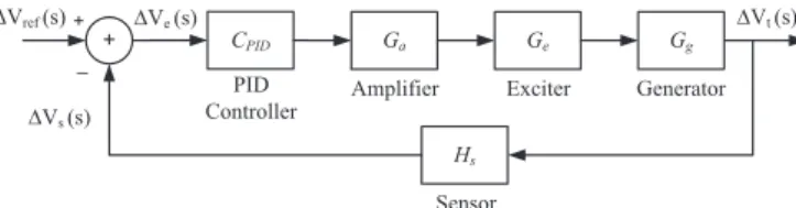
The arrangement of the AVR system components is shown in

Fig. 1. The terminal voltage

D

Vt(s) of the generator is continuously sensed by the sensor and compared with the desired reference voltage

D

Vref(s). The difference between the reference and the

sensed terminal voltages (error voltage

D

Ve(s)) is amplified through the amplifier and used to excite the generator using the exciter. The

AVR system parameters considered in this work are; Ka¼10.0,

Ta¼0.1, Ke¼1.0, Te¼0.4, Kg¼1.0, Tg¼1.0, Ks¼1.0, Ts¼0.01

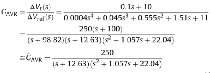
[3,7,9,24,26]. With these parameter values the closed loop transfer function of the AVR system becomes:

G_AVR¼ DVtðsÞ DVrefðsÞ ¼ 0:1sþ10 0:0004s4_þ0:045s3_þ0:555s2_þ1:51sþ11 ¼ 250ðsþ100Þ ðsþ98:82Þðsþ12:63Þs2þ1:057sþ22:04 yG~_AVR¼ 250 ðsþ12:63Þs2þ1:057sþ22:04 (1)

The transfer function of the AVR system (GAVR) have one zero at z¼ 100, two real poles ats1¼ 98.82 ands2¼ 12.63, and two

complex poles ats3,4¼ 0.53± 4.66i. TheGAVRcan be

approxi-mated by canceling the zero at100 with the pole at98.82 to obtainG~AVR. The unit step responses ofGAVRandG~AVRare shown in Fig. 2. It can be observed from Fig. 2that the AVR system GAVR

and its approximation G~AVR are almost similar and possess an

underdamped response with steady state amplitude value of 0.909, peak amplitude of 1.5 (Mp ¼ 65.43%) at tp ¼ 0.75, tr ¼0.42 s,

ts¼6.97 s at which the response has settled to 98% of the steady state value.

3. Analysis of the AVR system with PID controller

The response of the AVR can be improved by utilizing a controller in the forward path capable of processing the voltage difference

D

Ve(s) and producing a manipulated actuating signal. Commonly, a PID controller is employed for this task due to its simple structure. The PID controller combines three control actions related to the error signal in proportional, deferential, and integral manners and its transfer function is given by:

CPID¼KpþK_siþsKd (2)

whereKp,Ki, andKdare the proportional, integral, and derivative gains, Fig. 3shows a block diagram of the AVR system with PID controller. The general transfer function of the AVR system controlled by a PID controller is given by

GAVR_PID¼

CPIDGaGeGg

1þCPIDGaGeGgHs (3)

Table 1

Transfer functions of the AVR system components.

AVR component Transfer function Range of the gainK Range of the time constantT(s) Amplifier Ga¼ Ka Tasþ1 10e40 0.02e0.1 Exciter Ge¼ Ke Tesþ1 1e10 0.4e1.0 Generator _Gg¼ Kg Tgsþ1 0.7e1 1.0e2.0 Sensor Hs¼ Ks Tssþ1 0.9e1.1 0.001e0.06

Fig. 1.AVR system block diagram.

0 2 4 6 8 10 12 0 0.2 0.4 0.6 0.8 1 1.2 1.4 1.6 Step Response Time (seconds) A m plit ud e G_AVR G_AVRm

Substituting the transfer functions of the AVR system components listed inTable 1with their parameters and the transfer function of the PID controller given by Equation(2)in(3)yields,

The effect of the PID gain parameters on the overall AVR system can be analyzed by plotting the closed loop zero-pole locus as a function of the PID gains. The zero-pole locus can be obtained when

Kp,Ki, andKdare varied within the closed ranges 1KpKp_max,

0KiKi_max, and 0KdKd_maxrespectively. The initial state of

the zero-pole locus can be easily obtained by settingKp¼1,Ki¼0,

andKd¼0 in Equation(4)and as a result the transfer function of the AVR system reduces to that given by Equation(1)(without PID controller).

The characteristic of the transient response of the AVR system is closely related to the location of the closed-loop poles. From the design viewpoint, the adjustment of the PID gains may move the closed-loop poles to a desired location. Hence, with the use of the zero-pole locus method, it is possible to determine the values of the PID gains that will make the damping ratio of the domi-nant closed-loop poles as prescribed. However, a multi-gain root-locus is not an easy way to obtain and dif_ficult to illustrate and plot on the complex plane. Alternatively, the problem of

evaluating the optimum PID gains can be handled using an optimization problem in which an optimization algorithm is employed. The optimization algorithm, such as PSO, uses an

objective or cost function to tune the PID gains. For example, Panda et al., proposed the simplified PSO algorithm to design a PID controller for the AVR system[9]. By investigating the zero-pole map of the overall transfer function (the AVR system with the designed PID), given by[9],

one can observe that the objective of the PID controller is to compensate the effect of two poles in the AVR system at s1 ¼ 2.11 and s2 ¼ 1.06, thus the overall transfer

function GAVRPID can be approximated to G~AVRPID. Fig. 4, shows

the step responses ofGAVRPID andG~AVRPID.

FromFig. 4, it is observable that the step response of the AVR system and its approximation has been improved when using an optimal PID controller. This is evident through an improved values of rise timetr¼ 0.343, settling time ts ¼ 0.516 sec, maximum overshootMp¼1.95%, and damping ratio

z

¼0.72.

From the above analysis, it can be concluded that the PID controller attempts to compensate the effect of two poles of the AVR system. When the PID controller gain parameters are optimized, the overall transfer function is approximately reduced from fourth to a simple second order system. However, in a second-order system, the maximum overshoot and the rise time of the unit step response conflict with each other. Therefore, the improvement of the AVR system response achieved by the conventional PID controller is a compromise between maximum overshoot and rise time.

4. PID plus second order derivative controller (PIDD2₎

The closed loop transfer function of the AVR system with opti-mized PID controller can be approximated by a standard form of a second-order system given by

~ GAVRPID¼ u2 n s2_þ2zunsþu2 n (6)

where

un

is the undamped natural frequency. The proposed method is to modify the structure of the conventional PID controller such that it can reduce the overall transfer function to produce a modi_fied form of Equation(6)in which an additional zero is added ats¼

a

, such that,

Gz¼ s aþ1 u2 n s2_þ2zunsþu2 n ¼s

aG~AVRPIDþG~AVRPID (7)

0 0.2 0.4 0.6 0.8 1 1.2 1.4 0 0.2 0.4 0.6 0.8 1 1.2 1.4 Time (seconds) Amplitude G_{AVR PID}

G_{AVR PID} (approximated)

Fig. 4.Step response of the AVR system with PID controller.

GAVR_PID¼ 0:1Kds3þ 0:1Kpþ10Kd s2_þ0:1K iþ10Kpsþ10Ki 0:0004s5_þ0:0454s4_þ0:555s3_{þ ð1:51þ10K} dÞs2þ 1þ10Kp sþ10K_i (4) G_AVR PID¼ 0:01772s3_þ1:831s2_{þ5:899sþ4:189} 0:0004s5þ0:045s4þ0:555s3þ3:282s2þ6:857sþ4:189 ¼ 44:3ðsþ100:03Þðsþ2:26Þðsþ1:05Þ ðsþ100:49Þðsþ2:11Þðsþ1:06Þs2þ9:84sþ46:52y ~ G_AVR PID¼ 46:52 s2þ9:84sþ46:52; (5)

then the step response of the modified system become Yz¼1_sGz¼1_s

_s

aG~AVRPIDþG~AVRPID

¼s a 1 sG~AVRPID þ 1 sG~AVRPID (8)

where ð1=sG~AVRPIDÞis the unit step response (Y) of the original

approximated transfer functionðG~AVRPIDÞ, thus,

Yz¼s

aYþY or yzðtÞ ¼

1

ay_ðtÞ þyðtÞ (9)

This means that, the step response of the modified second order system with a zero ats¼

a

is given by the step response of the original system plus a scaled version of its derivative. As the zero moves further to the left side of the complex plane (

a

increases), the contribution of the derivative termy_ðtÞdecreases and the step response of the modified system starts to resemble the response of the original approximated system. Conversely, as the zero moves closer to the origin from the left side (

a

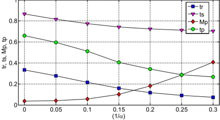
decreases), the contribution of the derivative term y_ðtÞ increases resulting in an increased overshoot, decreased rise and peak times (the step response be-comes faster). Fig. 5, shows the effect of adding a zero to the approximated system defined by Equation (5) on the unit step response. The scaling factor (1/

a

) of the derivative term y_ðtÞis varied from 0 to 0.3.

FromFig. 5, it can be observed that when the contribution of the derivative term increases (1/

a

increases) the response becomes faster (tr decrease) and possess higher overshoot peak (Mp in-crease). These results have been also illustrated inFig. 6where the step response parameters (tr,ts,Mp, andtp) are plotted against the same range of variation of the scaling parameter (1/

a

).

In Fig. 6, the rise time is recorded as the time in which the response takes to rise from 0 to 80% of the steady-state value. When (1/

a

) increases,tr,ts, andtpdecrease against an increase ofMp.

When adding a zero to a second order system with under-damped case (

z

<1), such as the approximated system defined by Equation(5), the modified system will possess a faster response versus an undesirable increase of Mp. Within the time interval

trttp, the value of the original step response is 1y(t)1þMp and thus the value of its derivative isε ð1=aÞy_ðtÞ 0 , whereεis a positive real number. The value of_εdepends proportionally on the scaling parameter (1/

a

). Therefore the value of the modified response is 1þε fyzðtÞ ¼yðtÞ þ ð1=aÞy_ðtÞg 1þMp, and thus

Mpzwill become greater thanMp, as well astpz< tp, andtrz<tr whereMpz,tpz, andtrzare the maxim overshoot, peak time, and rise time of the modified responseyz(t).

In the critical damped case (

z

¼1), where the poles are both located ats¼

u

n, the unit step response is given by[27],

yðtÞ ¼1euntu

nteunt (10)

The peak timetpzat which the maximum overshootMpzof the modified response yz(t) occurs, can be found by substituting Equation(10)in(9), taking the derivative ofyz(t), and equating to zero yields, _ yzðtÞ ¼ 1 a€yðtÞ þy_ðtÞ ¼eunt u2 nt 1un a þu2n a ¼0 (11)

Solving equation(11)fortto get,

t¼tpz¼∞ or t¼tpz¼_ðu 1

naÞ;

for a<un (12)

From Equation(12)choosing a value of

a

less than

un

(

a

<

un)

will make the step response posses an overshoot given by,

Mpz¼yztpz¼yz 1 una (13)

On the other hand, choosing

a

un

will positively eliminate the overshoot.

In the overdamped case (

z

>1), where the poles are both real located at s1 ¼ r1 and s2 ¼ r2, where r2 > r1, the unit step

response is given by[27],

yðtÞ ¼1r2er1tr1er2t

r2r1 (14)

Similarly, the peak timetpzat which the maximum overshoot

Mpzof the modified responseyz(t) occurs can be found as in the critical damped case to get,

_ y_zðtÞ ¼1 a€yðtÞ þy_ðtÞ ¼er1t 1r1 a er2t 1r2 a ¼0 (15)

Solving Equation(15)fortto get,

t¼tpz¼_ð 1 r2r1Þ ln ar₂ ar1 (16)

From Equation (16) choosing a value of

a

such that (

a

< r1 <r2) will make the step response posses an overshoot.

Otherwise, choosing (r1<

a

< r2) or (r1<r2<

a

) will eliminate

the overshoot.

From the previous analysis, in AVR system controller design, two objectives are considered. Thefirst objective is to modify the PID

Fig. 6.Effect of adding a zero to~GAVRPIDontr,ts,Mp, andtp.

controller such that, when optimized, the overall transfer function of the AVR system can be reduced to have the form defined by Equation (7). The second objective is to direct the optimization algorithm used to tune the controller parameters to minimizeMpz,

tpz, andtrzas well as the settling timetsz. To achieve these objectives a four term control type structure is proposed consisting of pro-portional, integral, derivative, and second order derivative terms (PIDD2) defined by,

C_PIDD2¼K_pþ

Ki

s þKdsþKd2s

2_{: (17)}

The difference between the proposed PIDD2 and the conven-tional PID controllers is the extra second order derivative term added in the PIDD2controller. This term is determined by the gain parameterKd2. Substituting the transfer functions of the AVR

sys-tem components listed inTable 1with their parameters and the transfer function of the proposed PIDD2controller given by Equa-tion(17)in(3)yields,

The proposed PIDD2controller is expected to compensate the effect of two AVR system poles, and hence reducing the overall transfer function to that defined by Equation(7). With the new proposed controller structure, the optimization algorithm employed for designing the PIDD2controller will attempt to tune four gain parameters.

5. Particle swarm optimization

The PSO algorithm is considered to be one of the most promising optimization techniques due to its simplicity, robustness, fast convergence, and ease of implementation[28]. Solving optimiza-tion problem with PSO is based on the concept of social interacoptimiza-tion in which a population of individual solutions called particles is employed for the searching process[29]. The particles are grouped in afinite set called swarm and are updated iteratively. In each iteration, the particles exchange previously discovered information with neighbors and use these information to update their new position. The new positions of particles are calculated by adding their previous position to their corresponding updated velocity values. In PSO algorithm, updating the velocity for each particle is the most important step. The velocity is updated using the previous velocity (inertia), personal influence (cognitive), and social infl u-ence (social) components. The inertia component prompts the particle to move in the same previous direction and velocity. The cognitive component improves the new particle's position by comparing it with the best previous position found associated with this particle. The social component makes the particle follow the best neighbor's direction. The modified velocity and position of each particle are calculated according to the following equations

[30]: V_ikþ1¼wV_ikþ1þc1rik1 P_ikX_ikþc2rik2 P_gkX_ik (19) X_ikþ1¼X_ikþV_ikþ1 (20)

wherei¼1, 2,…,L, andLis the number of population (swarm size);

wis the inertia weight,c1andc2are two positive constants, called

the cognitive and social parameters respectively; ri1 and ri2 are

random numbers uniformly distributed within the range [0, 1]. Equation(19)above is used to find the new velocity for the ith particle, while Equation(20)is used to update theith position by adding the new velocity obtained by Equation(19).

A simplified version of PSO (SSO) called“social only”suggested by Kennedy is implemented by eliminating the personal influence (cognitive) term in the velocity update equation[31]. This can be achieved by settingc1in Equation(19)to zero, thus it becomes:

Vkþ1 i ¼wVk þ1 i þc2rki2 Pk gXik (21)

The simplified PSO is also called Many Optimizing Liaisons (MOL) to make it easy to distinguish from the original PSO[9]. MOL differs from PSO in that it eliminates the particle's best-known position thus making the algorithm simpler.

6. PIDD2implementation issues

Presently, almost all control strategies are implemented as digital algorithms in microprocessor-based equipment such as programmable logic controllers (PLCs) and digital signal processors (DSPs). To become applicable in such equipment, the PID control algorithm has to be discretized using discretization methods. These methods can be applied similarly to discretize the proposed PIDD2 controller. The continuous time expression of the proposed PIDD2 controller in ideal form is given by:

uðtÞ ¼KpeðtÞ þKi Zt 0 eðtÞdtþK_ddeðtÞ dt þKd2 d2_et dt2 : (22)

Applying the trapezoidal approximation to discretize the inte-gral term and the backwardfinite differences approximation to discretize thefirst and second derivative terms[32] in Equation

(22)to get an approximated discrete transfer function of the PIDD2 given by, UðzÞ EðzÞ¼CPIDD2ðzÞ ¼K_pþ K_iTs 2 zþ1 z1 þKd z1 Tsz þKd2 z1 Tsz 2 (23)

whereTsis the sampling interval. The common practical imple-mentation problems of the PID controller are the integral windup and derivative kick problems. Remedies for the integral windup problem used with PID implementation can also be applied for the PIDD2controller. However, due to the second derivative term of the proposed PIDD2controller, the derivative kick problem becomes a major concern in practical implementation. A drawback with the first order derivative term is that it will amplify the input signal with a gain directly related to its frequency (linear increasing magnitude Bode plot with 20 dB per decade). The effect of this drawback will be doubled with the second order derivative term and the gain become directly related to the square of its frequency G_{AVR_PIDD}2¼ 0:1Kd2s4þ ð0:1Kdþ10Kd2Þs3þ 10Kdþ0:1Kps2þ0:1Kiþ10Kpsþ10Ki 0:0004s5_þ0:0454s4_{þ ð10K} d2þ0:555Þs3þ ð10Kdþ1:51Þs2þ 10Kpþ1 sþ10Ki (18)

(linear increasing magnitude Bode plot with 40 dB per decade). The amplification effect is more evident when the error signal exhibit high frequency components caused by measurement noise, load disturbance, and/or set point changes. For example, when an abrupt (stepwise) change of the set-point value occurs, thefirst and second derivative actions will be very large and this results in an undesirable spike (first plus second derivative kick) in the control variable signal. As a result, the actuator unit will experience a rapidly changing command signal that could be detrimental to the operation of the unit. This problem can be solved by limiting the bandwidth of thefirst and second order derivative actions with a first and second order low-passfilters respectively. In this context, the PIDD2controller defined by Equation(17)can be modified to be

~ C_PIDD2¼K_pþ K_i s þKd 2 6 6 4_1þssTd N1 3 7 7 5þKd2 2 6 6 4_1þssTd2 N2 3 7 7 5 2 ; (24)

whereTdandTd2are thefirst and second derivative time constants

respectively. Thefilters coefficients N1and N2can be adjusted to set

the cutoff frequencies of the_first and second order derivative_filters respectively. WhenN1andN2approach infinite, Equation(24)

re-duces to the ideal form C_PIDD2. The high-frequency gains of the

modi_fied_first and second derivative terms are

lim s/∞Kd 2 6 6 4_1þssTd N1 3 7 7 5¼KdðN1=TdÞ and _slim_/∞Kd2 2 6 6 4_1þssTd2 N2 3 7 7 5 2 ¼Kd2ðN2=Td2Þ2 (25)

With the modified PIDD2controller defined by Equation(24), the optimization algorithm can also be modified to tune thefilters coefficientsN1andN2along with the four gain parameters. In this

case, the optimization objective is to minimize tr, ts,Mp, and to minimize the maximum range of the controller output.

An alternative method for smoothing thefirst and second de-rivative actions is to use a nonlinear median filter (NMF) [33], which is widely applied in image processing. The NMF compares several data points around the current point and selects their median for the control action. As a result, the high frequency components (unwanted spikes) resulting from a step command, noise, or disturbance are removed completely.Fig. 7illustrates the pseudocode of the NMF for thefirst and second derivative actions. Unlike lowpass filters, which averages past values, NMF is capable of removing extraordinary derivative values resulting from sudden changes in the error signal.Fig. 8shows an example of an error signal, e(t), having high frequency components (abrupt changes and sharp edges). Thefirst and second derivatives ofe(t) are computed using NMF.

The error signal example, shown inFig. 8, has abrupt changes at time instants 0.5, 3.5, 4, and 4.9 s. When a backward difference method is used to approximate the first and second order de-rivatives, unwanted spikes will occur at these instants. However, with NMF the undesired spikes are completely removed and thus resulting in a nonaggressive control signal.

7. Simulation results and discussion

In this section, the proposed PIDD2controller is tested in con-trolling the AVR systemGAVRdefined by Equation(1). The

perfor-mance of the PIDD2controller is compared with conventional PID controllers tuned by recently published modern heuristic optimi-zation techniques. The PIDD2 _{is also compared with FOPID}

controller. In addition, transient response, zero-pole, frequency response, and robustness analysis are performed on the proposed PIDD2controller. The realization of the proposed PIDD2controller and its discrete implementation is also tested in SIMULINK®. The PSO algorithm is employed to tune the PIDD2gain parameters using the integral of time multiplied by absolute error (ITAE)

performance criterion[34]. The simulation parameters of the PSO algorithm are listed inTable 2.

The searching range of the PIDD2gains and their corresponding velocity constraints are defined inTable 3.

To improve the search process of any optimization algorithm, it is necessary to bound the dimensions of the searching space. In PID controller tuning, defining the maximum limits of the gains is important for control system stability. From recent literature re-sults, it has been found that optimum PID gain values used to control the AVR systemGAVRare within [0, 1.5], [0, 1], [0, 1] forKp,Ki,

andKdrespectively[3,9,10]. However, for the proposed PIDD2the search ranges of all gains are expanded to be [0.0001, 3]. The maximum and minimum velocity limits determine the resolution, or_fitness, with which regions be searched between the present PIDD2gain value and the target value. If these limits are chosen high, the PIDD2gain values may move erratically, going beyond a good solution. On the contrary, if the limits are chosen too small the gains may not explore sufficiently beyond local solutions. An effective velocity limit value is chosen to be 20% of the corre-sponding maximum gain value[35].

For each particle (set of PIDD2gains), the closed-loop system stability is tested using the“isstable”Matlab function. If the func-tion returns a logical true value, then the solufunc-tion is feasible and its fitness value is considered. Otherwise, if the function returns a logical false, then the closed-loop system is unstable and hence the solution is infeasible. Infeasible solutions are excluded by penal-izing them with very large_fitness value.

7.1. Transient response analysis

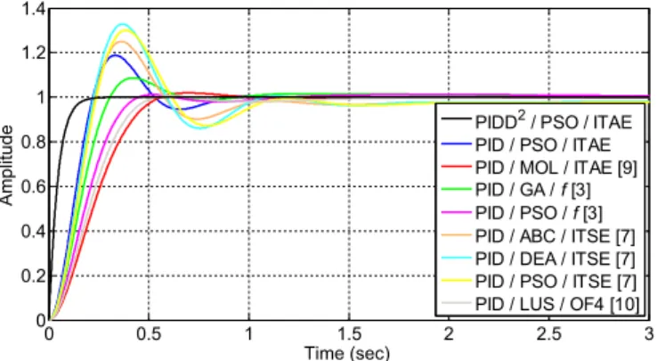
The transient response of the proposed PIDD2controller tuned with PSO is analyzed by comparing the unit-step response with different PID controllers. The PID controllers were designed in recent literature using PSO[3], MOL[9], GA[3], ABC[7], DEA[7], and LUS[10]for the same AVR system.Fig. 9, shows a comparison of the AVR terminal voltage step response of the proposed PIDD2and different PID controllers. Each PID controller is associated with one of the aforementioned tuning algorithms and one objective func-tion. The different objective functions used are the ITAE, integral of time multiplied by squared error (ITSE)[7],ffunction[3], and OF4 function[10], defined by,

0 1 2 3 4 5 6 7 8 -4 -3 -2 -1 0 1 2 3 4 time (sec) e( t) x(t) dx(t)/dt (first order NMF) d x(t)/dt (second order NMF)

Fig. 8.An example illustrating computation offirst and second order derivatives using

NMF.

Table 2

PSO searching parameters.

Parameter Value

Number of iterations (N) 50

Number of trials (T) 10

Swarm size (L) 30

Acceleration constants (c1¼c2) 2

Inertia weight factor (w) [0.9:0.014:0.2]

Table 3

Searching range of parameters.

Parameter Min. value Max. value

Kp 0.0001 3 Ki 0.0001 3 Kd 0.0001 3 Kd2 0.0001 3 vKp 0.6 0.6 vKi 0.6 0.6 vKd 0.6 0.6 vKd2 0.6 0.6

ITAEmin¼ Ztss 0 tjeðtÞjdt; (26) ITSE_min¼ Ztss 0 te2ðtÞdt; (27) fmax¼ 1 1eb_MpþEssþeb_ðtstrÞ; (28) OF4min¼0:8* Ztss 0 e2ðtÞdtþ0:1*tsþ0:1*Mp; (29)

respectively. In Equations(26)e(29),tssis the time at which the response reaches steady state,

b

is a weighting factor, andEssis the steady state error.

FromFig. 9, it can be observed that the proposed PIDD2possess a superior step response behavior compared to other PID con-trollers.Table 4, lists the numerical results of the response com-parison including; controller parameters, the time domain performance indices (Mp,tr,ts, andtp), and the objective function values.

It is clear fromTable 4, that the best response performance indices values, highlighted in bold, are those obtained with the proposed PIDD2controller (Mp¼0,tr¼0.0929,ts¼0.1635, and

tp¼0.32). Therefore, in comparison to all PID controllers, the PIDD2 has the ability to achieve the fastest (minimumtrand ts), most accurate (minimum response oscillation), and most stable (mini-mum overshoot) unit step response.

The proposed PIDD2controller designed by PSO is compared with PID and FOPID controllers designed using CAS algorithm

[12,13,24]. The CAS algorithm is implemented using the parameters listed inTable 5.

Also, the PSO-PIDD2 is compared with PSO-PID [3]and PSO-FOPID controllers [24]. The reciprocal of f defined in Equation

(28)is considered as the objective function to tune the PSO-PID, PSO-FOPID, CAS-PID, and CAS-FOPID with two cases;

b

¼1 and

b

¼1.5. The terminal voltage step responses of the AVR system controlled by PSO-PIDD2, PSO-PID, PSO-FOPID, PID and CAS-FOPID controllers are shown inFig. 10with

b

¼1 and

b

¼1.5.

As can be seen fromFig. 10, the response of the PIDD2is much better than the PID and FOPID controllers tuned with PSO and CAS algorithms in both cases (i.e.

b

¼1 and

b

¼1.5). This can be clearly observed from the time performance indices of all controllers listed in

Table 6.

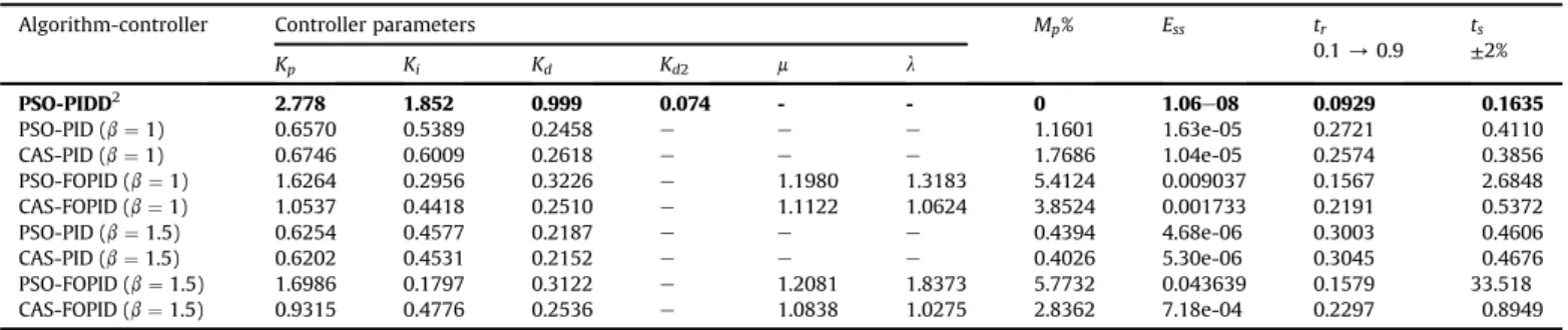
It is observed from Table 6 that the PSO-PIDD2 has the best performance compared to PSO/CAS-PID and PSO/CAS-FOPID con-trollers. The terminal voltage step response of the AVR system controlled by the proposed PIDD2controller has the smallest values ofMp,Ess,tr, andtshighlighted in bold.

The transfer function of the FOPID controllers de_fined by the parameters listed inTable 6, are then implemented with integer orders transfer function using Oustaloup recursive distribution of poles and zeroes approximation[36]. The integer orders transfer function obtained by Oustaloup approximation will have an order equal to 12[24]. This fact adds another preference to the PIDD2 related to implementation complexity. It is worth noting that, the proposed PIDD2 controller can be extended to fractional order PIDD2(PIlDmDm2) where

l

,

m

, and

m

2are non-integer (fractional)

orders of the integral, first and second order derivatives parts respectively. The complexity of this controller is evident due to the increase in the number of control parameters. There are seven different parameters (Kp,Ki,Kd,Kd2,

l

,

m

, and

m

2) that have

to be tuned. The challenge of this work is to develop a realizable FOPIDD2 controller that exhibits a robust performance with fewer parameters, yet achieving the same design requirements. The key point is to look for acceptable and realizable approxi-mations of sl, sm, and sm2 which is recommended for future investigation. 0 0.5 1 1.5 2 2.5 3 0 0.2 0.4 0.6 0.8 1 1.2 1.4 Time (sec) Amplitude

PIDD2 / PSO / ITAE PID / PSO / ITAE PID / MOL / ITAE [9] PID / GA / f [3] PID / PSO / f [3] PID / ABC / ITSE [7] PID / DEA / ITSE [7] PID / PSO / ITSE [7] PID / LUS / OF4 [10]

Fig. 9.Terminal voltage step response of the AVR system with different controllers.

Table 4

Controller parameters and response performance indices of different controllers.

Controller/algorithm/OF Controller parameters Mp% tr

0.1/0.9 ts ±2% tp Obj. value Kp Ki Kd Kd2 PIDD2_{/PSO/ITAE 2.7784 1.8521 0.9997 0.07394 0 0.0929 0.1635 0.3200 0.0018} PID/PSO/ITAE 1.3541 0.9266 0.4378 - 18.805 0.1493 0.8146 0.3276 0.0329 PID/MOL/ITAE[9] 0.5857 0.4189 0.1772 e 1.9539 0.3433 0.5155 0.7036 0.0464 PID/GA/f[3] 0.8861 0.7984 0.3158 e 8.6532 0.2041 0.6058 0.4222 1.1982 PID/PSO/f[3] 0.6568 0.5393 0.2458 e 1.1652 0.2722 0.4111 1.9200 1.4480 PID/ABC/ITSE[7] 1.6524 0.4083 0.3654 e 25.035 0.1559 3.0939 0.3629 0.0177 PID/DEA/ITSE[7] 1.9499 0.4430 0.3427 e 32.830 0.1513 2.6494 0.3636 0.0220 PID/PSO/ITSE[7] 1.7774 0.3827 0.3184 e 30.048 0.1609 3.3994 0.3909 0.0238 PID/LUS/OF4[10] 0.6190 0.4222 0.2058 e 0.5900 0.3123 0.4778 0.6008 0.1677 Table 5

CAS algorithm parameters[24].

Parameter Value

Number of ants (K) 20

Positive constants (a,b) (300, 2/3) Organization factor of anti(ri) 0.04þ0.1rand( ) Initial state of anti(yi(0)) 0.999

jdðd¼1;2;…;5Þ 7:5=ud

Number of iterations 300

rand( ) is a uniformly distributed number in [0, 1]. udis the interval of search of thed-th controller parameter.

7.2. Zero-pole analysis

The overall closed-loop transfer function of the AVR system with the proposed PIDD2controller is of 5th order given by

The zero-pole map of the AVR system with the proposed PIDD2 controller is shown inFig. 11.

It can be observed that the system possess three zero-pole cancellation pairs located at 1,2.5, and10, two real domi-nant poles ats1¼ 24.43 ands1¼ 75.53, and one real zero at z1¼

a

¼ 100. Due to the three zero-pole cancellation, the overall

transfer function in Equation(30)can be approximated to be,

~ G_{AVR_PIDD}2¼ 1845:2 s 100þ1 ðsþ75:53Þ ðsþ24:43Þ (31)

Comparing Equation(31)with the overdamped case of Equation

(7)yields,

a

¼100,r1¼24.43, andr2¼75.53 withr1<r2<

a

. In this

case, the system response possess no overshoot and this can be ensured by substituting the values of

a

,r1, andr2in Equation(16).

The ration of (

a

r2)/(

a

r1) inside the logarithm function is less

than one, thus resulting in a negative time value which indicates no overshoot exists in the system's response.

7.3. Frequency response analysis

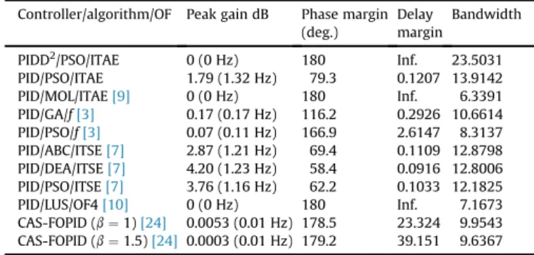
The frequency response of the AVR system with the proposed PIDD2controller is analyzed. The magnitude and phase plots of the AVR with PIDD2controller is shown inFig. 12. The peak gain, phase margin, delay margin and bandwidth obtained from the system's frequency response are depicted inTable 7 and compared with different controllers.

As shown in Table 7, the PIDD2 is the most stable system compared to other controllers. The AVR with PIDD2controller have minimum peak gain 0 dB at 0 Hz, maximum phase margin 180, infinite delay margin (smallest time delay required to make the system unstable), and maximum bandwidth (fastest response). It is worth noting that, a wide bandwidth allows the system to follow arbitrary inputs accurately.

(a) (b) 0 1 2 3 4 5 0 0.2 0.4 0.6 0.8 1 1.2 Time (sec) Am pl itu de 0 0.2 0.4 0.6 0.8 1 0.8 0.9 1 PSO-PIDD2 PSO-PID CAS-PID PSO-FOPID CAS-FOPID 0 1 2 3 4 5 0 0.2 0.4 0.6 0.8 1 1.2 Time (sec) A m pl itu de PSO-PIDD2 PSO-PID CAS-PID PSO-FOPID CAS-FOPID 0 0.2 0.4 0.6 0.8 1 0.8 0.9 1

Fig. 10.Step response of AVR system controlled by PSO-PIDD2_{, PID, CAS-PID,}

PSO-FOPID, and CAS-FOPID (a)b¼1 (b)b¼1.5.

Table 6

Controller parameters and performance indices of PSO-PIDD2_{, PSO-PID, CAS-PID, PSO-FOPID, and CAS-FOPID.}

Algorithm-controller Controller parameters Mp% Ess tr

0.1/0.9 ts ±2% Kp Ki Kd Kd2 m l PSO-PIDD2 _{2.778 1.852 0.999 0.074 - - 0 1.06e08 0.0929 0.1635} PSO-PID (b¼1) 0.6570 0.5389 0.2458 e e e 1.1601 1.63e-05 0.2721 0.4110 CAS-PID (b¼1) 0.6746 0.6009 0.2618 e e e 1.7686 1.04e-05 0.2574 0.3856 PSO-FOPID (b¼1) 1.6264 0.2956 0.3226 e 1.1980 1.3183 5.4124 0.009037 0.1567 2.6848 CAS-FOPID (b¼1) 1.0537 0.4418 0.2510 e 1.1122 1.0624 3.8524 0.001733 0.2191 0.5372 PSO-PID (b¼1.5) 0.6254 0.4577 0.2187 e e e 0.4394 4.68e-06 0.3003 0.4606 CAS-PID (b¼1.5) 0.6202 0.4531 0.2152 e e e 0.4026 5.30e-06 0.3045 0.4676 PSO-FOPID (b¼1.5) 1.6986 0.1797 0.3122 e 1.2081 1.8373 5.7732 0.043639 0.1579 33.518 CAS-FOPID (b¼1.5) 0.9315 0.4776 0.2536 e 1.0838 1.0275 2.8362 7.18e-04 0.2297 0.8949

Fig. 11.Zero-pole map of the AVR system controlled by PIDD2_.

GAVR_PIDD2¼

18:4855ðsþ100Þðsþ10:02Þðsþ2:501Þðsþ0:9994Þ

7.4. Robustness analysis

Robustness analysis is used to evaluate the controller ability to tolerate uncertainties exists in some system parameters. In this subsection, the PIDD2controller is tested against uncertainties of AVR system parameters. The uncertainties of the AVR model are specified in terms of variations in the amplifier, exciter generator, and sensor time constants (Ta,Te,Tg, andTsrespectively) above and below their nominal values. The variation range of the time con-stants is chosen to be±50% of their nominal values with a 25% step size.Figs. 13_e16show step responses of the PIDD2_{controlled AVR}

system with Ta, Te, Tg, and Ts time constants variations about nominal responses respectively.

It can be realized from Figs. 13e16, that the deviations of response curves (±50% and±25%) from the nominal response for the selected time constant parameters are within a small range. This can ensures the ability of the PIDD2to maintain stability and to

perform properly despite such large variations. Tables 8 and 9

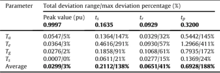
present a summary of the PIDD2 robustness analysis results and list the total deviation ranges and maximum deviation percentage of the system respectively.

From Table 9, the average deviation of maximum overshoot, settling time, rise time and peak time are 3%, 138%, 41% and 188% respectively. The ranges of total deviation are acceptable and are within limit. Therefore, it can be concluded that the AVR system with the proposed PIDD2controller is robust and can still perform acceptable control behavior.

7.5. Digital implementation

The realization of the proposed PIDD2controller and its discrete implementation is tested in SIMULINK®and compared with PID/ MOL[9]and PID/GA[3]discrete controllers. The general Simulink model of the AVR control system is shown inFig. 17.

Table 7

Bode analysis of different AVR controllers.

Controller/algorithm/OF Peak gain dB Phase margin (deg.)

Delay margin

Bandwidth PIDD2_{/PSO/ITAE 0 (0 Hz) 180 Inf. 23.5031}

PID/PSO/ITAE 1.79 (1.32 Hz) 79.3 0.1207 13.9142 PID/MOL/ITAE[9] 0 (0 Hz) 180 Inf. 6.3391 PID/GA/f[3] 0.17 (0.17 Hz) 116.2 0.2926 10.6614 PID/PSO/f[3] 0.07 (0.11 Hz) 166.9 2.6147 8.3137 PID/ABC/ITSE[7] 2.87 (1.21 Hz) 69.4 0.1109 12.8798 PID/DEA/ITSE[7] 4.20 (1.23 Hz) 58.4 0.0916 12.8006 PID/PSO/ITSE[7] 3.76 (1.16 Hz) 62.2 0.1033 12.1825 PID/LUS/OF4[10] 0 (0 Hz) 180 Inf. 7.1673 CAS-FOPID (b¼1)[24] 0.0053 (0.01 Hz) 178.5 23.324 9.9543 CAS-FOPID (b¼1.5)[24] 0.0003 (0.01 Hz) 179.2 39.151 9.6367

Fig. 13.Step response curves ranging from50% toþ50% forTa.

Fig. 14.Step response curves ranging from50% toþ50% forTe.

Fig. 15.Step response curves ranging from50% toþ50% forTg.

Fig. 16.Step response curves ranging from50% toþ50% forTs.

-30 -20 -10 0 Magnitude (dB) 10 10 10 10 10 -90 -45 0 Phase (deg) Bode Diagram Frequency (rad/s)

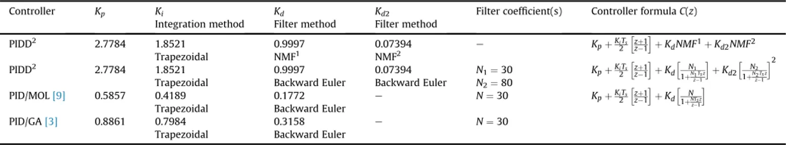
The controller subsystem, shown inFig. 17, is implemented by a discrete PIDD2 or PID controller having specifications defined in

Table 10.

The sampling time (Ts) is chosen according to the rule of thumb suggested by Astrom and Wittenmark such that the product ofTs and the gain crossover frequency (

uc

in radians per second) of the loop gainðC_PIDD2GaGeGgHsÞ, is between 0.15 and 0.5[32]. The gain crossover frequency of the AVR control system loop gain is

uc

¼18.2 radian per second. Thus, an appropriate sampling time is between

0.008 and 0.0275 (Tsis set to 0.01). The response of the PIDD2, PID/MOL[9], and PID/GA[3]controllers are tested at steady state by subjecting a disturbance load signals of values equal to þ10% and10% of the set point at times 3 and 5 s respectively.Figs. 18 and 19show the set point responses due to the unit step input at

t¼0 and responses due to load disturbances att¼3 and 5 s along with the controller outputs.

Compared to PID/MOL[9]and PID/GA[3]controllers, the pro-posed PIDD2with NMF (PIDD2/NMF) posses an improved set point and load disturbance responses as shown inFig. 18. The responses of PIDD2withfilteredfirst and second derivative actions (PIDD2/

N1N2) are faster than those of PID/MOL[9] and PID/GA[3]

con-trollers, however, it has the highest maximum overshoots values. In AVR control system, the controller actions are carried out as a response to load disturbance (regulating system) not to set point changes (tracking system). Therefore, inFig. 19, only the responses to load disturbances are shown. It can be observed that the range of the controller output signals for the PIDD2/NMF, PID/MOL[9], and PID/GA [3] controllers are ±3.8, ±0.7, and ±0.44 respectively. However, for PIDD2/N1N2 controller, the range of the controller

output signal exceeds±4.

Controllers are designed to work with nonlinear behavior of process actuators. The actuator device, such as the amplifier in the AVR system, has a limited range of input and output operation. Such limitations appear at the input of the actuator and are modeled with a non-linear element having saturation characteristics. Moreover, when abrupt change occurs in the system output due to a load disturbance, the controller output will exhibit a large spike values similar to those of the PIDD2/NMF shown inFig. 19. These spikes are mainly due to thefirst and second derivative actions and could be detrimental to the operation of the actuator unit. To avoid subjecting the actuator unit to such large controller output values, a constrained action defined by the maximum and minimum output range limits of the actuator. However, in this case the integral action will produce an inaccurate and highly excessive value causing oscillation and slowing down the transient response. This behavior is called the integrator windup problem. This can be solved by several anti-windup algorithms such as the configuration sug-gested by Wilkie et al.[37].

Table 8

Robustness analysis results of the AVR system with the proposed PIDD2_controller.

Parameter Rate of change (%) Peak value (pu) ts tr tp

Ta 50% 0.9994 0.3352 0.1226 0.7836 25% 0.9967 0.2674 0.0897 0.4794 þ25% 1.0243 0.2964 0.1005 0.2394 þ50% 1.0514 0.4038 0.1084 0.2476 Te 50% 0.9985 0.5242 0.0395 1.6345 25% 0.9972 0.2615 0.0685 1.0805 þ25% 1.0173 0.1770 0.1139 0.3379 þ50% 1.0336 0.6386 0.1325 0.3698 Tg 50% 0.9910 0.3119 0.0362 0.0717 25% 0.9940 0.1261 0.0648 0.8705 þ25% 1.0096 0.1952 0.1189 0.4176 þ50% 1.0186 0.2243 0.1430 0.4687 Ts 50% 0.9997 0.1896 0.1067 0.3801 25% 0.9997 0.1774 0.1000 0.3532 þ25% 0.9996 0.1471 0.0857 0.2703 þ50% 1.0003 0.1285 0.0790 0.2441 Table 9

Total deviation ranges and maximum deviation percentage of the system. Parameter Total deviation range/max deviation percentage (%)

Peak value (pu)

0.9997 ts 0.1635 tr 0.0929 tp 0.3200 Ta 0.0547/5% 0.1364/147% 0.0329/32% 0.5442/145% Te 0.0364/3% 0.4616/291% 0.0930/57% 1.2966/411% Tg 0.0276/2% 0.1858/91% 0.1068/61% 0.7935/172% Ts 0.0007/0% 0.0611/21% 0.0277/15% 0.1369/24% Average 0.0299/3% 0.2112/138% 0.0651/41% 0.6928/188%

The results as summarized inTable 11indicate that the response of the proposed PIDD2/NMF controller outperforms the responses of the PIDD2/N1N2, PID/MOL [9], and PID/GA [3] in terms of

maximum overshoot, rise time, and settling time. The best response performance indices values of the proposed PIDD2/NMF controller are highlighted in bold.

8. Conclusion

In this paper, a novel PID plus second order derivative controller (PIDD2) is proposed to control AVR system. The proposed PIDD2 consists of four control terms; proportional, integral, derivative, and second derivative. The PSO algorithm with the integral of time multiplied by absolute error (ITAE) performance criterion is used to tune the four gains of the PIDD2controller. The performance of the AVR with PIDD2is compared with several PID controllers tuned by recently proposed approaches, such as MOL, GA, ABC, DEA, and LUS. In addition, the proposed PIDD2 is compared with the FOPID controller designed by using CAS algorithm. Simulation results show a superior response performance of the proposed PIDD2. Moreover, the frequency response, zero-pole, and robustness analysis performed on the PIDD2controller showed more robust stability and better performance characteristics than the PID and FOPID controllers.

References

[1] P. Kundur, N.J. Balu, M.G. Lauby, Power System Stability and Control, vol. 7, McGraw-Hill, New York, 1994.

[2] A. Kiam Heong, G. Chong, L. Yun, PID control system analysis, design, and technology, IEEE Trans. Control Syst. Technol. 13 (4) (2005) 559e576. [3] G. Zwe-Lee, A particle swarm optimization approach for optimum design of

PID controller in AVR system, IEEE Trans. Energy Convers. 19 (2) (2004) 384e391.

[4] P. Wang, D.P. Kwok, Optimal design of PID process controllers based on ge-netic algorithms, Control Eng. Pract. 2 (4) (1994) 641e648.

[5] V. Mukherjee, S.P. Ghoshal, Intelligent particle swarm optimized fuzzy PID controller for AVR system, Electr. Power Syst. Res. 77 (12) (2007) 1689e1698. [6] M. Kashki, Y. Abdel-Magid, M. Abido, A reinforcement learning automata optimization approach for optimum tuning of PID controller in AVR system, in: D.-S. Huang, et al. (Eds.), Advanced Intelligent Computing Theories and Applications. With Aspects of Artificial Intelligence, Springer Berlin, Heidel-berg, 2008, pp. 684e692.

[7] H. Gozde, M.C. Taplamacioglu, Comparative performance analysis of artificial bee colony algorithm for automatic voltage regulator (AVR) system, J. Franklin Inst. 348 (8) (2011) 1927e1946.

[8] G. Reynoso-Meza, et al., Controller tuning using evolutionary multi-objective optimisation: current trends and applications, Control Eng. Pract. 28 (0) (2014) 58e73.

[9] S. Panda, B.K. Sahu, P.K. Mohanty, Design and performance analysis of PID controller for an automatic voltage regulator system using simplified particle swarm optimization, J. Franklin Inst. 349 (8) (2012) 2609e2625.

[10] P.K. Mohanty, B.K. Sahu, S. Panda, Tuning and assessment of proportio-naleintegralederivative controller for an automatic voltage regulator system employing local unimodal sampling algorithm, Electr. Power Compon. Syst. 42 (9) (2014) 959e969.

[11] H. Zhu, et al., CAS algorithm-based optimum design of PID controller in AVR system, Chaos Solitons Fractals 42 (2) (2009) 792e800.

[12] L. Li, et al., An optimization method inspired by“chaotic”ant behavior, Int. J. Bifurcation Chaos 16 (08) (2006) 2351e2364.

[13] L. Li, et al., Parameters identification of chaotic systems via chaotic ant swarm, Chaos Solitons Fractals 28 (5) (2006) 1204e1211.

[14] L. Li, et al., Chaoseorder transition in foraging behavior of ants, Proc. Natl. Acad. Sci. 111 (23) (2014) 8392e8397.

[15] L. Li, Y. Yang, H. Peng, Fuzzy system identification via chaotic ant swarm, Chaos Solitons Fractals 41 (1) (2009) 401e409.

[16] S. Das, et al., A novel fractional order fuzzy PID controller and its optimal time domain tuning based on integral performance indices, Eng. Appl. Artif. Intell. 25 (2) (2012) 430e442. 0 1 2 3 4 5 6 7 8 0.8 0.9 1 1.1 1.2 1.3 1.4 Time (sec) Te rm in al V ol ta ge ( p.u .) PIDD2_/NMF PIDD2/N₁N₂ PID/MOL PID/GA 5 5.5 6 0.9 1

Fig. 18.Set-point and disturbance responses the AVR control system.

3 3.5 4 4.5 5 5.5 6 -4 -3 -2 -1 0 1 2 3 4 time (sec) Controller Output PIDD2/NMF PIDD2/N₁N₂ PID/MOL PID/GA

Fig. 19.Controller output.

Table 11

Performance comparison.

Controller Set-point response Load-disturbance response

Mp% tr ts Mp% tr ts PIDD2_{/NMF 10 0.08 0.16 9.3 0.09 0.18} PIDD2_/N 1N2 39 0.10 0.49 38 0.11 0.50 PID/MOL[9] 10 0.43 1.27 10 0.45 0.28 PID/GA[3] 29 0.28 1.36 28 0.30 1.36 Table 10

Controller subsystem specifications. Controller Kp Ki Integration method Kd Filter method Kd2 Filter method

Filter coefficient(s) Controller formulaC(z)

PIDD2 _{2.7784 1.8521} Trapezoidal 0.9997 NMF1 0.07394 NMF2 e KpþKiTs 2 h zþ1 z1 i þKdNMF1_þKd 2NMF2 PIDD2 _{2.7784 1.8521} Trapezoidal 0.9997 Backward Euler 0.07394 Backward Euler N1¼30 N2¼80 KpþKiTs 2 h zþ1 z1 i þKdh N1 1þN1Ts z z1 i þKd2 h N2 1þN2Ts z z1 i2 PID/MOL[9] 0.5857 0.4189 Trapezoidal 0.1772 Backward Euler e N¼30 KpþKiTs 2 h zþ1 z1 i þKdh N 1þNTs z z1 i PID/GA[3] 0.8861 0.7984 Trapezoidal 0.3158 Backward Euler e N¼30

[17] A. Rajasekhar, R. Kumar Jatoth, A. Abraham, Design of intelligent PID/ PIlDmspeed controller for chopper fed DC motor drive using opposition based artificial bee colony algorithm, Eng. Appl. Artif. Intell. 29 (0) (2014) 13e32.

[18] R. El-Khazali, Fractional-order controller design, Comput. Math. Appl. 66 (5) (2013) 639e646.

[19] I. Podlubny, Fractional-order systems and PI/sup/spl lambda//D/sup/spl mu//-controllers, IEEE Trans. Auto. Control 44 (1) (1999) 208e214.

[20] A. Biswas, et al., Design of fractional-order PIlDmcontrollers with an improved differential evolution, Eng. Appl. Artif. Intell. 22 (2) (2009) 343e350. [21] N. Aguila-Camacho, M.A. Duarte-Mermoud, Fractional adaptive control for an

automatic voltage regulator, ISA Trans. 52 (6) (2013) 807e815.

[22] M. Zamani, et al., Design of a fractional order PID controller for an AVR using particle swarm optimization, Control Eng. Pract. 17 (12) (2009) 1380e1387. [23] I. Pan, S. Das, Chaotic multi-objective optimization based design of fractional

order PIlDmcontroller in AVR system, Int. J. Electr. Power Energy Syst. 43 (1) (2012) 393e407.

[24] Y. Tang, et al., Optimum design of fractional order PIlDmcontroller for AVR system using chaotic ant swarm, Expert Syst. Appl. 39 (8) (2012) 6887e6896.

[25] F. Merrikh-Bayat, S.-N. Mirebrahimi, M.-R. Khalili, Discrete-time Fractional-order PID Controller: Definition, Tuning, Digital Realization and Experimental Results. arXiv preprint arXiv:1405.0144, 2014.

[26] I. Pan, S. Das, Frequency domain design of fractional order PID controller for AVR system using chaotic multi-objective optimization, Int. J. Electr. Power Energy Syst. 51 (0) (2013) 106e118.

[27] K. Ogata, Modern Control Engineering, Prentice Hall, 2010.

[28] J. Kennedy, R. Eberhart, Particle swarm optimization, in: IEEE International Conference on Neural Networks, 1995.

[29] A. Ertas, Optimization offiber-reinforced laminates for a maximum fatigue life by using the particle swarm optimization. Part II, Mech. Compos. Mater. 49 (1) (2013) 107e116.

[30] S. Yuhui, R. Eberhart, A modified particle swarm optimizer, in: The 1998 IEEE International Conference on Evolutionary Computation Proceedings, 1998. IEEE World Congress on Computational Intelligence, 1998.

[31] J. Kennedy, The particle swarm: social adaptation of knowledge, in: IEEE In-ternational Conference on Evolutionary Computation, 1997.

[32] K.J. Åstr€om, B. Wittenmark, Computer-controlled Systems: Theory and Design, Courier Dover Publications, 2011.

[33] L. Yun, A. Kiam Heong, G.C.Y. Chong, PID control system analysis and design, IEEE Control Syst. 26 (1) (2006) 32e41.

[34] R.A. Krohling, J.P. Rey, Design of optimal disturbance rejection PID controllers using genetic algorithms, IEEE Trans. Evol. Comput. 5 (1) (2001) 78e82. [35] Y. Del Valle, et al., Particle swarm optimization: basic concepts, variants and

ap-plications in power systems, IEEE Trans. Evol. Comput. 12 (2) (2008) 171e195. [36] A. Oustaloup, et al., Frequency-band complex noninteger differentiator:

characterization and synthesis, IEEE Trans. Circuits Syst. I Fundam. Theory Appl. 47 (1) (2000) 25e39.

[37] J. Wilkie, M. Johnson, R. Katebi, Control Engineering: an Introductory Course, Palgrave, 2003.