Modeling Nested Copulas with GLMM Marginals for Longitudinal Data

(1)

Modeling Nested Copulas with GLMM Marginals for Longitudinal Data Roba Bairakdar A Thesis in The Department of

Mathematics and Statistics

Presented in Partial Fulfillment of the Requirements for the Degree of Master of Science (Mathematics) at

Concordia University Montreal, Quebec, Canada

December 2017 © Roba Bairakdar, 2017

(2)

CONCORDIA UNIVERSITY

School of Graduate Studies

This is to certify that the thesis prepared By: Roba Bairakdar

Entitled: Modeling Nested Copulas with GLMM Marginals for Longitudinal Data and submitted in partial fulfillment of the requirements for the degree of

Master of Science (Mathematics)

complies with the regulations of the University and meets the accepted standards with respect to originality and quality.

Signed by the final Examining Committee:

Examiner Dr. F. Godin Examiner Dr. L. Kakinami Co-supervisor Dr. F. Ducharme Supervisor Dr. M. Mailhot Approved by

Chair of Department or Graduate Program Director

Dean of Faculty

(3)

Abstract

Modeling Nested Copulas with GLMM Marginals for Longitudinal Data

A flexible approach for modeling longitudinal data is proposed. The model consists of nested bivariate copulas with Generalized Linear Mixed Models (GLMM) marginals, which are tested and validated by means of likelihood ratio tests and compared via theirAICc andBIC values. The copulas are joined together through a vine structure. Rank-based methods are used for the estimation of the copula parameters, and appropriate model validation methods are used such as the Cram´er Von Mises goodness-of-fit test. This model allows flexibility in the choice of the marginal distributions, provided by the family of the GLMM. Additionally, a wide vari-ety of copula families can be fitted to the tree structure, allowing different nested dependence structures. This methodology is tested by an application on real data in a biostatistics study.

(4)

Acknowledgments

This thesis reached its final form by the kind support and encouragement of many individuals, to whom I would be eternally grateful. I would like to start by thanking Allah for providing me with the strength and motivation that I required in this journey.

I am extremely thankful to my supervisor Professor M´elina Mailhot for her invaluable direction, trust and encouragement. Her optimistic nature is contagious, and I always look forward to our meetings to get the positive energy boost needed for this research. She has gone out of her way several times to provide me with the best opportunities for this thesis and for my future, and I am forever indebted to her.

I would also like to thank Dr. Francine Ducharme who provided me with the opportunity to col-laborate with the research center at Centre Hospitalier Universitaire Sainte-Justine. Her insightful thoughts and massive amount of medical knowledge were extremely useful in this research. Further-more, I would like to thank Professor Frédéric Godin and Professor Lisa Kakinami for reviewing my thesis and for their comments that helped in improving it. I am thankful to Professor Johanna Neˇslehová for allowing me to attend her class to learn from her immense knowledge and for her advice on numerous occasions. I would also like to thank the mathematics and statistics department at Concordia and my supervisor for providing me with financial support during my Masters.

My gratitude goes to all my professors throughout my academic journey that spanned across two continents, specifically professors Zeinab Amin, Aliaa Bassiouny, Frédéric Godin, Ali Hadi, Mélina Mailhot, Étienne Marceau, Magdi Moustafa, Johanna Neˇslehová and Lea Popovic, presented alpha-betically by their surnames.

A special thank you note goes to my friends, from all over the world, for their moral support, and making me feel home away from home. I would also like to mention my students who brought me here in the first place and always remind me of my sense of purpose. Sincere appreciation goes to my family, specifically my mother, grandmother, aunt and brother. It is painful to be thousands of kilometers away from them, but they always find a way to make that distance emotionally shorter. Finally, I am grateful for my father’s support; your memory will always be with me.

To my backbone; my mother, grandmother and aunt: Lama, Samira and Rama.

(5)

List of Figures

1.1 Illustration of OLS regression. The straight line minimizes the squared differences between the observed response and the predicted values, indicated by the blue vertical lines. . . 3 2.1 Illustration of the rectangle inequality for a bivariate distribution . . . 22 2.2 Perspective plots of the cdf of the Countermonotonicity copula, Independence

copula and Comonotonicity copula. . . 30 2.3 Perspective plots of the densities of the bivariate Gauss copula withρ= 0.9238795

and bivariatet-copula with ρ= 0.9238795 andν = 2. . . 32 2.4 Top: One thousand simulated points from the Gaussian copula withρ= 0.9238795

and bivariate t-copula with ρ = 0.9238795 and ν = 2. Bottom: Realizations of X1 andX2 by assuming standard normal marginals for the copulas presented on

the top row. . . 32 2.5 Perspective plots of the densities of the bivariate Clayton copula, bivariate Frank

copula, and bivariate Gumbel copula. The dependence parameter for each copula isθ= 6,14.1385 and 4, respectively. . . 35 2.6 Top: One thousand simulated points from the Clayton, Frank and Gumbel

cop-ulas with dependence parameter for each copula is θ = 6,14.1385 and 4, re-spectively. Bottom: Realizations of X1 and X2 by assuming standard normal

marginals for the copulas presented on the top row.. . . 35 2.7 A basic vine structure. . . 38 2.8 The attainable correlations ρmin_p and ρmax_p for X1 ∼ LogNormal(0,1) and X2 ∼

(8)

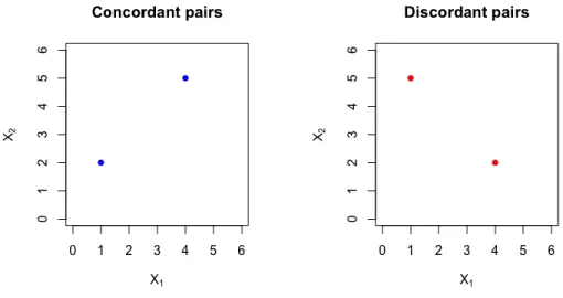
2.9 Relationship between Spearman’s rhoρS, Kendall’s Tauτ and Pearson’s correla-tion coefficient ρp for Gauss Copula. . . 48 2.10 On the left, a pair of concordant points, and on the right, a pair of discordant

points. . . 49 4.1 The tree structure used for modeling longitudinal data with 4 responses. . . 62 5.1 The mean of Y(1) over time split by treatment type and study. . . 74 5.2 Q-Q plot of the residuals of the model with the parameters specified in 5.7. . . . 76 5.3 The mean of Y(2) over time split by treatment type and study. . . 77 5.4 95% confidence intervals of the estimates of random effects for the intercept in

(9)

List of Tables

1.1 Characteristics of some common exponential family members as shown by Mc-Cullagh (1984). . . 10 2.1 Summary of the generators φ(t), where t ∈ [0,1], the possible values for the

dependence parameterθ, and the limiting cases for some bivariate Archimedean copulas. . . 36 2.2 Spearman’s rho ρS and Kendall’s tau τ for the copula families discussed in 2.2.1. 52 5.1 p-value of the LRTs on the GLM models for the amount of vitamin D at each

visit. The LRTs compare the model with all predictors and the parsimonious model obtained from the stepwise variable selection. . . 68 5.2 Patients Characteristics at each visit. Numerical variables are associated with

the mean and the 95% confidence interval. . . 69 5.3 AICc of the optimal GLM models for the amount of vitamin D at each visit,

obtained by stepwise variable selection.. . . 70 5.4 Transformed parameter estimates and their 95% confidence intervals for the Gamma

GLM models for the amount of vitamin D at each visit. . . 71 5.5 Patients Characteristics for the longitudinal study. Numerical variables are

asso-ciated with the mean and the 95% confidence interval. . . 72 5.7 Parameter estimates and their 95% confidence intervals for the OLS model for

the change in the amount of vitamin D between visits. . . 76 5.8 Parameters estimates, transformed parameters estimates and their 95%

confi-dence intervals for the GLM model for the number of asthma attacks that require the use of OCS between visits. . . 79

(10)

5.9 Estimates for dependence measures between ˆ(1)_ij and ˆ(2)_ij . . . 81 5.10 Estimates of copula parameters, p-values of goodness of fit test, AICc and BIC

(11)

Introduction

Modeling the dependence structure for multivariate longitudinal data is an important challenge in all fields. In the literature, it is usually assumed that the data, or a transformation of the data, is generated from a multivariate normal distribution, with a variance-covariance matrix that explains the dependence between the multiple response variables, and the serial dependence. However, we often come across data that are not normally distributed, and hence, a generalized methodology is needed to fit all distributions. Furthermore, assuming a common distribution for all the responses might not be appropriate. Therefore, in this thesis, we propose a parametric approach for a nested copula model for fitting multiple responses of longitudinal data, where each response is initially modeled by a generalized linear mixed model. This allows for the possibility of using a variety of continuous and discrete distributions. Under this approach, the marginal distributions take into account the dependence between each response and its covariates, over time, while the copula holds the general structure for the dependence between each response. Instead of measuring the linear correlation, we examine a more general and appropriate concept of dependence. The estimates for the marginal distributions are obtained by fitting each re-sponse to multiple distributions that fit its characteristics, where afterwards variable and model selection criteria are performed to choose the best fit model. Additionally, the estimates for the dependence parameters of the copula is obtained by maximizing the pseudo log-likelihood by using rank-based methods. An inadequate choice for the dependence parameter and copula may result in unexpected deviations in the response variable, especially when one is provided with a small data set. Therefore, goodness of fit tests are performed to ensure the accuracy of the model. The model can be used for predictive modeling and conditional predictive modeling, where the choice of the conditioning response variable is arbitrary and is chosen based on the context of the data.

(12)

Our methodology is applied to real data in biostatistics, provided by the research center of Centre Hospitalier Universitaire Sainte-Justine, Montreal, QC. This data set has been the mo-tivation behind this research.

This thesis is structured as follows. In Chapter 1, we discuss different regression models to fit data with only one outcome variable. The assumptions and properties of each model are explained in details. Chapter 2 introduces multivariate distributions and their link with cop-ulas. Several properties of different copula families are explored. We also explain measures of dependence and how to use copulas for predictions. In Chapter3, we explain different criteria to choose the model and variables that provide the best fit for any data. A small number of observations can be restrictive in modeling, and special criteria are mentioned to overcome this problem. We propose a model that is appropriate for modeling multivariate longitudinal data in Chapter 4. This model provides flexibility in modeling responses from various distributions, with different pairwise dependence structure. Additionally, in Chapter5, we provide a real life application in biostatistics for the suggested model and we illustrate the procedure for predictive modeling simulations.

(13)

Chapter 1

Univariate Models

Linear regression is used to model the relationship between a response variable, also called the dependent variable, outcome variable, predicted variable or regressand and denoted by y, and a set of predictors, also called the independent variables, explanatory variables, covariates or regressors and denoted by x1, x2, . . . , xp, by assuming a linear relationship between them. If there is only one predictor x1, this is referred to as Simple Linear Regression, however if there

are two or more predictors, it is referred to as Multiple Linear Regression (MLR). The goal of linear regression is to identify the strength of the linear relationship between the response variable and each predictor, identify the predictors that have no effect on the response variable and to predict values for the response variable using any values for the predictors. Given a real data set, we do not know the parameters of the model, but we can explain the relationship between the response variable and the predictors by estimating the model parameters and using them to identify the conditional expectation of the response variable given the predictors. There are several methods to fit linear models, some of which will be explained in this thesis where the availability of more than one predictor (i.e. MLR) is assumed. The discussed methods are Ordinary Least Squares (OLS), Generalized Linear Models (GLM) and Generalized Linear Mixed Models (GLMM). There are also non-linear regression models that assume that the relationship between the dependent variable and the independent variables is non-linear in terms of the regression parameters, but they will not be explored further in this thesis due to their complexity. Linear models are more commonly used as they can be easily modeled and explained.

(14)

1.1 Ordinary Least Squares

The earliest method for estimating the parameters of a linear model is the Ordinary Least Squares (OLS) method, which was first used by Gauss and Legendre as explained in Stigler

(1981) who applied the model to astronomical data sets. The goal of OLS is to find the linear model that minimizes the square of the prediction error.

1.1.1 The Model

Consider a data set that containsnobservations. Each observationiconsists of a scalar response variableyi and a set ofp predictors xij for j= 1, . . . , p. The relationship between the response variable and the predictors for observation i are assumed to be linear in parameters, but not necessarily linear in predictors. This means that, for example, the variables xij can be to any power, but the parameters of the model have to maintain the linearity assumption. The general form for OLS is

yi =β0+β1xi1+. . .+βpxip+i,

whereβ0 is called the model intercept,β1, . . . , βp are the regression coefficients andi is the ran-dom error, which is the difference between the actual observed value of the response variable, and the predicted value from using the above model. Each regression coefficient represents an additive change in the expected value of y resulting from a one unit increase in the predictor associated with that regression coefficient. It is assumed that∼N(0, σ2), all i’s are indepen-dent and that the predictors are nearly linearly indepenindepen-dent (no strong multi-collinearity). All those assumptions will be discussed later in Section1.1.3. The above model can be rewritten in matrix notation as follows:

n×1 z}|{ Y = n×1 z }| { X |{z} n×(p+1) β |{z} (p+1)×1 + n×1 z}|{ ,

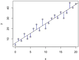
where all entries in the first column of X are equal to 1. The goal of OLS is to find estimates for the regression coefficients ˆβ0,βˆ1, . . . ,βˆp that minimize the squared differences between the observed response variable yi, and the predicted values ˆyi = ˆβ0 + ˆβ1xi1 +. . .+ ˆβpxip. The difference yi−yˆi is called the regression residuals, and it is represented by the blue lines in Figure1.1.

(15)

Figure 1.1: Illustration of OLS regression. The straight line minimizes the squared differences between the observed response and the predicted values, indicated by the blue vertical lines.

1.1.2 Estimation of Model Parameters

The regression coefficients of the OLS model can be obtained by solving ˆ β0,βˆ1, . . . ,βˆp = arg min (β0,β1,...,βp) n X i=1 (yi−yˆi)2, or its equivalent in matrix notation

ˆ

β= arg min β∈R(p+1)

kY −Xβk2. (1.1.1)

Letf(β) be the objective function in the optimization of Eq. 1.1.1, then f(β) =kY −Xβk2 =YTY −2βTXTY +βTXTXβ, and ∂f(β) ∂β =−2X T_Y _{+ 2X}T_X_β_{= 0.} This leads to the following regression coefficient estimates

ˆ

β= XTX−1XTY, (1.1.2)

(16)

1.1.3 Assumptions

It is important to validate the required assumptions for fitting OLS regression to the data, otherwise, we can have incorrect and misleading results. Those assumptions are explained in details in Allen(1997) and are summarized in the following points,

Assumption 1. The linear regression model is linear in parameters.

The relationship between the response variableY and the predictorsX’s is linear in parameters β and not necessarily linear inX’s. Therefore, Eq. I and Eq. II are acceptable, but Eq. III is not acceptable;

yi =β0+β1xi1+. . .+βpxip+i, (I) yi =β0+β1x2i1+. . .+βpxp_ip+i, (II) yi =β0+β12xi1+. . .+βppxip+i. (III)

Assumption 2. The observations in the data set are independent and sampled randomly such that the number of observationsy1, . . . , yn is bigger than the number of parameters β.

Independence of the observations is one of the important assumptions because it assures that we have a model with only fixed effects, and no random effects. Random effects can occur when the observations can be grouped in different categories, such that each category varies uniquely from the mean of the population. Section1.3further explains random effects and the changes that occur in the modeling as a result of their presence. In addition, if the number of observationsnis equal to the number of parametersp, then we have equal number of equations as unknowns, which can be solved algebraically without the need for OLS. If n < p, a unique solution is impossible to find algebraically or by using OLS.

Assumption 3. Multi-collinearity should be minimized.

There should be almost no linear relationship between the predictors. If there is a strong linear relationship (Pearson correlation coefficient ρp close to ±1) between the predictors, we should drop some of them such that the chosen model has almost uncorrelated predictors.

Assumption 4. The predictors are non-random.

The predictorsxi1, . . . , xipare assumed to have fixed values such that variation in the predictors causes variation in the outcomeyi. However, changes in the outcome should not imply changes

(17)

in the predictors. In other words, if we are modeling the amount of auto insurance losses, then it is assumed that the amount of the loss depends on the car type, but the car type does not depend on the amount of the loss.

Assumption 5. ∼N(0, σ2).

The error terms should be independent and identically distributed (IID) with mean 0 and con-stant varianceσ2, and given the previous assumption, this makes the response variable random as well. In addition, there should be no relationship between the predictors and .

If we consider the case where the response variable Y is Normally distributed such that Y ∼ N(Xβ, σ2In), then the maximum likelihood estimates ofβresults in the same estimates obtained by OLS.

Proof. To obtain the estimates of the parameters β and σ2, we use the maximum likelihood estimation method. The density function is

φ Y;Xβ, σ2In = (2π)−n/2|σ−2_I n|1/2exp −1 2(Y −Xβ) T _σ−2_I n(Y −Xβ) ,

and its log-likelihood function is l β, σ2;Y, X =−n 2log(2π) + 1 2log|σ −2_I n| − 1 2(Y −Xβ) T_σ−2_I n(Y −Xβ) =−n 2log(2π) + n 2logσ −2₋1 2σ −2_(Y ₋_X_β₎T (Y −Xβ). Therefore, the maximum likelihood estimator is obtained by optimizing

ˆ β,σˆ2 = arg min (β,σ2₎_∈ R(p+1)×R+ −l β, σ2;Y, X.

The partial derivatives of the objective function with respect to each parameter is equated to 0 as follows: ∂ −l β, σ2;Y, X ∂σ2 = n 2σ2 − 1 2σ4 (Y −Xβ) T _(Y ₋_X_β_{) = 0} σ2= 1 n(Y −Xβ) T_(Y ₋_X_β₎_, and, ∂−l β, σ2;Y, X ∂β, = 1 2σ −2∂ h (Y −Xβ)T (Y −Xβ) i ∂β

(18)

= 1 2σ −2∂ YTY −2βTXTY +βTXTXβ) ∂β = 1 2σ −2 _−2XT_Y _{+ 2X}T_X_β = 0 ˆ β= XTX−1 XTY.

Therefore, when the outcome variable is normally distributed, the estimates of the regression coefficients are identical to those obtained by OLS, as shown in Eq. 1.1.2, provided thatXTX is invertible.

1.1.4 Goodness of Fit Measures

The closer the predicted values obtained from the fitted model ˆyare to the observed values from the data y, the better the fit of the model. There are several measures that can be used to asses the accuracy of the fitted model and to compare different models together. They will be discussed in Chapter3.1.

1.2 Generalized Linear Models

Even though OLS provides a relatively simple method to fit data sets, it has some restrictions that may prevent us from applying it. As explained byMcCullagh (1984), Generalized Linear Models (GLMs) are an extension of linear models where the mean of the response variable is linearly related to the predictors via an arbitrary link function and the variance of the response variable depends on the mean. This means that a function of E(Y) is linearly related to the

predictors, rather than the response variable itself being linearly related to the predictors. GLMs also allow us to drop the normality assumption of the error terms under the OLS (i.e. i does not have to be normally distributed with zero-mean and constant variance σ2). In addition, by using GLM, we have the flexibility to model data where the response variable is bounded or discrete. GLMs assumes independence of the observations, and hence there are only fixed effects in the model. Section1.3will discuss the modeling performed when there is dependence between the observations. Further assumptions of GLM are discussed in Section1.2.5.

(19)

1.2.1 The Model

Consider a model with response vector Y = (y1, . . . , yn), and p predictors arranged in a n×p matrixX wherenrepresents the number of observations. The responsesy1, . . . , ynare assumed to be independent and generated from the same exponential family, which is discussed in details in Section 1.2.2. The mean of the response vector Y is assumed to be linearly related to the predictors via an arbitrary link function g(·) as follows:

g(E[Y]) =g(µ) =Xβ=η,

whereβ is the vector of regression coefficients, which is usually estimated using the maximum likelihood method. η is called the linear predictor and its components can be defined by

ηi = p X

j=1

xijβj =XiTβ.

The true mean of the response variable can be calculated by taking the inverse of the link function (i.e. E[Y] =g−1(Xβ) =g−1(η)) and the variance V ar(Y) is a function of the mean,

and it is generated from the exponential family chosen for the model.

1.2.2 The Exponential Family

Consider a response vector Y where responsesy1, . . . , yn are assumed to independent and gen-erated from the same distribution with probability density function

f(yi;θi, φ) = exp yiθi−b(θi) ai(φ) +c(yi, φ) , (1.2.1)

whereai(φ), b(θi) andc(yi, φ) are known functions that differ depending on the chosen distribu-tion. This distribution is referred to as the Exponential Family distribudistribu-tion. The functionai(φ) is usually of the form

ai(φ) =φ/ωi,

whereφis referred to as the dispersion parameter and is constant over all observations, and ωi is a known prior weight that differs between observations, but usually equals to 1. The mean and variance ofY are

E[Yi] =µi=b0(θi) (1.2.2)

(20)

respectively, where b0(θi) = ∂b(θi) ∂θi , and b00(θi) = ∂2b(θi) ∂θ2 i . Example: Poisson Distribution

LetY ∼Poisson(λ), where y∈0,1,2, ...and λ >0, then the probability mass function of Y is fY(y) =

λy_e−λ y!

= exp{ylogλ−λ−log(y!)}. If we letθ= logλ,ωi = 1 and φ= 1, then

fY(y) = exp yθ−exp{θ} 1 −log(y!) .

Therefore, the Poisson distribution is a member of the exponential family with b(θ) = exp{θ} anda(φ) = 1. The mean and variance of Y are obtained by using Eq. 1.2.2and Eq. 1.2.3

E[Y] =µ=b0(θ) = exp{θ}= exp{logλ}=λ (1.2.4)

V ar[Y] =σ2 =b00(θ)a(φ) = exp{logλ}=λ. Example: Gamma Distribution

LetY ∼Gamma(α, β), where 0< α, β, y <∞, then the density function of Y is fY(y) =

yα−1βαe−βy Γ(α)

= exp{−βy+αlogβ+ (α−1) logy−log Γ(α)} = exp y(−β/α)−[−logβ] 1/α + (α−1) logy−log Γ(α) .

If we letθ=−β/α,ωi = 1 and φ= 1/α, then fY(y) = exp yθ−[−log (−θα)] φ + (1/φ−1) logy−log Γ(1/φ) = exp yθ−[−log (−θ)] φ + logα φ + (1/φ−1) logy−log Γ(1/φ) .

(21)

Therefore, the Gamma distribution is a member of the exponential family withb(θ) =−log (−θ) and a(φ) = φ = 1/α. The mean and variance of Y are obtained by using Eq. 1.2.2 and Eq. 1.2.3as follows: E[Y] =µ=b0(θ) =−1 θ = α β (1.2.5) V ar[Y] =σ2 =b00(θ)a(φ) = φ θ2 = α β2.

1.2.3 The Link Function

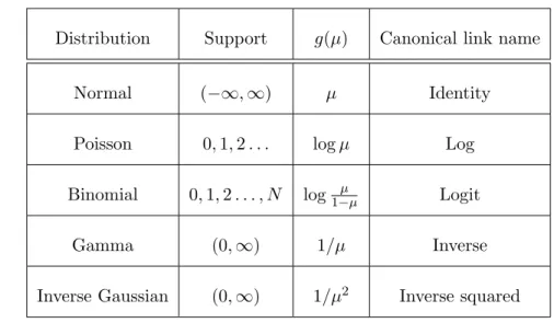
If the distribution from the exponential family is expressed in terms of its mean µi, such that θi =g(µi) for a given function g(·), theng(·) is referred to as the canonical link function. The canonical link function is the default link function used in GLMs, but it is not mandatory. Although the canonical link function can provide desirable statistical properties, non-canonical link functions can be used if they provide a better fit for the data or if they can better explain the model and the coefficients. Table1.1provides a summary of the canonical link function for some common distributions that are members of the exponential family. The link function is linearly related to the predictors in the model such that

g(E[Y]) =g(µ) =Xβ=η.

In order to obtain the mean of the model, one can invert the link function as follows:

E[Y] =g−1(Xβ) =g−1(η).

Note that with GLMs, one does not transform the response variable, but rather the mean of the response variable. Therefore, a model where logY is linearly related to the predictors (Eq. IV) is not the same model where GLM is used with a log link function, where in the latter logE[Y]

is linear on the predictors (Eq. V).

logyi=β0+β1xi1+. . .+βpxip+i (IV) logE[yi] =β0+β1xi1+. . .+βpxip+i. (V)

(22)

Table 1.1: Characteristics of some common exponential family members as shown byMcCullagh

(1984).

Distribution Support g(µ) Canonical link name

Normal (−∞,∞) µ Identity

Poisson 0,1,2. . . logµ Log

Binomial 0,1,2. . . , N log₁₋µ_µ Logit

Gamma (0,∞) 1/µ Inverse

Inverse Gaussian (0,∞) 1/µ2 Inverse squared Example: Poisson Distribution

The canonical link function for the Poisson distribution is obtained by finding g(·), where θ=g(µ). By observing Eq. 1.2.4, we have that θ= logµ, therefore, the canonical link function for the Poisson distribution is g(µ) = logµ.

Example: Gamma Distribution

The canonical link function for the Gamma distribution is obtained by finding g(·), where θ=g(µ). By observing Eq. 1.2.5, we have thatθ=−1/µ, therefore the canonical link function for the Gamma distribution is g(µ) =−1/µ. This canonical link function is equivalent to the inverse link function, which is shown as follows:

g(µi) =− 1 µ = p X j=1 xijβj. Therefore, 1 µ = p X j=1 xij(−βj) = p X j=1 xijβj∗,

(23)

whereβ_j∗=−βj. However, this does not enforce positive means for the model. Thus, it is more common to use the log link functiong(µ) = log(µ) for data that requires positive values.

To obtain the model parameters, we can use the maximum likelihood estimation method, where we differentiate the negative log-likelihood with respect to the parameter of interest β. The likelihood function of a distribution that is a member of the exponential family and has a density function as in Eq. 1.2.1is defined as

L(θ, φ;Y) = n Y i=1 exp yiθi−b(θi) ai(φ) +c(yi, φ) ,

and its log-likelihood is

l(θ, φ;Y) = n X i=1 yiθi−b(θi) ai(φ) +c(yi, φ) . (1.2.6)

The maximum likelihood estimate ˆβis obtained by solving the following system of equations ∂l(θ, φ;Y)

∂βj

= ∂l ∂βj

= 0.

However, our parameter of interestβj is not explicit in Eq. 1.2.6. But we know the following µi=b0(θi), ηi =

p X

j=1

xijβj, g(µi) =ηi. By applying the chain rule, we have that

∂l ∂βj = n X i=1 ∂l ∂θi · ∂θi ∂µi ·∂µi ∂ηi · ∂ηi ∂βj , where ∂l ∂θi =−yi−b 0_(θ i) ai(φ) =−yi−µi ai(φ) ∂θi ∂µi = 1/∂µi ∂θi = 1/∂b 0_(θ i) ∂θi = 1/b00(θi) ∂µi ∂ηi = 1/∂ηi ∂µi = 1/ ∂ ∂µi g(µi) = 1/g0(µi)

(24)

∂ηi ∂βj = ∂ ∂βj p X j=1 xijβj =xij. Therefore, we obtain ∂l ∂βj =− n X i=1 (yi−µi)xij ai(φ)b00(θi)g0(µi) .

By using Eq. 1.2.3, the above formula can be simplified into ∂l ∂βj =− n X i=1 (yi−µi)xij V ar[Yi]g0(µi) .

There are no closed form solutions for all GLM models. Therefore, numerical optimization is performed using computer software. The most common technique is Iterative Weighted Least Squares (IWLS), followed by Fisher scoring method and Newton Raphson method as explained byMcCullagh(1984).

The interpretation of model parameters for the GLM models is slightly different than that of the OLS coefficients. Consider a GLM model with a log link function and only one covariate, then it can be expressed as follows:

logE[Y|X] =β0+β1X ⇔ E[Y|X] = exp (β0+β1X). (1.2.7)

Therefore, if we increase the value of the covariate by 1, the log of E[Y|X] increases by β1 as

follows:

logE[Y|X+ 1] =β0+β1(X+ 1)

logE[Y|X+ 1] =β0+β1X+β1.

However, we are not interested in the change of the log of the mean ofY, but rather the change of the mean ofY. Therefore, by applying Eq. 1.2.7, we have that

logE[Y|X+ 1] =β0+β1X+β1 ⇔ E[Y|X+ 1] = exp (β0+β1X+β1)

= exp (β0+β1X) exp (β1)

=E[Y|X] exp (β1). (1.2.8)

So exp(β1) is a multiplicative factor that represents the increase due to a 1 unit increase in X,

(25)

1.2.5 Assumptions

Similar to OLS, there are some assumptions that should hold in order to use GLMs, or to choose the distribution used in the modeling. Breslow(1996) explained all the assumptions needed for GLMs and they are summarized in this section.

Assumption 6. Correct choice for all components of the GLM.

The distribution used in the modeling should be well suited for the data. For example, if we are observing an outcome variable that is positive, continuous and rightly skewed, the Gamma distribution can be a good choice. However, if we are modeling an outcome variable that is discrete and represents count of events, then the Poisson distribution can be a good choice. Additionally, the link function should be chosen to well represent the data. For example, if we are modeling positive outcomes, the link function should be chosen such that its inverse would always result in positive mean values.

Assumption 7. The observations in the data set are independent and sampled randomly such that the number of observationsy1, . . . , yn are bigger than the number of parameters β.

Independence of the observations is one of the important assumptions because it assures that we have a model with only fixed effects, and no random effects. We explore the changes in the model for data that has random effects in Section1.3. In addition, if the number of observations nis equal to the number of parametersp, then we have equal number of equations as unknowns, which can be solved algebraically. Ifn < p, then no unique solution is available.

Assumption 8. The predictors are non-random.

The predictorsxi1, . . . , xipare assumed to have fixed values such that variation in the predictors causes variation in the outcomeyi. However, changes in the outcome should not imply changes in the predictors. In other words, if we are modeling the amount of auto insurance losses, then it is assumed that the amount of the loss depends on the car type, but the car type does not depend on the amount of the loss.

Assumption 9. Multi-collinearity should be minimized.

There should be “almost” no linear relationship between the predictors. If there is a strong linear relationship (Pearson correlation coefficient ρp close to ±1) between the predictors, we should drop some of them such that the chosen model has “almost” uncorrelated predictors.

(26)

By estimating the parameters of the GLM model, we can obtain the fitted values ˆy which are generally not equivalent to the original data valuesy, with the goal to obtain small differences between them. McCullagh(1984) mentioned that there are several measures used to calculate that difference and they use the log-likelihood function illustrated in Eq. 1.2.6.

Consider the following:

• l(ˆθ, φ;Y) represents the maximized log-likelihood of the fitted model for a fixed value of the dispersion parameterφ,

• l(˜θ, φ;Y) represents the log-likelihood from the saturated model, a hypothetical model, where each observation is perfectly fitted without errors, and

• l(θ0, φ;Y) represents the log-likelihood from the null model, a hypothetical model, with

only an intercept value and no predictors such that every observation is estimated by the mean.

The predictions from the saturated model, ˜yi, exactly match the actual observations,yi. For this model, each observation has its own parameters, i.e. there are nestimates for ˜β, and therefore, each estimate perfectly predicts the value of the outcome. The saturated model can be observed as the upper bound of the log-likelihood function, because it theoretically provides the best fit, while the null model is the lower bound of the log-likelihood function. The maximized model has a log-likelihood value in between those bounds.

The discrepancy of the fit is measured by obtaining the difference between the saturated model and the fitted model, which gives us a quantity named the scaled deviance, defined as follows:

D∗(ˆθ, φ;Y) = 2 h

l(˜θ, φ;Y)−l(ˆθ, φ;Y) i

.

By using Eq. 1.2.6, and ai(φ) =φ/ωi we can rewrite the scaled deviance of the model as D∗(ˆθ, φ;Y) = 2 " _n X i=1 " yiθ˜i−b(˜θi) ai(φ) +c(yi, φ) # − n X i=1 " yiθˆi−b(ˆθi) ai(φ) +c(yi, φ) ## = 2 " _n X i=1 " yiθ˜i−b(˜θi) φ/ωi +c(yi, φ)− yiθˆi−b(ˆθi) φ/ωi +c(yi, φ) ##

(27)

= 2 φ n X i=1 ωi h yi ˜ θi−θˆi −b(˜θi)−b(ˆθi) i , (1.2.9)

where the deviance of the model is defined as D(ˆθ, φ;Y) = 2 n X i=1 ωi h yi ˜ θi−θˆi −b(˜θi)−b(ˆθi) i , (1.2.10)

and the quantityD∗(ˆθ, φ;Y) is simply the deviance scaled by the dispersion parameter φ. The values ofD(ˆθ, φ;Y) and D∗(ˆθ, φ;Y) are always positive since the saturated model has a higher log-likelihood value than any fitted model, and their values will approach 0 when the fitted parameters perfectly explain the model without errors.

Example: Poisson Distribution

The deviance for the Poisson distribution is obtained by using previous results that we obtained in earlier examples. Since θ = logµ, and b(θ) = exp{θ} for the Poisson distribution and by assuming equal priori weightsωi = 1, then the deviance from Eq. 1.2.10 becomes

D(ˆθ, φ;Y) =D( ˆµ;Y) = 2 n X i=1 ωi[yi(logyi−log ˆµi)−(yi−µˆi)] = 2 n X i=1 yilog yi ˆ µi −(yi−µˆi) .

The scaled deviance for the Poisson distribution is the same as the deviance because the disper-sion parameter φ= 1.

Example: Gamma Distribution

Similar to the Poisson distribution, obtaining the deviance for the Gamma distribution relies on previous results that we obtained in earlier examples. Sinceθ=−1/µandb(θ) =−log(−θ) for the Gamma distribution and by assuming equal priori weights ωi = 1, then the deviance from Eq. 1.2.10becomes D(ˆθ, φ;Y) =D( ˆµ;Y) = 2 n X i=1 ωi yi ₋₁ yi −−1 ˆ µi −(logyi−log ˆµi) = 2 n X i=1 yi−µˆi ˆ µi −log yi ˆ µi .

The scaled deviance for the Gamma distribution is obtained by scaling the deviance by the dispersion parameterφsuch thatD∗(ˆθ, φ;Y) = D(ˆθ,φ_φ;Y).

(28)

It is important to mention that when log-likelihoods or deviance is used to compare models, this comparison is only valid when the compared models are done over the same data set with the same number of observations. This is because the log-likelihood is obtained by summing the log-likelihoods for each observation, and if a model has more observations than another model, then it will have a higher log-likelihood value, which should not be attributed to having a better fit to the data. It is also important to use deviance only in comparing models that have the same distribution and the same dispersion parameter, i.e. everything in the model should be identical except the coefficients. This is because the deviance measures the deviation from the log-likelihood of the saturated model. Therefore changing any assumptions in the model other than the coefficients would change the value of the log-likelihood of the saturated model, not only the fitted model, which makes the comparison between models by using the deviance obsolete. If the distribution of a model is a special case from another model, such as the Poisson distribution being a special case of the Negative Binomial distribution, then it is appropriate to use the deviance as a model selection criteria.

Additionally, a model M1 is said to be nested of another model M2 if it uses a subset of the

predictors of M2. If we want to compare the two nested models M1 and M2 with p1 and p2

number of predictors respectively, such thatp2> p1, and parameters ˆθ1 and ˆθ2 respectively, we

can use the scaled deviance (or deviance) of each model to obtain a likelihood ratio test statistic as follows: D∗(ˆθ1, φ;Y)−D∗(ˆθ2, φ;Y) = 2 h l(ˆθ2, φ;Y)−l(ˆθ1, φ;Y) i = 2 lnl(ˆθ2, φ;Y) l(ˆθ1, φ;Y) .

This statistics asymptotically follows the Chi-Square distribution with degrees of freedom ν = p2−p1.

Frequently, we would like to compare models that are not nested, or from different exponential families, and hence comparing their deviance is not an accurate goodness of fit test because of reasons mentioned earlier. In that case, we will have to refer to other model selection criteria which will be explored later in Chapter3.1.

(29)

1.3 Generalized Linear Mixed Models

Sometimes it occurs that the observations in the data are not independent, for example, longi-tudinal data where repeated observations of the same variables are measured over time for the same individual, or when the data is obtained from groups (countries, hospitals, schools, etc.). This adds a random effect to the model, which makes GLM no longer applicable. Generalized Linear Mixed Models (GLMMs) are an extension of GLMs where random effects are added to the model, in addition to the usual fixed effects available in GLMs. The term “mixed model” implies the use of both fixed and random effects in the modeling. Random effects are always associated with categorical variables, which divides the data into several groups. For example, assume we want to model and make statistical inference about the amount of auto insurance losses in Canada, and the data is collected from several insurance companies. For each com-pany, we will obtain the amount of the losses Y, and the predictors X which includes age and profession of the insured, car model, etc. If the companies represent the entire population, (i.e. we collected data from all companies in Canada), then we would want to focus our analysis on the effect of each company and on its impact on the loss amount. Therefore, the parameters for each company are considered model parameters, and not random variables, hence, the com-pany is a fixed effect. However, if the companies represent a sample of the population (i.e. we collected data from some companies in Canada), we will be interested in knowing the trend for the entire population, not just those sampled companies. Therefore, the parameters of those companies are no longer considered fixed model parameters; they are random variables and thus have probability distributions. Hence, we will be interested in knowing the variance between the companies, in order to make a general conclusion about the population. The distinction between the companies being considered a population versus samples is what distinguishes a model with fixed effects and random effects, respectively.

1.3.1 The Model

Consider a sample of N independent multivariate response Yi = (yi1, . . . , yin)T such that i= 1, . . . , N, where yij is thejth response for theith group/subject. For simplicity of notation, it is assumed that each group has the same number of observationsn. We assume that each response yij depends on a p×1 vector of fixed predictors xij associated with a vector of fixed effects coefficients β and on a q×1 vector of fixed predictors zij associated with a vector of random

(30)

effects coefficientsbi = (b0i, b1i, . . . , bqi)T. Given the random effectb, the mean of the response vectorY is assumed to be related to the predictors via an arbitrary link function g(·) such that

g(E[Y|b]) =g(µ|b) =Xβ+Zb,=η,

where it is assumed thatb∼N(0,G), whereG is the variance-covariance matrix of the random effects. Note that the random effects help in identifying the variation of each sample/group from the population mean (or the fixed effects), so imposing a mean of zero makes the model unique, and we are interested in estimating the variance. Similar to the GLMs, in order to obtain the mean of the model, one can invert the link function g(·).

To help us explain the above model, we will assume an intercept, only 1 covariate Xij and 3 groups/subject. The expanded matrices become:

                        η11 .. . η1n η21 .. . η2n η31 .. . η3n                         =                         1 .. . 1 1 .. . 1 1 .. . 1                         β0+                         x11 .. . x1n x21 .. . x2n x3n .. . x3n                         β1+                         1 0 0 .. . ... ... 1 0 0 0 1 0 .. . ... ... 0 1 0 0 0 1 .. . ... ... 0 0 1                              b01 b02 b03      +                         x11 0 0 .. . ... ... x1n 0 0 0 x21 0 .. . ... ... 0 x2n 0 0 0 x3n .. . ... ... 0 0 x3n                              b11 b12 b13      , or h X0 X1 i   β0 β1  + h Z0 Z1 i   b0 b1  ,

where X0 is a (n×N)×1 vector of ones, X1 is a (n×N)×1 vector with elements equal

to the covariateXij for the corresponding observation,β0 and β1 are the regression coefficients

for X0 and X1, respectively. Z0 is an (n×N) ×3 matrix whose ij component is 1 if the

corresponding observation is in the ith group/subject, and 0 otherwise. Z1 is an (n×N)×3

matrix whose elements are Xij if the corresponding observation is from the ith group/subject and 0 otherwise. ηij is represented by

(31)

= (β0+b0i) + (β1+b1i)xij,

whereb0i explains the deviation from the intercept,β0, for theithgroup, andb1iis the deviation from the slope of X1,β1 for theith group. In addition,

b=   b0 b1  ∼N     0 0  ,   Iσ2₀ Iσ10 Iσ01 Iσ21    .

Conditional on the random effectsb, the responses Y are assumed to be mutually independent and generated from the same exponential family as explained in Section1.2.2.

Similar to GLMs, Maximum likelihood estimation is also used to estimate the fixed effects coefficientsβ in GLMMs. In addition, it is also used to estimate the random effects coefficients b and G, the variance of the random effects. Stroup (2012) provided detailed explanation on obtaining the model parameters, and they also confirm on the difficulty of obtaining closed form solutions for the estimates, and hence computer software are used for numerical optimization.

Please refer to Chapter3.1for details on assessing the goodness of fit of the model and compar-ison between models.

(32)

Chapter 2

Multivariate Models

The univariate models provide a variety of methods to model data sets that have only one outcome variable Y. However, we often need to model several outcomes and to observe the dependency between them. A multivariate distribution is a distribution that has more than one random variable linked together through a dependence structure. This dependence structure explains if they are independent or dependent on each other, and also the direction and strength of the dependence. This chapter presents the properties of multivariate distribution functions and their relationship with copulas. We also explore the fundamentals of copulas and their use in statistical modeling.

Note that in this section, we work with the assumption that each random variable is a continuous random variable, but some of the notations and properties can be translated to discrete variables by using summands instead of integrands. However, some notations have complicated forms for discrete distributions, especially in copulas.

2.1 Multivariate Distribution Functions

Consider the random vectorX which contains n random variables X1, . . . , Xn linked together through a joint density function f and joint distribution function F. The support of each random variable Xi is RXi = [Li, Ui], which is the set of values that the random variable can take. For the rest of this chapter, we will assume that the lower limit Li =−∞ and the upper limitUi =∞,∀i= 1, . . . , n. Consider a set of observations {x1, . . . , xn} ∈ Rn, then their joint

(33)

distribution functionF is defined by

F(x1, x2, . . . , xn) =P(X1≤x1, . . . , Xn≤xn).

The relationship between the joint probability density function (pdf) and the joint cumulative distribution function (cdf) is defined by

F(x1, . . . , xn) = Z x1 −∞ · · · Z xn −∞ f(x1, . . . , xn) dxn· · ·dx1, and f(x1, . . . , xn) = ∂n ∂x1· · ·∂xn F(x1, . . . , xn). (2.1.1) For a function to be defined as multivariate pdff, it has to satisfy the following properties:

• f(x1, . . . , xn)≥0, • R∞

−∞. . .

R∞

−∞f(x1, . . . , xn) dxn· · ·dx1 = 1, and

• ifA⊂Rn is a set of values for X, then

P[(X1, . . . , Xn)∈A] = Z · · · Z A f(x1, . . . , xn) dxn· · ·dx1.

In addition, the multivariate cdfF has the following properties:

• F(x1, . . . , xn) is non-decreasing, i.e. if any of the xi increases, then F(x1, . . . , xn) also increases,

• If all components approach their maximum attainable value, then the value of the cdf F is equal to 1, i.e.

lim x1,...,xn→∞

F(x1, . . . , xn) = 1,

• If one or more components approach their minimum attainable value, then the value of the cdf F is equal to 0, i.e. ,∀i= 1, . . . , n,

lim xi→−∞

F(x1, . . . , xn) = 0,

• and if∀(a1, . . . , an),(b1, . . . , bn)∈[0,1]n whereai ≤bi, we have the rectangle inequality

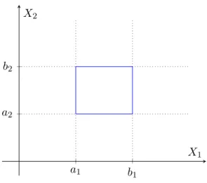
2 X i1=1 . . . 2 X in=1 (−1)i1+...+id_F_(x 1i1, . . . , xnin)≥0, wherexj1 =aj andxj2=bj ∀j∈1, . . . , n.

(34)

a1 b1

a2

b2

X1

X2

Figure 2.1: Illustration of the rectangle inequality for a bivariate distribution

The last property might not be trivial for an-dimensionalX, but it ensures thatP(a1 ≤X1≤

b1, . . . , an ≤ Xn ≤ bn) is non-negative. A simple example of the rectangle property can be explained by Figure2.1which assumes a bivariate cdf, then visualizing a rectangle with vertices (a1, a2),(b1, a2),(a1, b2) and (b1, b2) where 0≤a1 ≤b1 ≤1 and 0≤a2 ≤b2 ≤1, then

F(b1, b2)−F(a1, b2)−F(a2, b1) +F(a1, a2)≥0.

If one wishes to work with each random variableXi separately, then we have the marginal pdf and cdf,fXi(x) and FXi(x), respectively. They are obtained as follows:

fXi(x) = Z ∞ −∞ · · · Z ∞ −∞ f(x1, . . . , xn) dx1· · ·dxi−1dxi+1· · ·dxn, FXi(x) = lim x1,...,xi−1,xi+1,...,xn→∞ F(x1, . . . , xn).

In addition, the random variablesX1, . . . , Xn are independent if and only if f(x1, . . . , xn) =fX1(x1)· · ·fXn(xn),

F(x1, . . . , xn) =FX1(x1)· · ·FXn(xn). (2.1.2) The conditional pdf and cdf of Xi given the other variables Xi−, where X_i− represents the

random vectorX ={X1, . . . , Xn}without the random variable Xi, are given by fXi|Xi−(xi|xi−) = f(x1, . . . , xn) fXi(xi) , (2.1.3) FXi|Xi−(xi|xi−) = F(x1, . . . , xn) FXi(xi) . (2.1.4)

(35)

Additionally, the multivariate survival function ¯F is defined by ¯

F(x1, x2, . . . , xn) =P(X1> x1, . . . , Xn> xn).

2.2 Copulas

Any multivariate distribution function for a vector of random variables can implicitly describe the marginal distribution functions and their dependence structure. However, with the limited availability of known multivariate distribution functions and the complexity of modeling real data by using them, one is inclined to use copulas. In this section, we define copulas, explain their properties and identify their link with multivariate cdfs. We also provide examples of spe-cific families of copulas. Joe(1997,2014) andMcNeil et al.(2015) provided detailed explanation for copulas and dependence modeling.

Copulas provide a mean to model the dependence relationship between two or more random variables. The n-dimensional copula is a multivariate cdf on [0,1]n with standard uniform marginal distributions. Let X = (X1, . . . , Xn) be a random vector which contains n random variables linked through the cdf F. Set Ui = Fi(Xi) ∼ U(0,1), i = 1, . . . , n, where Fi(Xi) is the marginal cdf of the random variable Xi. Hence, the copula C is a mapping of the form C: [0,1]d→[0,1] and is defined by

C(u1, . . . , un) =P(U1 ≤u1, . . . , Un≤un), ui ∈[0,1], i= 1, . . . , n. (2.2.1) The following properties must hold for any copulaC:

• C(u1, . . . , un) is increasing in each of its components, i.e. if any of the ui increases, then C also increases,

• C(1, . . . ,1, ui,1, . . . ,1) = ui,∀i ∈ 1, . . . , n. This property holds due to the uniform marginals,

• C(1, . . . ,1) = 1, i.e. if all components reach their maximum attainable values, then the value of the copulaC is 1,

• C(u1, . . . , ui−1,0, ui+1, . . . , un) = 0, i.e one or more components are at their minimum attainable values, then the value of the copulaC is 0, and

(36)

• ∀(a1, . . . , an),(b1, . . . , bn)∈[0,1]n whereai ≤bi we have the rectangle inequality 2 X i1=1 . . . 2 X in=1 (−1)i1+...+id_C(u 1i1, . . . , unin)≥0, whereuj1 =aj anduj2=bj ∀j∈1, . . . , n.

The above properties, except the second one, are the same properties identified for any multi-variate cdf as explained in Section2.1.

Sklar(1959) defined the link between copulas and multivariate cdfs, but the following proposi-tions must be defined first.

Proposition 2.2.1. Let F be a distribution function andF−1 denote its inverse, i.e. F−1(y) = inf{x:F(x)≥y}, then

1. Quantile Transformation. If U ∼U(0,1), then P F−1(U)≤x=F(x),

2. Probability Transformation. If X∼F where F is continuous, then F(X)∼U(0,1). This leads us toSklar’s Theorem, which proves that all multivariate cdfs can be written in terms of copulas and that copulas can be used with the marginal cdfs to obtain a multivariate cdf.

Theorem 2.2.2. Sklar’s Theorem Let F be a n-dimensional distribution function with mar-gins F1, . . . , Fn. Then there exists a couplaC : [0,1]n→[0,1]such that ∀x1, . . . , xn∈R

F(x1, . . . , xn) =C(F1(x1), . . . , Fn(xn)),

where Fi(xi) is the marginal distribution function of Xi,∀i ∈ 1, . . . , n. Conversely, if C is a copula and Fi(xi) are the marginal distribution function of Xi,∀i∈1, . . . , n, then

C(F1(x1), . . . , Fn(xn)) =F(x1, . . . , xn),

where F is a multivariate cdf with margins F1, . . . , Fn. Additionally, if the margins are contin-uous, thenC is unique; otherwise, if one or more of the marginals is discrete, thenC is unique only on RanF1×. . .×RanFn, where RanFi denotes the range ofFi, and RanF1×. . .×RanFn represents the cartesian product of the ranges.

(37)

Proof. We provide the proof for the continuous case. For the detailed proof, please refer to

Nelsen(1999).

Consider the continuous random vectorX = (X1, . . . , Xn) with a multivariate cdf F, which can be represented as

F(x1, . . . , xn) =P(X1 ≤x1, . . . , Xn≤xn)

=P(F1(X1)≤F1(x1), . . . , Fn(Xn)≤Fn(xn)). (2.2.2) By using the Probability Transformation defined in Proposition 2.2.1, we have that Fi(Xi) = Ui ∼ U(0,1). Then Eq. 2.2.2 corresponds to the cdf of (F1(X1), . . . , F1(X1)) = (U1, . . . , Un). We introduce a functionC, called a copula, such that

P(F1(X1)≤F1(x1), . . . , Fn(Xn)≤Fn(xn)) =C(F(x1), . . . , F(xn)) IfF is evaluated at the arguments xi =Fi−1(ui),0≤ui≤1,∀i= 1, . . . , n, then,

C(u1, . . . , un) =F F₁−1(u1), . . . , Fn−1(un)

. (2.2.3)

Since F is continuous, then Eq. 2.2.3 provides an explicit form for the copula in terms of the cdfF and its marginsFi, which proves it is unique.

Contrarily, assume thatC is a copula and that Fi,∀i= 1, . . . , n are the univariate cdfs, where Xi =F_i−1(Ui). Let U ∼C, then F(x1, . . . , xn) =P(X1≤x1, . . . , Xn≤xn) =P F₁−1(U1)≤x1, . . . , Fn−1(Un)≤xn =P(U1 ≤F1(x1), . . . , Un≤Fn(xn)) =C(F1(x1), . . . , Fn(xn)) =F(x1, . . . , xn).

The pdf of the copulaC can be calculated by using 2.1.1as follows: c(u1, . . . , un) =

∂n ∂u1. . . ∂un

(38)

Hence, the pdf of the random vectorX is f(x1, . . . , xn) = ∂nF(x1, . . . , xn) ∂x1· · ·∂xn = ∂ n_C(F 1(x1), . . . , Fn(xn)) ∂x1· · ·∂xn = ∂ n_C(F 1(x1), . . . , Fn(xn)) ∂F1(x1)· · ·∂Fn(xn) ∂F1(x1) ∂x1 · · ·∂Fn(xn) ∂xn =c(F1(x1), . . . , Fn(xn))f1(x1)· · ·fn(xn). (2.2.4) Even though the n-dimensional copula is the general case, to avoid cumbersome notation, we will restrict our discussion to the bivariate random vector X = (X1, X2) with observations

x1, x2, and its associated copulaC(F1(X1), F2(X2)). All the properties and discussions can be

generalized to then-dimensional copula.

The survival copula is defined by ¯C F¯1(x1),F¯2(x2)

, where ¯Fi(xi) is the survival function of the random variableXi, ∀i∈1,2. ¯C is derived as follows:

¯ C F¯1(x1),F¯2(x2) = ¯F(x1, x2) = 1−F1(x1)−F2(x2) +F(x1, x2) = 1−F1(x1)−F2(x2) +C(F1(x1), F2(x2)) = ¯F1(x1) + ¯F2(x2)−1 +C(1−F¯1(x1),1−F¯2(x2)). Therefore, ¯ C(u1, u2) =C(1−u1,1−u2) +u1+u2−1. (2.2.5)

The conditional copula ofU2 given U1 =u1 is defined by

CU2|U1(u2|u1) =P(U2 ≤u2 |U1 =u1) = lim h→0P(U2≤u2 |u1≤U1 ≤u1+h) = lim h→0 C(u1+h, u2)−C(u1, u2) P(U1 ≤u1+h)−P(U1 ≤u1) = lim h→0 C(u1+h, u2)−C(u1, u2) h = ∂ ∂u1 C(u1, u2). (2.2.6)

(39)

Similarly,C_U₁|U2(u1|u2) =

∂

∂u2C(u1, u2).

Example: FGM Copula

Assume a bivariate distribution F(X1, X2), whereXi ∼Exp(βi) where βi >0, ∀i= 1,2, such that

F(x1, x2) = (1−e−β1x1)(1−e−β2x2)

+θ(1−e−β1x1₎₍₁₋_e−β2x2_)e−β1x1_e−β2x2_,

with dependence parameter−1≤θ≤1, to be discussed later in Section 2.3. The corresponding copulaC can be obtained by finding the inverse ofFi(xi) = 1−e−βixi =ui, which isFi−1(ui) = −_β1

i ln(1−ui) =xi. By replacing each xi with the inverse in the above bivariate distribution, we obtain

C(u1, u2) =u1u2+θu1u2(1−u1)(1−u2). (2.2.7)

The pdf of the copulaC is

c(u1, u2) = ∂2 ∂u1∂u2 C(u1, u2) = ∂ 2 ∂u1∂u2 u1u2+θu1u2(1−u1)(1−u2) = 1 +θ(1−2u1)(1−2u2). (2.2.8)

The joint density function is

f(x1, x2) =c(F1(x1), F2(x2))f1(x1)f2(x2) = (1 +θ(1−2F1(x1))(1−2F2(x2)))β1e−β1x1β2e−β2x2 = 1 +θ(1−2e−β1x1₎₍₁₋_2e−β2x2₎ β1e−β1x1β2e−β2x2.

The survival copula is ¯

C(u1, u2) =C(1−u1,1−u2) +u1+u2−1

= (1−u1)(1−u2) +θ(1−u1)(1−u2)u1u2+u1+u2−1

=u1u2+θu1u2(1−u1)(1−u2). (2.2.9)

Note that for the FGM, the survival copula ¯C is equivalent to the copula C, which makes it a symmetric copula.

(40)

The conditional copula ofU2 given U1 =u1 is CU2|U1(u2|u1) = ∂ ∂u1 C(u1, u2) = ∂ ∂u1 [u1u2+θu1u2(1−u1)(1−u2)] =u2+θu2(1−2u2)(1−u2).

Furthermore, the copulaC is bounded as per the following theorem:

Theorem 2.2.3. Fr´echet-Hoeffding copula bounds For any bivariate copula C and u = {u1, u2} ∈[0,1]2, we have the following bounds

W(u1, u2)≤C(u1, u2)≤M(u1, u2), (2.2.10)

where W(u1, u2) = max(u1+u2−1,0) and M(u1, u2) = min(u1, u2).

Proof. Upper bound: IfC is the cdf of (U1, U2), thenC(u1, u2) =P(U1 ≤u1, U2 ≤u2).

Given that P(U1 ≤u1, U2 ≤u2)≤P(U1 ≤u1) andP(U1 ≤u1, U2 ≤u2)≤P(U2 ≤u2), then P(U1≤u1, U2 ≤u2)≤min(P(U1 ≤u1), P(U2 ≤u2)) ≤min(u1, u2). Lower bound: P(U1 > u1, U2 > u2) = 1−P(U1 ≤u1)−P(U2 ≤u2) +P(U1 ≤u1, U2 ≤u2) = 1−u1−u2+C(u1, u2)≥0.

Therefore, by rearranging the above inequality,C(u1, u2)≥u1+u2−1.

Note thatM(u1, . . . , un) is a copula for any value ofn, however, W(u1, . . . , un) is only a copula forn= 2. M andW are referred to as the comonotonic and countermonotonic copulas, respec-tively. They will be discussed further in Section2.2.1.

(41)

The empirical estimator of a copula is defined as Cn(u1, u2) = 1 n n X i=1 1{Fn1(Xi1)≤u1,Fn2(Xi2)≤u2}, (2.2.11)

whereFnj is the empirical cdf of Xj = (x1j, . . . , xnj), such that Fnj(t) = 1 n n X i=1 1{xij≤t}. 2.2.1 Families of Copula

In this section, we explore different families of copulas and their properties. The most common families of copulas are

• Perfect dependence and independence copulas, • Elliptical copulas,

• Archimedean copulas, and • Extreme-value copulas.

Perfect Dependence and Independence Copulas

Independence Copula

The random variablesX1 and X2 are independent if and only if

C(u1, u2) =u1u2.

This is equivalent to Eq. 2.1.2. The independence copula has the following notation: Π(u1, u2).

Comonotonicity Copula

X1 =φ(X2) almost surely (a.s.) for an increasing functionφ(·) if and only if

C(u1, u2) = min(u1, u2).

The comonotonicity copula is the upper Fr´echet-Hoeffding copula presented in Theorem 2.2.3. X1 and X2 are perfectly positively dependent because they are a.s. strictly increasing functions

(42)

Countermonotonicity Copula

X1 =ψ(X2) almost surely (a.s.) for a decreasing function ψ(·), if and only if

C(u1, u2) = max(u1+u2−1,0).

The countermonotonicity copula is the lower Fr´echet-Hoeffding copula presented in Theorem 2.2.3. X1 and X2 are perfectly negatively dependent because they are a.s. strictly decreasing

functions of each other.

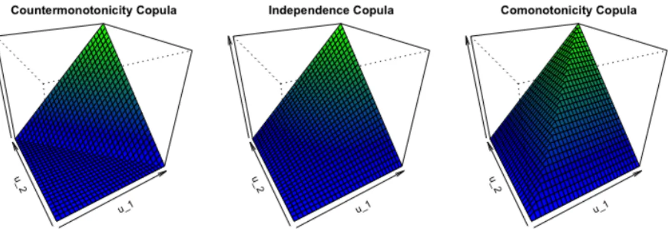
Figure2.2 illustrates the perspective plots of the cdfs of the dependence copulas and the inde-pendence copula. The Fr´echet-Hoeffding bounds presented in Theorem2.2.3imply that the cdf of all bivariate copulas lie between the surfaces of the Countermonotonicity and Comonotonicity copulas.

Figure 2.2: Perspective plots of the cdf of the Countermonotonicity copula, Independence copula and Comonotonicity copula.

Elliptical Copulas

An elliptical copula is a generalization of the multivariate Gaussian distribution. They do not have a closed form expression, but they are extracted from the multivariate cdfs by using Sklar’s Theorem2.2.2.

(43)

Gauss Copula

IfX = (X1, X2) follows a standardized bivariate Gaussian distribution, then

C_ρGauss(u1, u2) = Φρ Φ−1(u1),Φ−1(u2)

,

where Φ is the cdf of a standard univariate normal random variable and Φρ is the cdf of a bivariate normal random variable with mean 0 and correlation ρ ∈[−1,1]. The Gauss copula does not have an explicit form, but it can be represented as the integral over the pdf of X as follows: C_ρGauss(u1, u2) = Z Φ−1(u1) −∞ Z Φ−1(u2) −∞ 1 2πp1−ρ2 exp −x 2₊_y2₋_2ρxy 2(1−ρ2₎ dydx. Student’st-Copula

IfX = (X1, X2) follows a bivariate Student’st-distribution, then

C_ν,ρt (u1, u2) =tν,ρ tν−1(u1), t−ν1(u2)

,

wheretν is the cdf of a standard univariate t-distribution with ν degrees of freedom,tν,ρ is the cdf of a bivariate t-distribution with mean 0, correlation ρ ∈ [0,1] and ν degrees of freedom. ν determines the thickness of the tails of the t-distribution; the more the degrees of freedom, the lighter the tails, and vice verse. The t-copula does not have an explicit form, but it can be represented as the integral over the pdf ofX as follows:

C_ν,ρt (u1, u2) = Z t−ν1(u1) −∞ Z t−ν1(u2) −∞ 1 2πp1−ρ2 1 +x 2₊_y2₋_2ρxy ν(1−ρ2₎ dydx.

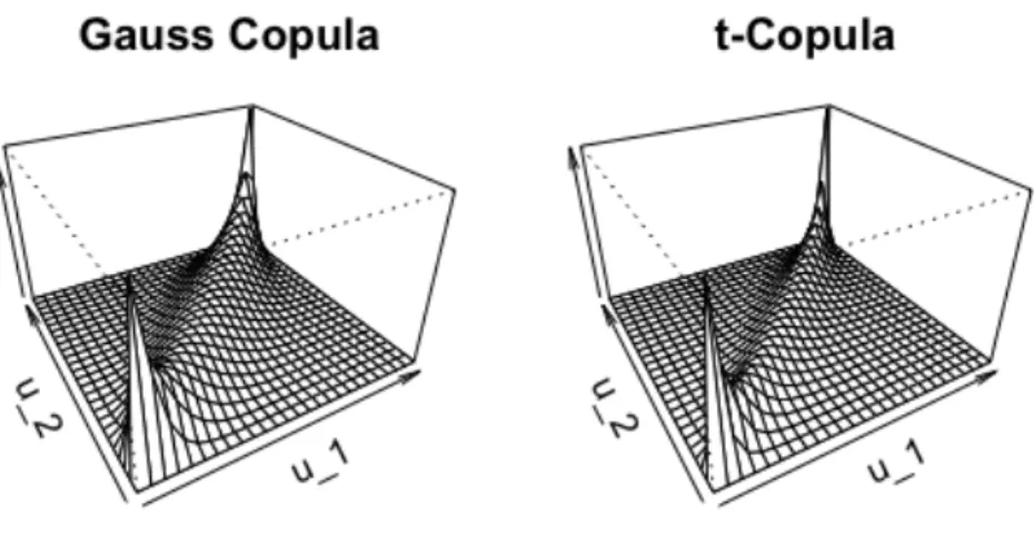
We can observe from Figure2.3that the t-copula assigns more probability mass to the corners of the unit square, which means they have heavier tails than the Gauss copula. This character-istic for thet-copula can be altered by changing the degrees of freedomν. Note that if we had assumed no correlation, i.e. ρ= 0, then this would result in independence, and hence, there will be no higher mass in the corners.

(44)

Figure 2.3: Perspective plots of the densities of the bivariate Gauss copula with ρ= 0.9238795 and bivariatet-copula with ρ= 0.9238795 andν = 2.

Figure 2.4: Top: One thousand simulated points from the Gaussian copula with ρ= 0.9238795 and bivariatet-copula with ρ= 0.9238795 andν = 2.

Bottom: Realizations of X1 and X2 by assuming standard normal marginals for the copulas

(45)

The top row of Figure2.4 represents 1000 simulated points from the Gauss andt-copulas. For the bottom row, we assume that (X1, X2) has standard normal marginals, so each simulated

point from the copula is transformed component-wise into standard normal. The parameters are chosen such that both copulas have the same value of Kendall’s tau, to be discussed in Section 2.3. Other elliptical copulas include the Cauchy copula and the Pearson Type II copula.

Archimedean Copulas

Unlike the elliptical copulas defined in Section 2.2.1, Archimedean copulas have closed forms. In this section, we define bivariate Archimedean copulas and provide examples for it. For mul-tivariate Archimedean copulas, refer toMcNeil and Neˇslehov´a (2009) andMcNeil et al.(2015).

A bivariate Archimedean copula has the form

Cθ(u1, u2) =φ−1[φ(u1;θ) +φ(u2;θ) ; θ], (u1, u2)∈[0,1]2, θ∈Θ, (2.2.12)

whereφ : [0,1]×Θ→ R+ is a strictly decreasing convex function with dependence parameter

θ. The function φ is called the generator function of the copula, and its inverse is represented byφ−1. In addition, φ(0) =∞and φ(1) = 0. Table2.1summarizes the generator functions and other details for the most commonly used Archimedean copulas.

Bivariate Clayton Copula

Consider the generator φ(t;θ) = 1_θ t−θ−1, where θ ≥ −1 and t ∈ [0,1]. The inverse of the generator is represented by φ−1(t;θ) = (1 +θt)−1/θ. By using the general form of the Archimedean copula represented in Eq. 2.2.12, we obtain the bivariate Clayton copula

C_θCl=u−₁θ+u₂−θ−1−1/θ, θ≥ −1.

The bivariate Clayton copula is characterized by the following limiting cases: • Countermonotonicity copula whenθ=−1 (only in the bivariate case), • Independence copula whenθ→0, and

(46)

Bivariate Frank Copula

Consider the generator φ(t;θ) = −ln

e−θt−1 e−θ₋₁

, where θ∈ _R and t ∈[0,1]. The inverse of the generator is represented by φ−1_(t;_{θ) =} ₋1

θln

1 + e−t _e−θ₋₁

. By using the general form of the Archimedean copula represented in Eq. 2.2.12, we obtain the bivariate Frank copula as follows: C_θF r=−1 θln " 1 + e −θu1₋₁ _e−θu2 ₋₁ e−θ₋₁ # .

The bivariate Frank copula is characterized by the following limiting cases • Countermonotonicity copula whenθ→ −∞(only in the bivariate case), • Independence copula whenθ→0, and

• Comonotonicity copula whenθ→ ∞.

Bivariate Gumbel Copula

Consider the generator φ(t;θ) = (−lnt)θ, where θ ≥ 1 and t ∈ [0,1]. The inverse of the generator is represented by φ−1(t;θ) = e−t1/θ. By using the general form of the Archimedean copula represented in Eq. 2.2.12, we obtain the bivariate Gumbel copula as follows:

C_θGu = exp

−h(−lnu1)θ+ (−lnu2)θ

i1/θ .

The bivariate Gumbel copula is characterized by the following limiting cases • Independence copula whenθ= 1, and

• Comonotonicity copula whenθ→ ∞.

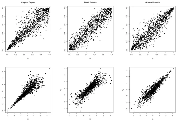
Figures2.5and2.6provides an example of each of the Archimdean copulas discussed previously. We can observe that the Clayton copula and the Gumbel copula provide strong lower and upper tail dependence, respectively. However, the Frank copula provides symmetry along both tails.

(47)

Figure 2.5: Perspective plots of the densities of the bivariate Clayton copula, bivariate Frank copula, and bivariate Gumbel copula. The dependence parameter for each copula is θ= 6,14.1385 and 4, respectively.

Figure 2.6: Top: One thousand simulated points from the Clayton, Frank and Gumbel copulas with dependence parameter for each copula isθ= 6,14.1385 and 4, respectively.

Bottom: Realizations of X1 and X2 by assuming standard normal marginals for the copulas

(48)

The Archimedean family offers a great deal of flexibility, however they have some limitations that prevent them from modeling asymmetric dependence relationships. Those limitations are

• C is symmetric, i.e. C(u1, u2) =C(u2, u1), ∀(u1, u2)∈[0,1]2, and

• C is associative, i.e. C(C(u1, u2), u3) =C(u1, C(u2, u3)), ∀(u1, u2, u3)∈[0,1]3.

Table 2.1: Summary of the generators φ(t), where t∈[0,1], the possible values for the depen-dence parameterθ, and the limiting cases for some bivariate Archimedean copulas.

Copula φ(t) θ Lower Limit Upper Limit

C_θCl= u−₁θ+u−₂θ−1 −1/θ 1 θ t −θ₋₁ θ≥ −1 W(u1, u2) M(u1, u2) C_θF r=−1 θln 1 +(e −θu1−1)(e−θu2−1) e−θ₋₁ −lne_e−−θtθ₋−₁1 θ∈_R W(u1, u2) M(u1, u2) C_θGu = e−[(−lnu1)θ+(−lnu2)θ] 1/θ (−lnt)θ θ≥1 Π(u1, u2) M(u1, u2) Extreme-value Copulas

Rare events need careful modeling because they might have a serious impact on the dependence structure of the distribution. This gives importance to extreme-value copulas. Gudendorf and Segers(2010) provided detailed explanation on the origin and properties of those copulas. Note that extreme-value copulas have complicated forms for dimensions >2.

Bivariate extreme-value copulas have the form CA(u1, u2) = exp ln(u1u2)A ln(u2) ln(u1u2) , whereA: [0,1]→[1/2,1] is a convex mapping such that

max(t,1−t)≤A(t)≤1, t∈[0,1].

Gumbel’s First Asymmetric Model

This is a generalization of the Gumbel Copula from the Archimedean family presented in Section 2.2.1. For this copula, A(t) is given by

A(t) = (1−α)t+ (1−β)(1−t) + h

(αt)θ+ (β(1−t))θ i1/θ

(49)

This copula is defined as Cθ(u1, u2) =u11−βu1 −α 2 exp −h(−βlnu1)θ+ (−αlnu2)θ i1/θ .

Note that if α=β = 1, we obtain the Gumbel Copula.

Gumbel’s Second Model

For this copula,A(t) is given by

A(t) =θt2−θt+ 1, θ∈[0,1]. This copula is defined as

Cθ(u1, u2) =u1u2exp ln(u1) ln(u2) ln(u1) + ln(u2) .

Galambos Asymmetric Copula For this copula,A(t) is given by

A(t) = 1−h(αt)−θ+ (β(1−t))−θi−1/θ, θ∈[0,∞)α, β∈[0,1]. This copula is defined as

Cθ(u1, u2) =u1u2exp −h(−βlnu1)−θ+ (−αlnu2)−θ i−1/θ . 2.2.2 Vine Copula

Vines were originally introduced byBedford and Cooke(2002) as a graphical model for high di-mensional distributions that have conditional dependence. Assuming we have 3 random variables (X1, X2, X3), Figure2.7illustrates thatf(x1|x2) andf(x3|x2) are dependent with a conditional