The Heart Defect Analysis Based on PCG Signals Using Pattern Recognition Techniques

(1)

Procedia Technology 24 ( 2016 ) 1024 – 1031

ScienceDirect

Peer-review under responsibility of the organizing committee of ICETEST – 2015 doi: 10.1016/j.protcy.2016.05.225

International Conference on Emerging Trends in Engineering, Science and Technology (ICETEST

- 2015)

The Heart Defect Analysis Based on PCG Signals

Using Pattern Recognition Techniques

Lubaib.P

a

*

, Ahammed Muneer KV

b

a

Post Graduate Student, Government Engineering College ,Kozhikode, India

b

Assistant Professor, Government Engineering College,Kozhikode, India

Abstract

The graphical recording of the heart sounds and murmurs is called Phonocardiogram or PCG and the machine is so called phonocardiograph. It has an important role in the proper and accurate diagnosis of the heart defects. It requires highly and experienced professionals to read the phonocardiogram, as usually with the stethoscope. The paper is about the implementation of a diagnostic system as a detector and classifier; for heart diseases. Various heart sound samples are classified using Support Vector Machine (SVM), K Nearest Neighbour (KNN), Bayesian and Gaussian Mixture Model (KNN) Classifiers. The output of the system is the classification of the sound as either normal or abnormal and if it is abnormal, what type of abnormality is present. In the proposed method, time domain and frequency domain features are extracted. Various frequency domain features such as energy, mean, variance and Mel Frequency Cepstral Coefficients (MFCC) are analysed.

Peer-review under responsibility of the organizing committee of ICETEST – 2015. Keywords: Phonocardiogram; features; systole; diastole; MFCC; SVM; KNN; KNN

* Corresponding author. Tel.:+91 9745465434; 8943214939

E-mail address: [email protected]

(2)

1.Introduction

Cardiovascular diseases are seriously threatening to human health. The significant percentages of the people who die due to cardiovascular diseases belong to rural part. The major reasons are lack of awareness, lifestyle, and the cost factor. Heart sound analysis is significant for diagnosing different kinds of cardiovascular diseases. More than 90% of heart murmurs in children are innocent. In cardiac auscultation, an examiner uses a stethoscope to listen for these sounds, which give important information about the condition of the heart.

Heart is one of the important organs in our body, which pumps blood continuously throughout the entire life-time. Heart is made up of a strong muscle called myocardium, and has four valves for controlling the blood circulation. Heart beats in regular intervals and is controlled by the electrical pulses generated from the sinus node near the heart. The rhythmic beating of heart sound referred to as “Lub-Dub” due to the closing of the atrio -ventricular and the aortic-pulmonic valves. Moreover, there are other sounds, which are due to the structural and functional defects of the heart, called as murmurs. Since all these sound generated is related to the physiology of the heart valves and muscles, analysis of heart sounds provides valuable information regarding the functioning of heart. Stethoscope is still used as the primary auscultation device for heart and lung sounds. Frequently the skills of the first examiner are not adequate to differentiate between innocent and pathological murmurs. However, analysis

using a stethoscope is depends on the doctor’s experience and hearing ability.

The purpose of this study is to develop an algorithm for Peak Spacing Analysis for Estimating Arrhythmic Heart-Beat, Based on this; each and every cycle of the PCG signals is separated into four parts: the first heart sound, the systolic period, the second heart sound and the diastolic period. This information and the intervals of the systolic and diastolic period are obtained consequently. Then the systolic and diastolic both the periods are analysed separately as well as in combined manner. Then based on this study the heart signal are analysed whether the sound is arrhythmic or not. If it is arrhythmic then, whether it is overall arrhythmic or the systolic and diastolic periods are arrhythmic.

2.Background

The history of auscultation, or listening to the sounds of the body, is easily described by a few evolutionary leaps. Hippocrates (460-377 BC) provided the foundation stone for auscultation when he put his ear on the chest of a patient and described the sounds he could hear from it. The next step was made by Robert Hooke (1635-1703) who realized the diagnostic use of cardiac auscultation. Although Dr. Laennec's invention, the stethoscope, has been in clinical use for more than 180 years, and electronic stethoscopes with variable gain have been available for over 80 years. The phonocardiogram, first developed in 1894, visualizes auscultatory signals. The spectral phonocardiogram has proven to be a reliable tool that gives information of whether or not the murmur is pathological. During the past few years, however, the improvements of personal computers have made it possible to design new low-cost, high quality phonocardiographic devices. Spectral phonocardiography emulates the ear and may be ideal for teaching clinical stethoscopy. The phono-spectrogram combines traditional phonocardiogram with time-frequency distribution presentation of the signal. The spectrogram was introduced for heart sound analysis as early as 1955 by McKusik et al, but was afterwards almost forgotten. The stethoscope (from the Greek word stethos, meaning “chest” and skopein, “to examine”)invented during the early 20 th century, was one of the most primitive devices designed to aid a doctor in listening to heart sounds. It was a simple tool used for transmitting the sound energy from the chest wall of the patient to the ear of the physician via a column of air. The 20thcentury witnessed extraordinary advances in the diagnosis of heart diseases, corrective surgeries, and other forms of treatment for heart problem.

3.Methodology

The Phonocardiogram (PCG) could be used as a simple and effective source for analyzing and detecting the arrhythmic nature of heart beat. The heart rhythm is directly related to the electrical activity of the heart as well as

(3)

its valve movements. The data used in this paper was obtained from Michigan university website. The following methodology has been employed to study the effectiveness of PCG in cardiac diagnosis.

3.1.Pre-Processing

The recorded heart sound signal is required to pre process before envelope extraction. The heart sound signals were normalized according to the equation (1) as shown below.

ݔnormሺݐሻ = ቀ

௫ሺ௧ሻ ୫ୟ୶ȁ௫ሺ௧ሻȁቁ

ଶ

(1) Where x(t) is the original signal and the square operation leads to make peak signal more prominent and weaken the noise.

3.2.Envelope Detection

The envelope of the heart sound signal can be detected using squared energy of the signal [5], the squared energy method based on exponential weighing factors to high intensity components.

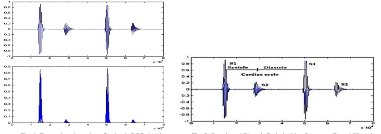
Square Energy E = x2 (2) Fig. 1.shows the energy based envelop of a simple PCG signal which is convenient to find S1 and S2 locations.

3.3.Separation of Systole and Diastole

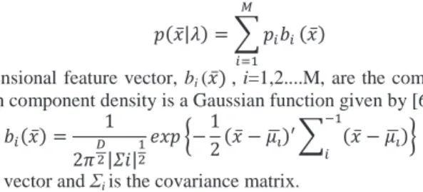
To identify peaks, there is a need to formalize an algorithm to automatically detect peaks in any given time-series. A data point in a time-series is a local peak if it is a large and locally maximum value with respect to all other data points in a window. By identifying peak-locations and peak-amplitude values in a phonocardiogram wave located the S1 and S2 peaks. It has been observed that S1-peak values are normally larger than S2-peak values. The time-gap between consecutive S1 and S2 peaks represents systole period whereas the time-gap between consecutive S2 and S1 peaks measured as diastole period. Every systole and diastole periods are recorded along the entire sample sequence for further analysis. The time gap between two S1 peaks called cardiac cycle, which includes one systole and diastole. All these are shown in Fig. 2.

From the separation of systole and diastole it is easy to calculate systolic period, diastolic period, heart rate etc. Then total phonocardiogram wave of one minute duration is split into many cardiac cycles. Every systole and diastole periods, cardiac cycles are recorded along the entire sample sequence for further analysis

(4)

3.4.Feature extraction

Automatic extraction of features depends on accurate knowledge about the timing of the heart cycles. Segmentation into the first heart sound (S1), systole, the second heart sound (S2) and diastole is thus needed. In this paper, both time domain and frequency domain features are extracted. The database used for feature extraction is heart sound samples from Michigan University website.

3.4.1.Time domain Features

The envelope of heart sound was extracted with the normalized average energy, the heart sound signal was divided into each cardiac cycles. Each cardiac cycle was divided into short overlapping segments of fixed and equal duration. Energy was calculated in each segment and which is recorded and plotted as shown in Fig. 3. Energy of corresponding segments in each cardiac cycle is stored in an array, and calculated their mean and variance.

3.4.2.Frequency domain Features

There are so many transforms available to obtain frequency domain features. In this paper Mel Frequency Cepstral Coefficients (MFCC) are used as frequency domain features [1],[3]. MFCCs are a way of representing the spectral information in a sound. Each coefficient has a value for each frame of the sound. The changes within each coefficient across the range of the sound are examined here. MFCC are good features for better classification accuracy. Obtaining the MFCCs involves analysing and processing the sound according to the following steps

x Divide the signal into frames

x Obtain the amplitude spectrum of each frame

x Take the log of these spectrums

x Convert these to the Mel scale

x Apply the Discrete Cosine Transform (DCT).

The computation of the MFCC includes Mel-Scale filter-banks, as shown in Fig. 4. The Mel-Scale filter-banks are computed as follows:

݉ ൌ ͳͳʹ͹݈݋݃௘൬ ݂

͹ͲͲ൅ ͳ൰ሺ͵ሻ

Where f is the frequency in the linear scale and m is the resulting frequency in Mel-Scale.

The power spectral density (PSD) of the spectrum is mapped onto the Mel-Scale by multiplying it with the filter-banks constructed earlier and the log of the energy output of each filter is calculated as follows[1],[2]:

ݏሾ݉ሿ ൌ ݈݋݃ ൭෍ ȁܺሾ݇ሿȁଶ

ேିଵ

௞ୀ଴

ܪ௠ሾ݇ሿ൱ሺͶሻ

(5)

where Hm[k] is the filter-banks and m is the number of the filter-bank. Finally, to obtain the MFCC the discrete

cosine transform (DCT) of the spectrum is computed:

ܿሾ݊ሿ ൌ ෍ ܵሾ݉ሿ ቆߨ݊ ܯ൬݉ െ ͳ ʹ൰ቇ ேିଵ ௠ୀ଴ ǡ ݊ ൌ Ͳǡͳǡʹ ǥ Ǥ Ǥ ܯሺͷሻ

Where M is the total number of filter banks.

3.5.Classification

3.5.1.Support Vector Machine(SVM)

After the feature extraction process, support vector machine was used to classify the data. Support Vector Machines (SVM) [1],[2],[3] is a binary learning machine with some highly elegant properties. The foundations of Support Vector Machines (SVM) have been developed by Vapnik (1995) .The main idea of support vector machine is to construct a hyper plane as the decision surface in such a way that the margin of separation between positive and negative examples is maximized.

Consider the training sampleሼሺݔ௜ǡ ݀௜ሻሽ_௜ୀଵே ǡ where xi is the input pattern for the i

th

example and di is the

corresponding desired response. Assume that the pattern represented by the subset di = +1 and the pattern

represented by the subset di = -1 are linearly separable. The equation of the decision surface in the form of a hyper

plane that does the separation is

்ܹ_{ܺ ൅ ܾ ൌ Ͳሺ͸ሻ}

Where X is the input vector, W is an adjustable weight vector, and b is a bias. Thus we can write

்ܹ_{ܺ ൅ ܾ ൒ Ͳ݂݋ݎ݀}

௜ൌ ൅ͳሺ͹ሻ

்ܹܺ ൅ ܾ ൏ Ͳ݂݋ݎ݀௜ൌ െͳሺͺሻ

For a given weight vector w and bias b , the separation between the hyper plane defined in Equation and the closest data point is called the margin of separation, denoted by. The goal of support vector machine is to find the particular hyper plane for which the margin of separation is maximized. Under this condition, the decision surface is referred to as the optimal hyper plane. Fig. 5 illustrates the geometric construction of an optimal hyper plane for a two dimensional input space

Let w0 and b0 denote the optimum values of the weight vector and bias, respectively. Now the optimal

hyper plane is

ܹ଴்ܺ ൅ ܾ଴ൌ Ͳሺͻሻ

The discriminant function

݃ሺݔሻ ൌ ܹ଴்ܺ ൅ ܾ଴ൌ ͲሺͳͲሻ

gives an algebraic measure of the distance from x to the optimal hyper plane. The particular data points (xi; di) for

which

ܹ଴்ܺ ൅ ܾ଴ൌ ൅ͳ݂݋ݎ݀௜ ൌ ൅ͳሺͳͳሻ

ܹ଴்ܺ ൅ ܾ଴ൌ െͳ݂݋ݎ݀௜ൌ െͳሺͳʹሻ

(6)

satisfied are called support vectors, hence the name support vector machine. In conceptual terms, the support vectors are those data points that lie closest to the decision surface and are therefore the most difficult to classify. The optimum value of the margin of separation

ߩ ൌ_ԡݓʹ

଴ԡሺͳ͵ሻ

The optimum value of weight vector and bias is determined using Lagrange optimization theory.

ܹ଴ൌ ෍ ߙ଴ǡ௧

௡

௧ୀଵ

݀௜ݔ௜ሺͳͶሻ

where ߙ଴ǡ௧ is the optimum Lagrange multipliers.

ܾ଴ൌ ͳ െ ܹ଴்ܺሺ௔ሻ݂݋ݎ݀ሺ௔ሻൌ ͳሺͳͷሻ

Where X(s) is a support vector.

3.5.2.Bayesian Decision Theory

Bayesian decision theory is a fundamental statistical approach to the problem of quantifying pattern classification [13]. This approach is based on decisions using probability Bayes formula can be expressed informally.

ܲ݋ݏݐ݁ݎ݅݋ݎ ൌ݈݈݄݅݇݁݅݋݋݀ ൈ ݌ݎ݅݋ݎ

݁ݒ݅݀݁݊ܿ݁ ሺͳ͸ሻ

The minimum error rate classification can be achieved by maximizing the discriminant function using Bayes formula.

݃௜ሺݔሻ ൌ ݌൫ݓ௜ൗ ൯ ൌݔ ݌൫ݔ ݓ௜

ൗ ൯Ǥ ݌ሺݓ௜ሻ

σ஼௜ୀଵ_{݌൫ݔ ݓ}ൗ ൯Ǥ ݌ሺݓ_௜ ௜ሻ

ሺͳ͹ሻ

Where ݌൫ݓ௜ൗ ൯_ݔ is the posterior probability of ݓ௜with respect to x, ݌൫ݔ ݓൗ ൯_௜ is the likelihood of ݓ௜with respect to

x,݌ሺݓ௜ሻ is the prior probability ofݓ௜. Maximizing the discriminant function gives,

݃௜ሺݔሻ

ൌ

݌൫ݔ ݓൗ ൯Ǥ ݌ሺݓ_௜ ௜ሻሺͳͺሻ

Applying logarithm on equation gives,

݃௜ሺݔሻ ൌ ݈݊ܲ ൬

ݔ

ݓ௜൰ ൅ ݈݊ܲሺݓ௜ሻሺͳͻሻ

This expression can be readily evaluated if the densities ݌ ቀ_௪௫

೔ቁare multivariate normal, In this case, then,

݃௜ሺݔሻ ൌ ൬ ͳ ʹ൰ ሺݔ െ ߤ௜ሻ்෍ ሺݔ െ ߤ௜ሻ ିଵ ௜ ൬ ݀ ʹ൰ ݈݊ʹߨ െ ݈݊ȁߑȁ ൅ ݈݊ܲሺݓ௜ሻሺʹͲሻ 3.5.3.K-Nearest Neighbour(KNN)

The k Nearest Neighbour (KNN) method is a widely used technique in clustering and classification applications [13]. In this method given that a set of N points (training set), whose class labels are known, classify a set of n points (testing set) into the same set of classes by examining the k closest points around each point of the testing set and by applying the majority vote scheme. k-NN is a type of instance-based learning, or lazy learning, where the function is only approximated locally and all computation is deferred until classification. The k-NN algorithm is among the simplest of all machine learning algorithms. The neighbours are taken from a set of objects for which the class (for k-NN classification) or the object property value (for k-NN regression) is known.The algorithm has nothing to do with and is not to be confused with k-means, another popular machine learning technique

(7)

3.5.4.Gaussian Mixture Model(GMM)

Gaussian Mixture Model (GMM) belongs to the stochastic modeling and it is based on the modeling of statistical

variations of the features [11].Mixture density in GMM is the weighted sum of M component densities and is given

by the equation,

݌ሺݔҧȁߣሻ ൌ ෍ ݌௜ܾ௜ ெ

௜ୀଵ

ሺݔҧሻሺʹͳሻ

Where, x is a D-dimensional feature vector, bi (ݔҧሻ , i=1,2....M, are the component densities and pi ,1,2....M are the

mixture weights.Each component density is a Gaussian function given by [6],

ܾ௜ሺݔҧሻ ൌ ͳ ʹߨ஽ଶȁߑ݅ȁଵଶ ݁ݔ݌ ൜െͳ ʹሺݔҧ െ ߤഥ ሻԢ ෍ ሺݔҧ െ ߤప ഥ ሻప ିଵ ௜ ൠሺʹʹሻ

Where, µi is the mean vector and Σi is the covariance matrix.

4.Result and Discussion

Heart sounds are analysed by the methodology mentioned above. To identify S1 and S2 peaks in the test signal, the peak-locations and peak-amplitude values are analysed from the energy envelop. And alsoS1, S2 peaks, heart beat per minute is calculated. Experimentally it has been observed that S1-peak values are normally larger than S2-peak values. The time-gap between consecutive S1 and S2 peaks represents systole period whereas the time-gap between consecutive S2 and S1 peaks is measured as diastole period, and also it has been observed that the period of Systole gap is always less than the diastole gaps. MFCC are extracted frequency domain features, based on these features KNN and SVM classifier is used to classify whether these signals are normal and abnormal. Mean and variance of average energy are extracted time domain features, based on these features Bayesian and GMM classifier is used to classify whether these signals are normal and abnormal, and more over which is used to check what type of abnormality is present. Classification accuracy of each method is shown in Table. 1 and in Table 2.Based on time domain features such as mean and variance of energy the heart sound signals are classified in to different types of common abnormalities by using Bayesian decision theory and Gaussian mixture model. The wave form of single cardiac cycle and its corresponding energies of each case are shown in figure below. The normal condition, that is no mummers present in systolic and diastolic period is shown in Fig. 6 Mitral Regurgitation, abnormality due to murmurs present in systolic period is shown in Fig. 7 Aortic Regurgitation, abnormality due to murmurs present in diastolic period is shown in Fig. 8Patent Ductus Arteriosus, abnormality due to murmurs present in systolic and diastolic period is shown in Fig. 9.

Fig. 6 Waveform and energy of normal condition Fig. 7 Waveform and energy of abnormal (Mitral Regurgitation)

(8)

Table I. Classifier with obtained accuracy Table II. Accuracy obtained using time domain features

Classifier Case Accuracy

SVM Linear kernel 98.97% Polynomial kernel(d=2) 99.98% Polynomial kernel (d=3)5 99.99% 99.80% KNN 5.Conclusion

Heart sounds are processed and analyzed by the processing steps mentioned above. From the energy envelop and S1, S2 peaks, heart beat per minute is calculated. Experimentally it has been observed that S1-peak values are normally larger than S2 peak values and also it has been observed that the time period of Systolic gap is always less than the diastolic gaps. It is concluded that the abnormality of heart sound is not only depend on the overall cardiac cycle whereas it depends upon the individual analysis of systolic and diastolic period. By the feature extraction of each cardiac cycle and classification mentioned above, it is concluded that whether the signal is normal or abnormal and what type of abnormality present. SVM with polynomial kernel (d=2 and d=3) and second case of Bayesian classifier obtained higher accuracy. The Heart defect detection with better accuracy using simple technique is achieved in this paper.

Acknowledgements

This paper will be incomplete without mentioning all the people who helped me to make this possible, whose encouragement was invaluable. I would like to thank Ahamed Muneer KV (Asst. Professor, AE&I), Abdul Rahiman (Asst. Professor, AE&I), Prof. Shajee Mohan B.S, Associate Professor, Department of Applied Electronics & Engineering for their committed guidance, valuable suggestions and encouragement.

References

[1] Behnam Farzam, Jalil Shirazi “ The Diagnosis of Heart Diseases Based on PCG Signals using MFCC Coefficients and SVM Classifier”

IJISET - International Journal of Innovative Science, Engineering & Technology, Vol. 1 Issue 10, December 2014

[2] X. J. Hu, J. W. Zhang, G. T. Cao, H. H. Zhu, and H. Li, “Feature extraction and choice in PCG based on hilbert transfer,” in Proc. 4th

International Congress on Image and Signal Processing (IEEE), 2011.

[3] Jithendra Vepa," Classification of heart murmurs using cepstral features and support vector machines" IEEE, 2009.

[4] .P. de Vos, and M. M. Blanckenberg, “Automated Pediatric CardiacAuscultation”, IEEE Trans. Biomed. Eng., Vol. 54, No. 2, (Febr. 2007),

pp. 244-252

[5] Study and Design of a Shannon-Energy-Envelope based Phonocardiogram Peak Spacing Analysis for Estimating Arrhythmic Heart-Beat,Praveen Kumar Sharma,Sourav Saha,Saraswati Kumari , International Journal of Scientific and Research Publications, Volume 4, Issue 9, September 2014 1 ISSN 2250-3153G.

[6] Heart Sound Analysis for Diagnosis of Heart Diseases in Newborns ,Amir Mohammad Amiri*, Giuliano Armano ,University of Cagliari, Department of Electrical and Electronic Engineering(DIEE), 09123 Cagliari, Italy ,ICBET 2013: May 19-20, 2013, Copenhagen, Denmark.

[7] Lubaib P,Ahammed Muneer KV and Abdu Rahiman VK “Phonocardiogram Based Diagnostic System” IJBES-International Journel of

Bimedical and Sceince 2015

[8] S. Cerutti, A. L. Goldberger, and Y. Yamamoto, “Recent Advances in Heart Rate Variability Signal Processing and Interpretation”, IEEE

Trans. Biomed Eng., Vol. 53, No.1 (Jan. 2006), pp. 1-3.

[9] C. N. Gupta, et al., “Segmentation and Classification of Heart Sounds,” CCECE/CCGEI, Saskatoon, IEEE, 1674-77, May2005.

[10] Jian-bo Wu, Su Zhou, "Research on the Method of Characteristic Extraction and Classification of Phonocardiogram", International Conference on Systems and Informatics, 2012.

[11] D.A. Reynolds, R.C. Rose, Robust text-independent speaker identification usingGaussian mixture speaker models, IEEE Trans. Speech Audio Process, 3 (1995) 72–83.

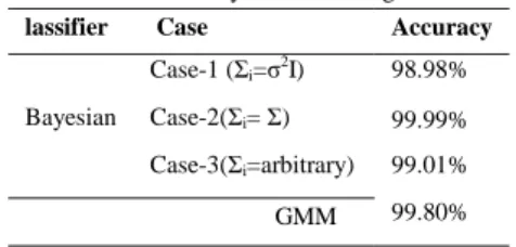
lassifier Case Accuracy

Bayesian Case-1 (Σi=σ2I) 98.98% Case-2(Σi= Σ) 99.99% Case-3(Σi=arbitrary) 99.01% 99.80% GMM