Line-source based X-ray Tomography
Deepak Bharkhada1,2, Hengyong Yu4, Hong Liu3, Robert Plemmons5, Ge Wang1,2,4 1. Biomedical Imaging Division, VT-WFU School of Biomedical Engineering &
Science, Wake Forest University, Winston-Salem, NC, 27157
2. Biomedical Engineering Department, Wake Forest University School of Medicine, Winston Salem, NC 27157
3. School of Electrical & Computer Engineering, University of Oklahoma, Norman, OK, 73019
4. Biomedical Imaging Division, VT-WFU School of Biomedical Engineering & Science, Virginia Tech., Blacksburg, VA, 24061
5. Departments of Mathematics and Computer Science, Wake Forest University, Winston-Salem, NC 27109
Abstract: Current computed tomography (CT) scanners, including micro-CT scanners, utilize a point x-ray source. As we target higher and higher spatial resolutions, the reduced x-ray focal spot size limits the temporal and contrast resolutions achievable. To overcome this limitation, in this paper we propose to use a line-shaped x-ray source so that many more photons can be generated, given a data acquisition interval. In reference to the simultaneous algebraic reconstruction technique (SART) algorithm for image reconstruction from projection data generated by an x-ray point source, here we develop a generalized SART algorithm for image reconstruction from projection data generated by an x-ray line source. Our numerical simulation results demonstrate the feasibility of our novel line-source-based x-ray CT approach and the proposed generalized SART algorithm.
Keywords: Computer tomography (CT), micro-CT, simultaneous algebraic reconstruction technique (SART), generalized SART, point source, line source.
I. Introduction
Since the first computed tomography (CT) scanner was made [1], all the commercial scanners have been employing the x-ray source with a small focal spot, which can be mathematically modeled as a point source. In micro-CT and even nano-CT applications, the reduced x-ray focal spot size has become a limiting factor to achieve desirable image resolution in terms of spatial, contrast and temporal measures. To address this issue, we propose to use a line-shaped x-ray source so that more photons can be generated in a given data acquisition interval. In this context, the x-ray source can be mathematically modeled as a line-segment. In point x-ray source CT scanners, the spatial resolution is limited by the finite focal-spot size necessary to generate a sufficient number of x-ray photons, and the temporal resolution is limited by the time necessary to acquire sufficient projection data over an angular range.
In contrast to recently proposed source configurations, like the multiplexed [2] and multiple-source geometry [3] which utilize multiple point x-ray sources to reduce the acquisition time, our technique treats the entire line segment as a single x-ray source. Since a line source covers a wide angular range per view, irradiation with an increased number of photons is achieved along with a relatively higher cooling capability of the x-ray source. Therefore, a line-shaped source technique could be a good candidate to balance among spatial, contrast and temporal resolution.
A line-shaped x-ray source can be fabricated using field emission x-ray source technology. Field emitters have been used as an electron sources for a long time. The most significant difference between the field emission x-ray tube and existing tubes lies in the field emitter cathode. The cathode can be made with an array of micro-machined field emission tips. By doing so, it is possible to obtain very sharp tips and very close proximity between the tips and the gate electrode. This greatly reduces the potential difference between the tip and the gate required to achieve the field emission. The array may also be very densely packed. As a result, even though the current that can be obtained from a single tip is small, the total current that can be obtained from an array can be much larger. Schwoebel et al. [4] reported that they were able to obtain a current of 300mA by packing 50,000 tips into a circular area of a square millimeter, which is equivalent to 40A/cm2. Using the technique as described above, a line shaped x-ray source can be fabricated. The width can be made as narrow as 0.01mm (or less), and the length of the source can be made in tens of centimeters or longer, if necessary.
The organization of this paper is as the follows. In the next section, we formulate a forward imaging model assuming a line source. In the third section, we develop a generalized simultaneous algebraic reconstruction technique (SART) to enable line-source-based reconstruction. In the fourth section, we perform numerical tests to demonstrate the performance of our technique. In the last section, we discuss relevant issues and conclude the paper.
II. Line-shaped X-ray Imaging Model
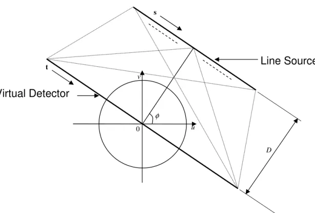
As shown in Fig. 1, a linear virtual detector is assumed in our line-shaped x-ray source acquisition geometry. Vectors s=(u,v) and t=(u,v) refer to the locations of the line-shaped x-ray source and the line detector, respectively. The x-ray forward projection model for a line source in terms of the number of photons arriving at a detector location
t can be written as ( ) ( , ) ( ) ( ) f ray dx O I N N e−∫ ∈ ds =
∫
x x s t t s , (1) where I(s)N is the original number of photons emanating from the source at a point s, )
(t
O
N is the number of photons arriving at a location t on the detector, x=(u,v) refers to a position along the x-ray path connecting points s and t, f(x) is linear attenuation coefficient of point x, x and s respectively represent the 1D coordinates along a fixed ray path and the line source, and the outer integral is carried out along the whole line
source. The power of the exponential term ( f dx ray( ,) ) ( t s x x ∈
∫
) is the line integral of theattenuation coefficients along the x-ray connecting points s and t.
If the length of the line is infinitesimally small, the x-ray attenuation model of a point source can be obtained by removing the outer integral in Eq. (1) as
( ) ( , ) ( ) ( ) f ray dx O I N N e−∫ ∈ = x x s t t s , (2) where s is the location of the point source and hence can assume only one value per view. Applying the logarithmic transformations on both sides of Eq. (2), we can obtain a linear equation representing the line integral of the attenuation coefficients along an x-ray path as
∫
∈ = − = f dx N N t p I ray O ) , ( ) ( ) ) ( ) ( log( ) ( x x st s t . (3) CT image reconstruction is a typical inverse problem of recovering f(x) from the corresponding forward projection models Eqs. (1) and (3). While there are many analytic algorithms for point-source projection data modeled by Eq. (3), the non-linear nature of Eq. (1) for the projection data of a line-shaped x-ray source makes it difficult to obtain a corresponding analytical method for the image reconstruction. However, an iterative method can be developed to achieve the reconstruction as demonstrated in the next section.III. Generalized SART algorithm
Although iterative methods have not been employed by any commercial CT scanners due to high computational costs associated with them, their superior performance is well established when the data is incomplete, noisy and dynamic. Meanwhile, there is a renewed interest in iterative algorithms due to the improvement in computational capabilities [5, 7]. It is well known that simultaneous algebraic reconstruction technique (SART) [6, 7] has remained a very powerful tool for iterative reconstruction since its introduction and it has been shown to converge to a weighted least squares solution from any initial guess [8]. Moreover, the SART method operates in the whole real space, while the other popular iterative algorithm expectation maximization is defined only for non-negative space, although it does preserve data fidelity for non-non-negative pixel and voxel values. Here, we will generalize the SART method for image reconstruction from projection data of the proposed line source model.
3.1 Point Source SART Algorithm
Because a projection for the point x-ray source is a linear integral of attenuation values along the x-ray path, (Eq. 3) it can be written in a discrete form as
∑
= ∆ = i J j ij i f x p 1 , (4)where
p
i is the ith projection, i =1,L,I with I being the number of projections given by the product of the number of views and the number of detector pixels, Ji is the number of sample points along the thi ray path,
f
ij are the attenuation coefficients of the points on the ith ray with j =1,L,Ji. Because most of the points along the x-ray pathsin Eq. (4) do not lie on the discrete image grid, it is necessary to obtain the attenuation values
f
ij for them from the image grid pixels via interpolation. Assuming that linear interpolation is employed, we can rewrite Eq. (4) as
∑
= ∆ = J j j ij i w f x p 1 ,∑
= = ∆ J j i ij x L w 1 , (5) wheref
j are the attenuation values of the image pixels, j=1,L,J with J being the number of pixels in the image,w
ij is the normalized weight contribution off
j on the image grid to the projectionp
i, Li is the length of the intersection between the ith x-ray path and support of the region being reconstructed.Let
a
ij=
w
ij∆
x
. Eq. (5) can now be simplified as
∑
= = J j j ij i a f p 1 . (6) This is equivalent to a linear system of equations given by
AF
=
P
, (7) whereA
is a I×J matrix,F
is a J×1 vector andP
is a I×1 vector with = IJ Ij I I iJ ij i i J j J j a a a a a a a a a a a a a a a a L K M O M L K M O M L K K L 2 1 2 1 2 2 22 21 1 1 12 11 A , (8) F=[f1,f2,L,fj,L, fJ]T, (9) P=[p1,p2,L,pi,L,pI]T. (10) The SART algorithm for solving
F
fromP
can be written in an iterative format as [7]
∑
∑
∑
= = = + − + = I i J j ij iter i i ij I i ij iter j iter j a p a a f f 1 1 1 1 1 ( aF ) , (11)where “ iter ” indicates the iteration number,
a
i is the ith row of matrixA
, and pi−a Fi iter is the ith difference between the real line integral and the line integral estimated from current image Fiter.3.2 Genearlized Line Source SART Algorithm
Following the same steps as for the point source, a projection for the line-shaped x-ray source based on Eq.(1) can be written in the discrete form as
N N f x s I i J j kij I i O k ik ∆ ∆ − =
∑
∑
= = ) exp( 1 1 , (12) whereNOK is the thk projection for the line source, k =1,L,Kwith K being the number of projections given by the product of the number of views and the number of detector pixels, I is the number of source points chosen for the discretization of the line source,
I i
N is the original number of photons in all x-rays from a line source point
i
, Nik is the number of sample points along the x-ray path from a line source pointi
to a detector pixel corresponding to the projectionk
, fkij is the linear attenuation coefficient of the points along the x-ray path from a source pointi
to a detector pixel corresponding to the projectionk
,∆
x
is the sampling interval along the ray path and ∆s is the sampling interval along the line source. In the following, we assume that all the x-rays from a line source have same original number of photons as NI.Although Eq. (12) is not a linear equation set, we can modify the SART algorithm to solve Eq. (12). Because most of the points on the x-ray paths in Eq. (12) do not lie on the discrete image grid, again it is necessary to obtain the attenuation values fkij for them
from the image grid pixels. Assuming that linear interpolation is employed, we rewrite Eq. (12) as N N w f x s I i J j j kij I O k ∆ ∆ − =
∑
∑
= = ) exp( 1 1 ,∑
= = ∆ J j ik kij x L w 1 , (13) wheref
j are the attenuation values of the image pixels, J is the number of pixels in the image, wkij is the normalized contribution of pixelf
j to the line-integral of theattenuation coefficients along the x-ray from a line source point
i
to the detector pixel corresponding to the projectionk
, andL
ik is the length of the intersection between the x-ray path from ith source point to the detector pixel corresponding to the projectionk
and the support of the region being reconstructed. Let oe
k or k k N N d = − )
exp( with Nkoe being
the estimated kth projection data and Nkor the real kth projection data, we have
oe k or k k N N d =−log . (14) The real projection data can now be rewritten in terms of the estimated projection data (Eq. (13)) as N d N w f x s I i J j j kij I k or k = −
∑
−∑
∆ ∆ = = ) exp( ) exp( 1 1 , (15) which can be simplified asN N w f x dk s I i J j j kij I or k =
∑
−∑
∆ + ∆ = = )) ( exp( 1 1 . (16) Again let akij =wkij∆x, Eq. (16) can be further simplified asN N a f dk s I i J j j kij I or k =
∑
−∑
+ ∆ = = )) ( exp( 1 1 . (17) Notice that the samed
k is added to the line integrals (∑
= J j j kijf a 1 ) of the attenuation coefficients along any x-rays from all the line source points to the detector pixel corresponding to the line source projection
k
.
Consider a hypothetical situation in which all the points along the line x-ray source serve as point x-ray sources and let qki denote the line integrals of the x-rays from these sources contributing to the projection
k
. Although the line integralsq
ik are not known, we will show in the following that it is not necessary to know them. Now we can form a linear system of equations
AF
=
Q
, (18) whereA
is a U×J matrix with U = K×I,F
andQ
are J×1 and U×1 vectors respectively described by = KIJ KIj KI KI KiJ Kij Ki Ki J K j K K K J K j K K K kIJ kIj kI kI kiJ kij ki ki J k j k k k J k j k k k IJ Ij I I iJ ij i i J j J j a a a a a a a a a a a a a a a a a a a a a a a a a a a a a a a a a a a a a a a a a a a a a a a a K L M O M L L M O M L L K L M M M M M M K L M O M L L M O M L L K L M M M M M M K L M O M L L M O M L L K L 2 1 2 1 2 2 22 21 1 1 12 11 2 1 2 1 2 2 22 21 1 1 12 11 1 1 2 1 1 1 1 1 2 1 1 1 12 12 122 121 11 11 112 111 A ’ (19) F=[f1,f2,L,fj,L, fJ]T, (20) Q=[q11,q12,L,q1i,L, q1I,L,qK1,qK2,L,qKi,L,qKI]T. (21) Along the rows of
A
andQ
, there are two index variablesi
andk
. If we combine them into one indexu
, we obtain = UJ Uj U U uJ uj u u J j J j a a a a a a a a a a a a a a a a L K M O M L K M O M L K K L 2 1 2 1 2 2 22 21 1 1 12 11 A , (22)
Q=[q1,q2, L ,qu, L ,qU]T. (23) At first look it appears that we can now use Eq. (11) only if
Q
is known as,
∑
∑
∑
= = = + − + = U u J j uj iter u u uj U u uj iter j iter j a q a a f f 1 1 1 1 1 ( a F ) . . (24)Notice that qu −a Fi iter is the difference between the real line integral qu and the line
integral a Fi iterestimated from the current iterate value Fiterof the image. This difference for a particular projection k is given by
d
k obtained in Eq. (14) thus making it unnecessary to know qu.To be consistent with indexing, let us also call
d
k asd
u while remembering thatu
is a combination of indexes
i
andk
and thatd
u is the same for all the x-rays (all i's) from the line-source for a particular projectionk
. We can now write Eq. (24) as
∑
∑
∑
= = = + + = U u J j uj u uj U u uj iter j iter j a d a a f f 1 1 1 1 1 . (25)Eq.(14) is the final SART algorithm for image reconstruction from the projection data of a line-shaped x-ray source. Because it can be applied for image reconstruction from any non-linear projection model, we call it a generalized SART algorithm.
IV. Numerical Simulations
To validate the feasibility of line-shaped x-ray source and demonstrate the merits of generalized SART algorithm, we developed a numerical simulator. The thorax Phantom [9] was used in our simulations. A 60 cm virtual linear detector was assumed and its detector element size was 0.1 cm. The center of the line source was at a perpendicular distance (D) (see Fig. 1) of 75 cm from the iso-center. The whole line source was rotated with the center of the line source tracing a circle of radius 75 cm. The source lengths of 3cm, 5cm, and 8cm were employed with projection data acquired for 160 equiangular views. Number of photons used per x-ray per source point was assumed to be107.
Numerical simulation results are presented in Figs. 2 to 5. The size of the images presented is 23.625 42× cm2 with 144 256× pixels. In Fig. 2, images are reconstructed at different number of iterations for a line source length of 3cm. Comparing Figs 2b, 2c, and 2d, it can be observed that the increasing the number of iterations images with sharper edges are obtained. This phenomenon is more obvious at the edges of the vertebra and the lungs. Image reconstructed after 100 iterations for the x-ray source lengths of 3cm, 5 cm, and 8 cm along with the column and the row profiles are presented in Figs. 3, 4 and 5 respectively. For our simulation cases the best image quality is obtained with a source length of 3 cm and relatively poor image quality is obtained with the source lengths of
3cm and 8cm. The increase in source length results in increased blurring especially at the edges. Thus, it becomes increasingly difficult to reconstruct fine structures which in our case are the ribs since they have sharp and thin boundaries.
V. Discussions and Conclusions
A point x-ray source used in commercial CT scanners limits the temporal and spatial resolution and also results in frequent heating of the x-ray tube. These limitations may be overcome by using the proposed line-shaped x-ray source based image technique. Reconstructing image from a line-shaped x-ray source is a challenging task due to non-linear nature of the resulting projection data. In this article, we developed a generalized SART algorithm to enable reconstruction from a line source. We believe that this algorithm can be easily extended to more general 1D x-ray source shapes and even to 2D planar x-ray sources as well, which may have applications in dynamic imaging. Moreover, the OS-SART algorithms [10] can be similarly modified to obtain a generalized OS-SART algorithm with faster convergence.
To the best of our knowledge, this is the first paper attempting to solve the contradiction between temporal and spatial resolutions by a non-point source. Additional research efforts are necessary along this direction. In this study we acquired projection data over an angular range of 2π , but it will be interesting to find out for practical reasons the minimum angular range necessary for reconstruction which may change for different source lengths. It will also be exciting to see if a finer sampling of x-ray source during numerical simulations improves spatial resolution. Although it has not been theoretically proved, we believe that the generalized SART is convergent to the real image value, as shown for SART in [8]. However, a detail study is beyond the scope of this paper but will provide additional insights into the performance of the algorithm.
There are also possibilities for enhancing our algorithm or developing new algorithms. In our view, the main limitation of our generalized SART algorithm is the blurring of the edges and a large number of iterations required to reconstruct sharp images. To this end, gradient or prior information may be incorporated within our algorithm or other algorithms utilizing gradient information could be developed in the future. Some examples of prior information include support and non-negativity constraints [11]. In addition, investigation of regularization approaches to alleviate noise magnification and blurring artifacts [12] is an important research direction to pursue in future work.
This is feasibility study and there is not enough information to comment on scatter and its effects. Scattering is a real concern in computed tomography and it will become important to study the amount of scatter and resulting image degradation as the line-shaped based x-ray source tomography advances. However, if needed, new algorithms could be developed to reduce the effects of scatter.
In conclusion, we proposed a novel line-shaped x-ray source based CT imaging technique and corresponding reconstruction method. The developed generalized SART algorithm enables image reconstruction from projection data of not only a line-shaped
x-ray source but also more generalized 1D and 2D source. Our numerical simulations have demonstrated the feasibility and merits of the proposed techniques and algorithms. Some interesting future research directions were also presented.
Acknowledgements
This work was partially supported by NIH/NIBIB grants (EB002667,EB004287 and EB007288).
References
1. Hounsfield, G.N., Computerized Transverse Axial Scanning (Tomography).1. Description Of System (Reprinted From British-Journal-Of-Radiology, Vol 46, Pg 1016-1022, 1973). British Journal Of Radiology, 1995. 68(815): p. H166-H172. 2. Zhang, J., et al., Multiplexing radiography for ultra-fast computed tomography: A
feasibility study. Medical Physics, 2007. 34(6): p. 2527-2527.
3. De Man, B., et al. Multi-source inverse geometry CT: a new system concept for x-ray computed tomography. in Medical Imaging 2007: Physics of Medical
Imaging. 2007. San Diego, CA, USA: SPIE.
4. Schwoebel, P.R., C.A. Spindt, and C.E. Holland, High current, high current density field emitter array cathodes. Journal of Vacuum Science &
Technology B (Microelectronics and Nanometer Structures), 2005. 23(2): p. 691. 5. Jiang, M. and G. Wang, Convergence studies on iterative algorithms for image
reconstruction. IEEE Transactions On Medical Imaging, 2003. 22(5): p. 569-579. 6. Andersen, A.H. and A.C. Kak, Simultaneous Algebraic Reconstruction Technique
(Sart) - A Superior Implementation Of The Art Algorithm. Ultrasonic Imaging, 1984. 6(1): p. 81-94.
7. Kak, A.C., Stanley, M, Principles of Computerized Tomographic Imaging.. 2001: Society of Industrial and Applied Mathematics.
8. Jiang, M. and G. Wang, Convergence of the simultaneous algebraic
reconstruction technique (SART). IEEE Transactions On Image Processing, 2003.
12(8): p. 957-961.
9. Sourbelle, K. Thorax Phantom, Available at:
http://www.imp.uni-erlangen.de/phantoms/thorax/thorax.htm. [cited 12/2/2007].
10. Ge, W. and J. Ming, Ordered-subset simultaneous algebraic reconstruction techniques (OS-SART). Journal of X-Ray Science and Technology, 2004. 12(3): p. 169.
11. Chen, D. and Plemmons, R., Nonnegativity Constraints in Numerical Analysis. Proceedings of the Symposium on the Birth of Numerical Analysis, Leuven Belgium, World Scientific Press, A. Bultheel and R. Cools, Eds., to appear 2009. 12. Persons, T., Hemler, P., and Plemmons, R., 3D Iterative Restoration of
Tomosynthetic Images, Integrated Computational Imaging Systems, OSA Technical Digest Series (Optical Society of America) 2001.
D u v
Line Source
Virtual Detector
s tFigure 1: Line x-ray source acquisition geometry
0
a b
c d
Figure 2: Comparison of images reconstructed using Line-SART algorithm using a line source of length 3 cm at different iteration numbers. a) Original Image. Reconstructed images in a), b) and c) are
respectively at 30, 60, and 100 iterations. Display window is [0.8, 1.2]
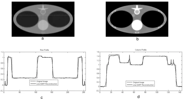
Figure 3: Line SART reconstructed images after 100 iterations using a line source of length 3 cm at two different display windows with profiles along the dotted line. a) Reconstructed image at a display window of [0, 2]. b) Reconstructed image at a display window of [0.8,1.2]. c) Profile of the row. d) Profile of the column.
a b
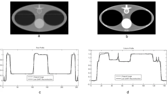
Figure 4: Line SART reconstructed images after 100 iterations using a line source of length 5 cm at two different display windows with profiles along the dotted line. a) Reconstructed image at a display window of [0, 2]. b) Reconstructed image at a display window of [0.8,1.2]. c) Profile of the row. d) Profile of the column.
a b
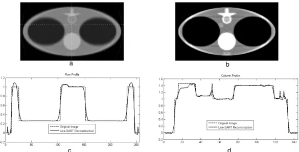
Figure 5: Line SART reconstructed images after 100 iterations using a line source of length 8 cm at two different display windows with profiles along the dotted line. a) Reconstructed image at a display window of [0, 2]. b) Reconstructed image at a display window of [0.8,1.2]. c) Profile of the row. d) Profile of the column.
a b