Local, multi-resolution detection of network communities by Markovian dynamics

Imperial College London Department of Mathematics

Local, multi-resolution detection of

network communities by

Markovian dynamics

Yun William Yu

March 2014

Supervised by Mauricio Barahona & Sophia Yaliraki

Submitted in part fulfilment of the requirements for the degree of Master of Philosophy in Mathematics of Imperial College London

Declaration

I herewith certify that all material in this dissertation which is not my own work has been properly acknowledged.

Copyright

The copyright of this thesis rests with the author and is made available under a Creative Commons Attribution Non-Commercial No Derivatives licence. Researchers are free to copy, distribute or transmit the thesis on the condition that they attribute it, that they do not use it for commercial purposes and that they do not alter, transform or build upon it. For any reuse or redistribution, researchers must make clear to others the licence terms of this work.

Acknowledgements

I would like to thank my supervisors, Sophia Yaliraki and Mauricio Bara-hona, for their immeasurable assistance through the entire process, and Jean-Charles Delvenne for insightful discussions and advice.

Also, I would like to thank all the members of both the Yaliraki and Bara-hona research groups, especially Antoine Delmotte and Michael Schaub, for useful comments and some of the example networks used.

The Imperial Marshall Scholarship, jointly funded by Her Majesty’s Gov-ernment and Imperial College, made this research possible.

Finally I would like to thank my parents for giving me the time and sup-port to finish writing this thesis.

Abstract

Complex networks are used to represent systems from many disciplines, including biology, physics, medicine, engineering and the social sciences;

Many real-world networks are organised into densely connected

communi-ties, whose composition gives some insight into the underlying network.

Most approaches for finding such communities do so by partitioning the network into disjoint subsets, at the cost of requiring global information and that nodes belong to exactly one community. In recent years, some ef-fort has been devoted towards the development of local methods, but these are either limited in resolution or ignore relevant network features such as directedness.

Here we show that introducing a dynamic process onto the network allows

us to define a community quality function severability which is inherently

multi-resolution, takes into account edge-weight and direction, can accom-modate overlapping communities and orphan nodes and crucially does not require global knowledge. Both constructive and real-world examples— drawn from fields as diverse as image segmentation, metabolic networks and word association—are used to illustrate the characteristics of this ap-proach. We envision this approach as a starting point for the future analysis of both evolving networks and networks too large to be readily analysed as a whole (e.g. the World Wide Web).

On more theoretical fronts, severability quantifies the relevance of a time scale separation of the dynamic process, allowing us to set apart the commu-nity at short times or aggregate it to a super node at large times. This also offers the potential for quantitatively exploring the underlying connections between network community detection, model reduction and diffusion-like processes.

Contents

Acknowledgements 4 1 Introduction 12 1.1 Thesis structure . . . 14 2 Literature review 16 2.1 Mathematical notation . . . 16 2.2 Hierarchical Clustering . . . 17 2.2.1 Agglomerative methods . . . 19 2.2.2 Divisive methods . . . 20 2.3 Quality functions . . . 24 2.3.1 Modularity . . . 24 2.3.2 Spin glasses . . . 25 2.3.3 Stability . . . 26 2.3.4 Information theoretic . . . 27 2.4 Local approaches . . . 28

2.4.1 Local modularity variants . . . 28

2.4.2 LFR fitness . . . 30

2.4.3 k-clique percolation . . . 31

3 Severability 33

3.1 Formal definition . . . 35

3.2 Meaning . . . 36

3.3 Relationship to existing methods in the literature . . . 38

3.4 Optimisation procedure . . . 41

3.5 Computational complexity . . . 43

4 Constructed benchmarks 45 4.1 Hierarchical random graph . . . 45

4.2 Variants of the LFR benchmark . . . 47

4.2.1 Comparison methods . . . 47

4.2.2 Unweighted, undirected, non-overlapping networks . . 50

4.2.3 Unweighted, undirected, overlapping networks . . . 52

4.2.4 Weighted, directed, overlapping networks . . . 53

4.3 Ring of rings . . . 54

4.4 Square lattice . . . 55

5 Real networks 57 5.1 Word association, overlap, & orphans . . . 57

5.2 Metabolic networks . . . 59

5.3 Image segmentation & commutativity . . . 62

6 Future Work 65 6.1 Computational optimisation . . . 65

6.1.1 Proof of concept . . . 66

6.1.2 Numerical stability . . . 68

6.1.3 Conclusion . . . 69

List of Figures

2.1 Hierarchical clustering . . . 18

3.1 Painting landscapes . . . 34

3.2 Random walk history . . . 35

3.3 Optimisation procedure . . . 42

4.1 Hierarchical random graph . . . 46

4.2 Unweighted, undirected, non-overlapping LFR benchmark . . 51

4.3 Unweighted, undirected, overlapping LFR benchmark . . . . 52

4.4 Weighted, directed, overlapping LFR benchmark . . . 53

4.5 Ring of rings . . . 54

4.6 Square lattice diffusion . . . 56

5.1 Word association . . . 58

5.2 Word association - a larger view . . . 60

5.3 Citric acid cycle . . . 61

1 Introduction

Complex networks are used to represent systems from many disciplines, in-cluding biology, physics, medicine, engineering and the social sciences [65]. In the social sciences, one of the traditional bastions of network science, networks are used to represent people and the connections between them: friendships, romantic pairings, work colleagues, etc. [54, 72, 76]. In engi-neering, electrical wiring, on both macro and micro scales, from country-wide grids [3] to the components on individual chips [33], serves as an-other historically relevant example. More recently, this abstraction has also proven revealing in biochemistry, being used for kinetic transition networks [67], interaction networks [42] and structural networks [17]. By abstract-ing away the details of connections between members of a set into possibly weighted and/or directed edges, the same mathematical methods can be used to analyse networks generally.

It is widely accepted that one of the distinguishing characteristics of com-plex networks is community structure [54], where communities (also known as partitions, modules, or clusters) are sets of nodes with stronger internal than external links. Depending on the underlying network, these commu-nities might map to groups of friends [76], genes and proteins involved in a particular function [75] or the pixels on an image representing an object [62]. Unfortunately, though intuitively appealing, there is no single

mathe-matically precise definition of a community, and a whole host of detection methods have arisen, all with their own implicit assumptions about the na-ture of communities [12, 13, 18, 32, 36, 39, 43, 45, 48, 49, 52, 56, 57, 58, 62]. Traditional approaches partition networks into disjoint sets [18, 32, 36, 45, 48, 49, 56, 57, 58, 62], which works well when nodes must belong to exactly one community, such as in the partitioning of tasks to multiple nodes in a computing cluster for parallel processing [63]. However, in real networks, nodes will often belong to multiple or even no communities [39, 52]. For example, most people have both work and family social circles; hard partitioning excludes such overlap. Conversely, while many weblogs belong to “blog rings” sharing similar interests—e.g. cooking, mathematics—there are a significant number without such affiliations.

Furthermore, communities can not only overlap but be completely em-bedded within each other: all physicists are scientists, but not all scien-tists are physicists. To detect such embeddings, resolution parameters are needed [26]. Algorithms that are combinatorial in construction, based on counting and/or cutting links [12, 13, 28, 39, 43, 45, 48, 49, 52, 56, 62] do not naturally include such resolution parameters. These have often been

added later, sometimes ad-hoc [39], sometimes through connections with

other phenomena such as spin glasses [56] or Markov chains [36, 18]. Perhaps more importantly, methods that are global in scope, including spectral [32] and information theoretic [57, 58] algorithms, also result in an unintuitive artefact: whether a set of nodes is considered a good community is dependent upon the entire network in which it is embedded. This also results in practical problems where the entirety of a network is not known, as updating the network representation with more accurate information might completely change the results.

The role of community detection has increased greatly in prominence due to the massive data acquisition and proliferation caused by a wealth of recent technological advances. Its goal should be to give insight into such large but opaque and uninformative datasets which are not enlightening on their own. It is thus imperative to resolve the outstanding problems enumerated above. Here, we propose such a method that is local, multi-resolution and allows for both overlapping and orphan nodes, as well as directed and weighted links.

1.1 Thesis structure

This work has been organised around its main result, severability. The mathematical and historical context is first provided, the result is presented, and future implications are suggested.

Chapter 2 introduces the mathematical notation necessary and surveys the history and current status of community detection methods.

Chapter 3 introduces severability, a community quality function based on results from Markov chain quasi-stationarity. Furthermore, an opti-misation procedure is presented that is well-suited for optimising local quality functions.

Chapter 4 assesses the performance of severability on appropriately chosen artifical benchmark graphs against existing popular methods.

Chapter 5 demonstrates some of the more pertinent properties of sever-ability by application to several real-world networks, including word-association, image segmentation and a biochemical network.

Chapter 6 highlights some potential areas for future work, including the search for a fast method for determining the eigenvalues of an ex-panded matrix.

2 Literature review

There are far too many variations on community detection methods in the literature to describe in detail here [60]. In this chapter, we restrict our-selves to a subset of proposed methods, comprising those that have been key

influences on the development of our methodseverability and/or popular in

the field.

2.1 Mathematical notation

Formally, a mathematical graph G is defined as a set V of nodes (or

ver-tices) together with another setE of links (or edges) between vertices. Let

n=_|V_| and m=_|E_|, the total number of nodes and vertices respectively.

Depending on the context, links can be either directed (such as hyperlinks on the web) or undirected (such as collaboration networks). Additionally, weights can be assigned to links according to a connection strength.

The topology of a graph is encoded in the adjacency matrix A, where

aij is the weight on the link from node i to node j. If there are multiple

links, letaij be the sum of their weights. Define the out-degreedi to be the

sum of the weights of all links leaving nodei. Then the out-degrees can be

compiled in the vectord=A1, where1 is the n_×1 vector of ones. Define

D= diag(d) to be the diagonal matrix of out-degrees.

chain in which the probability of leaving a node is split amongst the outgoing links proportionally according to their weights, with a transition probability aij

di for each link.

xt+1=xtD−1A≡xtP (2.1)

wherextis the 1×nnormalised probability vector andP is the transition

matrix.

LetH_∈Mn×c(R), wherecis the number of communities, be the partition

indicator matrix such that

Hij = 1 ⇐⇒ i∈Cj

Hij = 0 ⇐⇒ i6∈Cj,

whereCj ⊂V is a community. We use this notation only for hard partitions,

soCi∩Cj =∅ ⇐⇒ i6=j. As there is an isomorphism between indicator

matrices and partitions of a graph, it is possible without risk of confusion

to refer to thepartition H.

2.2 Hierarchical Clustering

One of the classical methods for finding groups in datasets is hierarchical clustering [70, 46]. A general method, hierarchical clustering requires only a dissimilarity measure between members of the set and thus is not restricted to network clustering. For networks, the dissimilarity measure is usually related to either the number of links or paths between clusters.

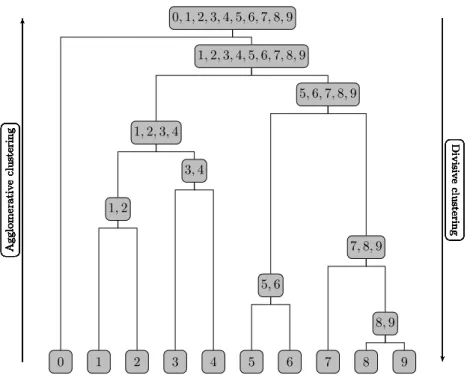
The method is based on building a dendrogram of clusters (figure 2.1). At the top is the entire graph, at the bottom the individual nodes, and in the intermediate slices, partitions consisting of clusters of varying sizes. As one

0 1 2 3 4 5 6 7 8 9 8,9 Agglomerativ e clustering Divisiv e clustering 5,6 Agglomerativ e clustering Divisiv e clustering 7,8,9 Agglomerativ e clustering Divisiv e clustering 1,2 Agglomerativ e clustering Divisiv e clustering 3,4 Agglomerativ e clustering Divisiv e clustering 1,2,3,4 Agglomerativ e clustering Divisiv e clustering 5,6,7,8,9 Agglomerativ e clustering Divisiv e clustering 1,2,3,4,5,6,7,8,9 Agglomerativ e clustering Divisiv e clustering 0,1,2,3,4,5,6,7,8,9 Agglomerativ e clustering Divisiv e clustering

Figure 2.1: Hierarchical clustering can be depicted as a dendrogram. Ag-glomerative methods work by merging together smaller clusters (going up the dendrogram), while divisive methods split larger clusters (going down the dendrogram).

goes up the dendrogram, clusters merge together; as one goes down, clusters are divided into smaller ones. These two directions also correspond with the two types of hierarchical methods used, respectively the agglomerative and divisive methods.

2.2.1 Agglomerative methods

This is a family of methods that operates by iteratively forming clusters from nearest neighbours [46]. Using the original network, weights are assigned between every pair of nodes according to a measure of how dissimilar they are. Different measures of similarity between nodes include counting the total number of node-independent paths or total number of link-independent paths [72]. Choice of the measure is dependent both on computational considerations and on the nature of the network.

Initially, each node is assigned to its own cluster. At each step, the two “nearest” clusters are merged; the process stops when all nodes are assigned to a single cluster. Because the identity of the clusters change at every step, dissimilarity must be redefined; different algorithms use various approximations to minimise the computational cost [46]. Communities are

defined as the clusters formed aftertsteps. Once nodes are grouped together

in the same cluster, they remain so for the entirety of the method, resulting in a hierarchy of communities containing all the clusters that merged to form it. Similar techniques have been used in the chemical physics literature in the form of recursive regrouping to generate dendrograms of Markov states known as disconnectivity graphs [68].

One shortcoming of hierarchical clustering is its tendency to isolate nodes on the periphery. For instance, in variations that make use of counting paths, a node that is connected by only a single link to a cluster will remain

isolated for a large number of agglomeration steps.

2.2.2 Divisive methods

Instead of iteratively merging smaller clusters together, divisive methods start with all nodes grouped together and iteratively separate them. Some-times, this is done by removing links one-by-one according to some heuristic. For instance, the edge betweenness algorithm first lists all the shortest paths between all pairs of nodes, and then removes the links which are included in the most number of shortest paths [28]. As links between communities serve as the bridges between nodes in the respective communities, a higher number of shorter paths run along them; thus, they are cut away first.

More often though, divisions are made by optimising for some global tition penalty function. For hierarchical clustering, even when using

par-tition penalty functions—which often permit k-way divisions for arbitrary

k—each step generally consists of finding only the best 2-way partition.

This has the advantage of being comparatively easy to optimise through spectral methods [61]. As penalty functions share many similarities with severability, our community quality function, we go into some detail on the construction of several graph partition penalty functions.

Minimum Cut

Possibly the simplest possible penalty function is one summing together the total weight of links cut [33]. The minimum cut

using the entry-wise matrix 1-norm. The number of clusters k must be

specifieda priori—otherwise,k= 1 trivially minimises the number of links

cut. Note that this is equivalent to finding a permutation matrix P such

thatP APT _{is almost block diagonal.}

The minimum cut criterion works well for the problem of partitioning

graphs into k clusters of at most size c, such as appears in the division of

tasks for parallel processing or the construction of circuit boards. However, in the problem of community detection, one often does not have prior knowl-edge of either the number of clusters or their respective sizes. Furthermore, this method can suffer from the same shortcoming as the agglomerative hierarchical clustering, in that it can isolate small groups nodes on the pe-riphery. This is a ready consequence of the fact that assigning small groups of peripheral nodes to a community results in fewer links being cut [73].

For large graphs, minimising the penalty function through such methods as Kernighan-Lin switches [33] can be extremely computationally intensive. However, more efficient algorithms have been developed, including a recur-sive spectral method based on solving a generalised eigenvalue problem [69], which leads to hierarchical clustering.

Ratio Cut

To resolve the issue of isolating peripheral nodes, ratio cut was proposed:

RCut(H) = cut(H)

|C1|

+cut(H)

|C2| .

whereC1, C2 are the two clusters [71]. By normalising the cutting penalty

against the size of each cluster, unbalanced partitions, wherein communities are of extremely different size, are selected against.

A spectral method for bisecting the network is offered through the lapla-cian matrix

L=D₋A.

If the eigenvector corresponding to the 2nd smallest eigenvalue of L (also

known as the Fiedler eigenvector [25]) is small, then bisecting the network according to the sign of each entry of the eigenvector will result in a small cut [1]. This provides the basis for a hierarchical partitioning using ratio cut through iterative 2-way partitions.

Normalised Cut

Another attempt to resolve the tendency of minimum cut to isolate periph-eral nodes can be achieved by normalising the cutting penalty against the total link weight from each community, rather than the community size.

This provides the basis of the normalised cut [62]. Let H be a bisection

such that HTAH =    L11 L12 L21 L22   ,

socut(H) =L12+L21.Then the normalised cut is

N Cut(H) = cut(H)

L11+L12

+ cut(H)

L21+L22

.

Although isolating small groups of peripheral nodes may cut fewer links, those links make up for a larger proportion of their total, and so the nor-malised cut penalty even more severely penalises unbalanced partitions than does ratio cut.

Normalised cut also has a spectral approximation. Each of the columns

eigenvector solutionsq of

(D₋A)q =λDq.

Note that the clusters identified are generally not exactly correct because of the relaxation necessary in transitioning to the continuous domain of real eigenvectors.

MinMax Cut

MinMax cut normalises the cutting penalty against the internal connectivity of each cluster [19]. Using the same notation as above,

M inM axCut(H) = cut(H)

L11

+cut(H)

L22

,

which can be rewritten

M inM axCut(H) = x

T_(D−A)x

xT_Ax +

yT_(D−A)y

yT_Ay .

This turns out to provide even more balanced cluster sizes than ratio or normalised cut [50].

As with normalised cut, the usual method employs spectral relaxation

and finding the generalised eigenvector solutionsq where

(D₋A)q =λDq.

Again, the solutions are not exact, and often, further refinements like k-means are needed in post-processing to find more optimal partitions; more recent modifications of MinMax cut provide better resolutions to this

prob-lem [50].

2.3 Quality functions

The distinction we draw between divisive hierarchical partition penalty func-tions and partition quality funcfunc-tions is highly artificial, lying only in the way they are applied. The penalty functions considered in the previous section are intimately tied to their respective optimisation methods, generally be-ing used for recursive bisection to generate a dendrogram of communities. On the other hand, the quality functions considered in this section are in practice more separated from the heuristics used to optimise them.

Although both are functions from the space of possible partition matrices

HtoR, the separation of optimisation procedures from quality of partition

marks an important paradigm shift. As a gross oversimplification, scientists no longer simply try to find partitions, but are more interested in evaluating how good those partitions are.

2.3.1 Modularity

One extremely popular alternative to purely cut-based approaches is mod-ularity [48]. It’s computed by taking the number of intra-community links and subtracting the expected number of intra-community links, given an appropriate model of a random graph.

More precisely, for a partition intoc communities,

modularity = 1 2m c X l=1 X i,j∈Cl Aij − kikj 2m .

takes into account the expected number of links. That is to say, in this case, the expected number of links is proportional to the degree of the node, as would be the case in a random graph (under the configuration model of a random network).

Although modularity was originally employed through recursive bisection, as in the divisive hierarchical algorithms, it eventually grew to take on a life of its own as primarily a quality function for which many varied optimi-sation methods exist [15]. Unlike hierarchical clustering, using modularity to detect communities gives only a single partition, as opposed to an entire hierarchy of partitions—this is true even when using recursive bisections, as modularity gives reason to choose one particular slice of the hierarchy over all others. Although this is not necessarily a shortcoming of the method, it does result in modularity only being able to detect communities on certain scales [26]. When the most natural community size is below the resolution scale, modularity does not give the correct answer. Furthermore, in the case of naturally hierarchical graphs, wherein communities are obviously embedded within one another, modularity can only give a single slice.

2.3.2 Spin glasses

One class of attempts to resolve the resolution scale limitations of modular-ity comes from connections to statistical physics by viewing the clustering problem as the assignment of spins in the ground state of a spin glass [4, 56]. We focus here on the Pott’s Hamiltonian of Reichardt and Bornholdt [56], given by

H(σ) =₋X i6=j

whereσis a vector specifying the spin states of each node,pij is the expected

probability of a link between nodes, and γ is a scaling factor determining

the ratio of energy that can be contributed by links vs non-links.

Minimising the energy of the system takes the place of optimising for a

quality function. Additionally, by varyingγ, one is able to recover

commu-nities at different resolutions. Furthermore, when the expected probability

of links between nodes pij = kikj/2m and the scaling factor γ = 1, it is

straight-forward to verify that the Hamiltonian becomes a constant multi-ple of modularity.

2.3.3 Stability

Stability is based on analysing the behaviour of a Markov process on the graph [18, 36]. Although theoretically, any choice of a Markov process could be used, the most natural choice is the standard random walk, with the nodes corresponding to Markov states and the probability of transition directly proportional to the weight of the out-links from nodes. Roughly, stability measures the probabilities for random walkers to remain in their starting communities.

Given the clustered auto-covariance matrix

R(t, H) =HT_(ΠMt_−πT_{π)H, (2.2)}

R(t, H)ij is the probability that a random walker originating from

commu-nity Ci will still be in Cj at time t, minus the contribution towards that

probability arising solely from the respective vertex degrees.

However, that includes the probability that a random walker will leave and later return to the community. To account for that, stability is defined

by

r(t;H) = min

0≤s≤ttrace[R(s, H)]. (2.3)

Thus formulated, Markov time plays the role of the resolution parameter, allowing for discovery of communities at multiple scales.

Although it is not entirely obvious, stability turns out to have deep con-nections with several of the clustering methods presented above. At a

Markov time t = 0, stability corresponds to normalised cut, at t = 1 to

modularity under an appropriate null model, and at t _{→ ∞} to spectral

clustering [18]. Furthermore, the linearisation of stability from 0< t < 1

happens to be equivalent to the Pott’s Hamiltonian model [36].

2.3.4 Information theoretic

Another set of approaches proposed by Rosvall and Bergstrom utilises an information-theoretic framework for community detection [57, 58, 59]. We do not go into as much detail here because they are not as closely related to severability as many of the previous methods; however, this approach has been extremely successful at certain benchmarks [40].

Infomod views partition assignment through the lenses of signal

trans-mission [57]. Say Alice has full information about a graph G and wants

to inform Bob. However, there is limited transmission bandwidth, so Alice

instead only transmits the partition and Bob tries to reconstruct G from

the partition. Infomod’s quality function measures how similar the recon-struction is to the original graph.

Infomap follows a similar scheme, but introduces random walk dynamics [58]. Alice is attempting to use a partition assignment to optimally compress the path-history of the infinite-length random walk, which is then

transmit-ted to Bob. Instead of sending the path history as a list of nodes traversed, compression is achieved by readdressing the nodes according to community assignment using a prefix/postfix pattern. Then, if a random walker moves from one node within a community to another within the same community, only the postfix needs to be transmitted. Compression is thus optimal when the inter-community hops are rare.

Furthermore, to better understand hierarchical communities, infomap can be modified to produce multilevel partition trees [59]. Instead of using the 2-level prefix/postfix pattern, even more optimal compression of a random walker’s infinite path history can often be achieved by subdividing commu-nities.

2.4 Local approaches

One of the common features of all of the partitioning methods reviewed above is the lack of overlapping communities. Although it is possible to generalise some methods to permit “fuzzy” partitions [74], most recent at-tempts instead centre around local algorithms that do not depend on global knowledge. This approach has the advantage of naturally permitting both overlapping communities and communities of extremely varying size (in-cluding “orphan” nodes).

2.4.1 Local modularity variants

Given modularity’s popularity as a community detection method, it is un-surprising that there have been many attempts to define a local variant. Let

us define for setsX_⊂Y _⊂V A(X, Y) =1 2   X i∈X X j∈Y (Aij +Aji)− X i,j∈X Aij  ,

the sum over all edges inY with at least one endpoint inX.

Now consider a community of nodesC_⊂V with boundary nodesB _⊂C.

Clauset’s local modularity measureR [13] can be defined by

R(C) = A(B, C)

A(B, V),

the ratio of the sum over edges in C with at least one endpoint in B and

the sum over all edges with at least one endpoint inB.

Similarly, Luo, et al, proposed a modularityM [43] defined by the ratio

of the sum over edges inC to the sum over edges with exactly one endpoint

inC. This can be expressed using the above notation as

M(C) = A(C, C)

A(C, V)− A(C, C),

Unsurprisingly, it can be related toR: in the special case whereC =B, the

thresholdsM ≥1 and R≥0.5 are equivalent [12].

Chen, et al, proposed a similar local community metric L [12] defined

by the ratio of the average number of neighbours each node in C has in

C to the average number of neighbours each node in B has outside of C.

Translated into a slightly different form, that is equivalent to

L(C) = 2A(C, C)/|C|

(A(B, V)− A(B, C))/|B|.

short-coming that makes them unsuitable to use as community quality functions.

Taking C to be the entire network is either always a global maximum

(though use of the extended real line is needed to make the latter two

func-tions well-defined when resulting in_∞). Much like the divisive hierarchical

partitioning algorithms (whose penalty functions were minimised when all nodes belonged to a single cluster), making use of these functions requires

specifyinga priori the expected size of a community. The optimisation

rou-tine becomes as important as the quality function, so the latter cannot be an objective metric.

Furthermore, as with modularity, none of these local variants includes a resolution parameter of any sort. Thus, even when the expected community sizes are specified, these functions are unable to adequately probe at certain scales or reveal multilevel community information.

2.4.2 LFR fitness

One attempt to add a resolution parameter to these local modularity vari-ants was proposed by Lancichinetti, et al [39] in the form of the following fitness function (using previous notation):

fC =

2_A(C, C) (A(C, V) +A(C, C))α

The α factor allows tuning the method for different size communities. For

α ≤ 1 the global maximum for the fitness function is always the entire

network, but for α > 1 that is not necessarily true (despite the original

paper claiming it to be so [39]).

However, as presented, the fitness function is still intimately connected with the optimisation procedure and is not used as true fitness function.

In their agglomeration method for finding communities, instead of trying to find the global maximum (which is in many cases the entire network), Lancichinetti, et al, instead stop the process once the first local maximum is found [39].

Furthermore, the internal structure of the community is not taken into account by the fitness function beyond summing together all the edges. This causes the unintuitive result that even disconnected sets of nodes can score high on the fitness function, which is only prevented by their particular optimisation procedure.

Lastly, althoughα mostly works as a resolution parameter, it is a purely

ad hoc construction, without any deeper theoretical justification like con-nections to Markov processes or spin glasses. For these reasons, although the motivations and ideas behind the construction of the LFR fitness func-tion were laudable, there is still much room for a better local community quality function.

2.4.3 k-clique percolation

Of course, community quality functions are not entirely necessary for a local

approach to work. k-clique percolation, as introduced by Palla and Vicsek,

is one such example [52]. Given a network,k-cliques are defined as complete

sub-graphs with k nodes. Further, define k-cliques to be adjacent if they

sharek−1 nodes. Then, a community can be defined as a set of nodes that

can be fully reached by following adjacentk-cliques [52]. This approach does

not suffer from the problem of the entire network always being the optimal solution, takes into account the internal structure of the community (as it

must) and has an obvious, easily adjustable resolution parameterk.

and/or weighted graphs, due to the very definition of a k-clique. In the case of weight, the naive approach is to use a cut-off to derive a related unweighted graph. More complex approaches define an intensity measure

for k-cliques, using some of the weight information, but still requiring a

hard cut-off, this time for intensity [51]. Similarly, a directed variant of

k-clique percolation has also been proposed [53]. Although interesting for

preserving a directionality of sorts even in the clique, it does not generalise well for weighted directed graphs.

2.5 Conclusion

As has been highlighted throughout this chapter, there are a plethora of different community detection algorithms, each with particular advantages and disadvantages. However, there exist no true community quality func-tions that are local in scope, permit discovery of communities at varying resolution scales and naturally handle link weight and directionality. It is

3 Severability

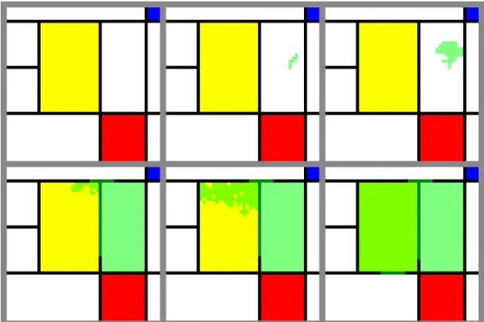
To introduce our method, we draw an analogy from energy landscapes which are often used to represent complex systems. A landscape can be imposed onto any network by introducing a dynamic process on it, for example, the standard random walk on a graph. Unlike the more familiar energy land-scapes, there is no downward arrow pointing to a minimum energy state; however, the notions of barriers and roughness translate over to communi-ties: barrier “heights” are inversely related to inter-community connection strength, while “roughness” is inversely related to intra-community con-nection strength. This is illustrated through a 3D representation of flat images, where barriers and roughness are based on differences in luminosity of adjacent pixels (figure 3.1).

We propose to define a community asseverable if it has both high barriers

and low roughness, as extracted by the behaviour of the random walkers on the underlying landscape. To do so, we borrow the concepts of mixing and retention from Markov chain quasi-stationarity [16]. Given random

walkers restricted to a communityC,C is weakly mixing if there is a strong

correlation between the walkers’ positions at Markov times 0 andt. As the

exploration ofC is also hindered by roughness, mixing is inversely related

to the roughness (see figure 3.2). On the other hand, retention is directly related to the height of the barriers, so random walkers tend to stay within

Figure 3.1: Small excerpts from Theo van Doesburg’sComposition in disso-nances (top), Paul Klee’s Ancient Sound (middle) and Claude

Monet’sthe Japanese Footbridge(bottom), their luminosity

lev-els (grayscale) and the resultant landscapes. Top and bottom are extreme cases, respectively with either obvious or nonexis-tent communities. In middle, although there is significant inter-nal roughness, slightly higher barriers exist.

Figure 3.2: The path history of one particular random walker highlighted in green. Note that the regions of solid colour (low roughness) get explored before crossing the colour-shift barriers. Thus, as is natural, the solid colour regions (except for the black borders) correspond to communities, but not any other arbitrary areas.

C if it is hard for them to escape.

3.1 Formal definition

Given a connected subsetC⊂V, we consider the behaviour of the random

walk onC. Let Qbe the sub-matrix ofP corresponding to nodes in C, and

letk=_|C_|, the size of the community. Then we define the retentionρ(Q, t),

the probability for a random walker starting with a uniform probability

distribution inC not to have escaped by time tas

ρ(Q, t) = 1

k 1

T_Qt₁

To define mixing, first let q_i(t) be the ith row of the matrix Qt_{. Because}

C is connected, q(_it) ₆= 0. Thus q

(t)

i

q(_it)1, a unit-normalised row of Q, is the

probability distribution at timet for a random walker starting from node

i, conditional upon the walker remaining in C. We can then define the

internal mixingµ(Q, t) as µ(Q, t) = 1− 1 k k X i=1 kq¯− q (t) i q_i(t)1kT V, (3.2)

where ¯q is the arithmetic mean over the unit-normalised rows of Qt_{. We}

have used the fact that the total variation distance norm is given by

δT V(v) = 1 2 X i |vi|. (3.3)

Both ρ and µ are defined to range from 0 to 1, where the a value of 1

corresponds to perfect retention or mixing, respectively. We can now define

the community quality functionseverability by

σ(Q, t) =ρ(Q, t) +µ(Q, t)

2 . (3.4)

Severability has the intrinsic resolution parameter of Markov time; as t

increases, the random walker will diffuse to larger parts of the graph.

Ad-ditionally, since it depends only upon the out-links from nodes withinC, it

is a purely local function.

3.2 Meaning

For time t, the retention of a community is a measure of the error

the network, i.e. has a zero escape probability. The internal mixing on the other hand indicates how close the distribution within the community is from the quasi stationary distribution—for instance, in the context of energy landscapes and discrete path sampling, mixing is equivalent to the

local equilibrium condition. Therefore, severability at timetis close to one

if the dynamics of the random walker starting from a node in the commu-nity are equally unaffected by aggregation of all states in the commucommu-nity for

times larger thantand disconnecting the community for times smaller than

t. Moreover, for a given community, the severability will reach a maximum

at a time which can be interpreted as the best separator between the short run and long run regimes.

This is related to the the existence of time scale separation in random walker dynamics. Given a partition of the states in a linear system, if inter-community transition probabilities are sufficiently low, then at short times, the Markov chain can be approximated by a description of its dynamics on completely disconnected communities. Conversely, because at high times the random walkers approach the quasi-stationary distribution within com-munities, the dynamics of the entire system can be accurately described as an aggregated Markov chain with every community collapsed into a single state [64, 2, 14].

Severability provides a way of quantifying the error committed in col-lapsing a set of states, without needing to know the entire system. Being a local approach allows in principle the detection of all overlapping or disjoint communities, each with their own time scale. On the other hand, the pre-vious approaches cited require a strict partition into communities, all with the same characteristic time scale. Such a uniformity has little reason to emerge naturally in large complex, heterogeneous networks, and can only

be obtained through the artificial grouping, splitting or trimming of natural communities.

3.3 Relationship to existing methods in the

literature

In some ways, severability can be thought of as a local extension of stability [18] in that both objective functions rely on considering the dynamics of random walkers on a graph. However, it should be noted that the clustered autocovariance matrix for stability only has an analogue to the retention term and does not directly invoke the idea of mixing.

Indeed, the use of retention only for community detection has before been explored. The local modularity functions explored in the literature review can be thought of as measuring retention for a single Markov step under different initial distributions and renormalisations of random walkers. Fur-ther, in an approximate sense, LFR fitness’ tuning factor also corresponds in some sense to retention at different (fractional) Markov times. As a more direct example, although not cast as a community detection method, the Markov Chain literature gives an example of a first passage time approach to create macrostates for more efficient MCMC [7], which also is equivalent to measuring retention.

However, as alluded to earlier, using only retention results in unintuitive pathological cases. First, retention-only approaches to creating a quality function will of necessity give a perfect score to considering the entire net-work as a community. Obviously, random walkers cannot escape from the network by definition. Thus, in all of the retention only local methods, a size limitation in the optimisation method is specified to prevent returning

the entire network as an/the optimal community. For stability, this is not a problem because the stationary distribution is subtracted out. Second, retention-only approaches do not see internal structure. If a community is disconnected from the rest of the network, it will have perfect retention even if it is itself not connected. Although in the extreme, this pathological case tends to be avoided by the choice of optimisation procedure, this means that the objective function can not be relied upon without tying it to the optimisation. Furthermore, in almost pathological cases, perhaps a commu-nity consisting of two large cliques connected by a single link, retention-only approaches will not (as intuition suggests) favour the individual cliques over the combined double clique. Global approaches like stability avoid this be-cause the entire network must be considered as a whole, and breaking up a two-clique community is favoured by the subtraction of the stationary distribution.

It is in order to avoid the problems of the previous paragraph that mix-ing must be introduced. Requirmix-ing the convergence to the quasi-stationary distribution has been implicitly used before, also in the Markov Chain lit-erature in the form of lumping analysis [41]. Indeed, the distance from the quasi-stationary distribution is exactly a measure of how accurately a single macrostate can be used to replace a collection of other states in a Markov chain. However, the method of Lempesis, et al. method operates on the entire network and measures the accuracy of the lumping at a global level. We are able to resolve this issue locally by our variance-like mixing term, which uses both “local in time” and “local in space” information from the transition submatrix power.

Another connection was hinted at previously in the analogy drawn to energy landscapes. Previous work has shown that for protein folding,

tech-niques such as transition path sampling can be used to generate a Markov chain of low-energy states connected by high-energy transition states [24, 9, 10, 11, 66]. Since in such systems, each state is associated with an actual energy level, and transitions that decrease energy level are favoured, one clever way of partitioning the state space into potential wells is to look at the disconnectivity graph. For any particular energy threshold, low-energy states are connected if the transition states between them (the barrier be-tween them) have energy below that threshold, creating a rapidly mixing community of states. Indeed, here, energy plays the same role as time in severability, whereby the communities found by the disconnectivity graph are exactly those that rapidly interconvert with low probability of jumping to disconnected states for which the barriers are too high. In this way, both retention and mixing are captured by energy.

However, although we use the language of energy landscapes to motivate the definition of severability, it is crucial to clarify that there is no require-ment for networks to correspond to actual energy landscapes. It is for this reason that instead of looking at energies, we instead look directly to the dynamic behaviour of random walkers on the graph. By directly measuring mixing and retention of random walkers, we are able to probe the same sorts of phenomenon in the more general case, at a cost of some additional complexity. Even when actual energy landscapes are involved, severability can still be applied since all it requires is the transition submatrix. Indeed, should the transition matrix be given for states on an energy landscape, severability of a community can be computed without severability having to “know” that the system is indeed an energy landscape.

A more subtle difference has to do with the nature of severability’s locality. Although the disconnectivity graph can be almost completely charactised

by the energy levels of the states and transition states between them, which allows for local determinations of energy wells, it still assumes the global structure of an energy landscape. This shows itself in the disconnectivity graph being a proper partition at any level and exhibiting the structure of a dendrogram. As we will later see, severability permits overlapping commu-nities, whereas disconnectivity graphs do not. In the application of protein transition pathways, we probably do not want overlapping communities, so severability is slightly worse in that setting; however, in many other set-tings, it is natural to think of communities overlapping, making methods like severability more applicable.

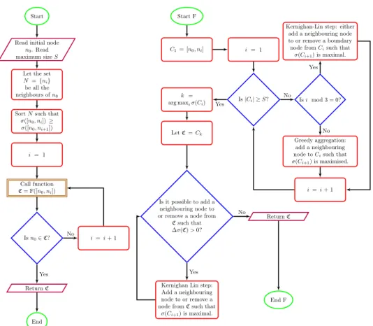
3.4 Optimisation procedure

We apply a semi-greedy search algorithm to find the optimal communityC

for a starting noden0, at a chosen Markov timetand search sizeS(see figure

3.3). Without loss of generality, defineσ(C) =σ(Q, t). Initially, only n0 ∈

C. Aggregate nodes greedily, except let every third step be a Kernighan-Lin

switch of a single node on the boundary ofC to maximiseσ(C) [33]. After

the initial semi-greedy optimisation, the intermediate communityCthat has

maximal severability is fine-tuned using Kernighan-Lin switches to find a

local maximum. If n0 is in the resulting community, then done; otherwise,

start over, but choose a neighbour that was not chosen previously for the

first step. If all neighbours of n0 have been attempted without success,

Start

Read initial node n0. Read

maximum sizeS

Let the set N={ni}

be all the neighbours ofn0

SortNsuch that σ([n0, ni])≥ σ([n0, ni+1]) i = 1 Call function C= F([n0, ni]) Isn0∈C? i=i+ 1 ReturnC End No Yes Start F C1= [n0, ni] i = 1 Is|Ci| ≥S? Isi mod 3 = 0? Kernighan-Lin step: either

add a neighbouring node to or remove a boundary node fromCisuch that σ(Ci+1) is maximal.

Greedy aggregation: add a neighbouring node toCisuch that σ(Ci+1) is maximised.

i=i+ 1 k =

arg maxiσ(Ci)

LetC=Ck

Is it possible to add a neighbouring node to or remove a node from

Csuch that ∆σ(C)>0?

Kernighan Lin step: Add a neighbouring node to or remove a node fromCsuch that

σ(Ci+1) is maximal. ReturnC End F No Yes No Yes Yes No

Figure 3.3: Flowchart of the optimisation procedure for finding the most severable community to which a node belongs. Note that in the

3.5 Computational complexity

Letnbe the number of nodes in a graph. The severability of a community

C of size k for a Markov time t can be computed in P(k, t) =O(k3_log

2t)

time, where the cubic term comes from schoolbook matrix multiplication.

Computation of mixing and retention givenQt _{are both O(k}2_{) operations,}

so the total cost is dominated by matrix exponentiation.

The cost can be reduced using fast matrix multiplications techniques;

e.g., using Strassen’s method, the total cost would only be O(k2.807_log

2t).

Alternately, for larget, matrix diagonalisation can be first employed, which

makes the t term negligible, giving a O(k3) solution, but with additional

lower-order cost. As this paper was largely a proof of principle, we have not fully explored computational optimisation.

However, finding good communities is more involved than simply comput-ing the severability of a scomput-ingle set of nodes. The community optimisation algorithm described in figure 3.3 is also costly, and more difficult to char-acterise, as it depends strongly on the number of nodes neighbouring the putative community throughout the procedure. In pathological cases, cost

isO(nM·P(M, t)), whereM is the maximum number of nodes permitted in

the community. Luckily, this upper bound only occurs in complete graphs and is largely irrelevant as most real networks are far sparser. However,

by specifyingM, one can choose the maximal computational resources one

wants to spend trying to find a community.

As before, this procedure has not been optimised for time, and there are several obvious ways of reducing cost. Besides the computation of sever-ability itself, the primary contributor to the cost is that all “neighbouring” communities’ severabilities are checked as part of the aggregation process

and subsequent Kernighan-Lin switches. A smarter algorithm could perhaps use a random walk to highlight likely candidate neighbours; for instance,

by choosing only thelnodes that a random walker uniformly distributed in

C would most likely walk to in the next step, or for removal of nodes, the

l nodes in C that have the least density of probability. Such an algorithm

would only costO(M ·P(M, t)), a significant improvement.

More subtly, the computational cost of the matrix powers might also be

reduced, by taking advantage of the fact thatQ(C∗) for each of the

neigh-bouring communities is effectively a rank-2 perturbation ofQ(C).

Further-more, as briefly mentioned in the discussion, severability is only one way of quantifying the mixing and retention of random walkers. Other alter-nate methods may be found that are quicker, perhaps using Monte Carlo simulations and the like.

4 Constructed benchmarks

To illustrate this mathematical formulation, we first apply severability to constructed benchmarks with known, pre-seeded community structure. Nat-urally, it is unavoidable that every benchmark comes with its own set of im-plicit definitions about the definition of a community. A community detec-tion method whose design follows the same definidetec-tion, whether intendetec-tionally or not, will generally perform best on that particular benchmark.

Thus, it is important to evaluate not only how well a community detection method performs on a benchmark, but whether that benchmark matches our intuition of what a community ought to be. We have attempted to use a range of very different benchmarks, but it is important to note that because the implicit definition of a community can vary, it is highly unlikely that one single method will be optimal for every problem.

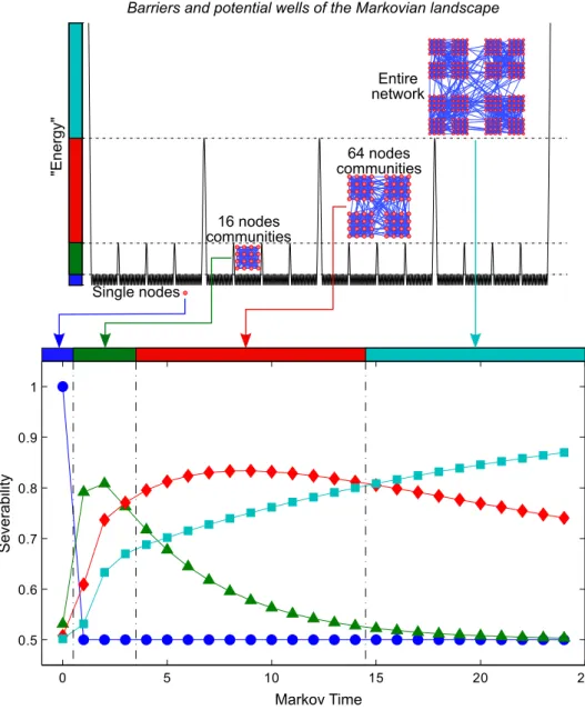
4.1 Hierarchical random graph

We optimise for severability on a hierarchical random graph with 256 nodes. Level 1 (L1) communities are composed of 16 nodes each, level 2 (L2) com-munities contain 64 nodes (four L1 comcom-munities) while the entire graph (L3) is made up of four L2 communities. The probabilities that pairs of nodes are connected when they are in the same level 1, 2, or 3 community, but

64 nodes communities Entire network Single nodes 16 nodes communities S ev er ab ility Markov Time 0 5 10 15 20 25 0.5 0.6 0.7 0.8 0.9 1 "E ner gy"

Barriers and potential wells of the Markovian landscape

Figure 4.1: The “Markovian” energy landscape of a hierarchical random graph with multi-level communities of sizes 16, 64 and 256. Sev-erability gives optimal community sizes as a function of time. Depicted are the severabilities of a single node (blue circles), 16-node community (green triangles), 64-node community (red diamond) and the entire network (cyan square).

p3 = 0.036 respectively, resulting in an average degree< k >= 16.

Varia-tions on the exact probabilities and number of levels are of course possible, but we chose here a single representative network for illustration purposes only.

This benchmark serves to illustrate the use of Markov time as a reso-lution parameter for networks with multi-level structure. As Markov time increases, the random walkers gain sufficient probability to overcome “en-ergy barriers” and hence diffuse to larger portions of the network so that the optimal community grows from single nodes to the entire network, passing through each of the intermediate levels (figure 3.1). For smaller times, it makes sense that the lower-level structure (the L1 communities) would be recovered, whereas later on, larger super-structures dominate.

4.2 Variants of the LFR benchmark

However, many real-world networks do not have such a simple distribution of community sizes. In order to provide an alternative to the Girvan-Newman model of identically sized communities [28], Lancichinetti, Fortunato and Radicchi recently proposed several new classes of benchmarks, in which the community size and node degree follow power-law distributions [40]. Addi-tionally, these benchmarks also allow for overlapping, directed and weighted networks [37].

4.2.1 Comparison methods

Optimal community cover

To compare against benchmarks which permit overlapping communities, it is necessary to generate a list of communities to cover the network. Simply

taking the optimal communities of each node is suboptimal, because then there are many duplicate communities in the list. Instead, we chose the following naive method: cover the network by communities, starting com-munity optimisations only from unassigned nodes that are on average more connected to other unassigned nodes than to previously found communities. More elaborate schemes for generating covers of a network by communities are of course possible and may indeed give better results. However, this method has the advantage of reducing the computational time required, as well as being simple to implement.

Optimal partition

To compare severability with other partitioning methods, it is necessary to turn the optimal community cover into a (hard) partition. To do so, first order the communities of the cover arbitrarily; we used the order in which the optimal community cover found the communities. Assign each node to the first community it appears in. This procedure is obviously dependent upon the ordering of the communities. In other settings, it may behoove the practitioner to develop a smarter way of assigning nodes to communities. However, in networks with well-defined partition structure, this method works sufficiently well, as will be demonstrated in analysis of the LFR benchmark graphs.

Choice of Markov Time

For hierarchical networks, Markov time serves as a useful resolution param-eter, allowing for severability to pick out optimal community structure at different levels. However, existing metrics [15, 39] require the selection of

finding optimal community covers, which is a problem common to many algorithms with resolution parameters. However, for optimal partitioning, this can be done by choosing a Markov time to minimise the total number of orphan and overlapping nodes.

Quantifying similarity

For quantifying similarity, we have employed normalised mutual information [27, 15, 35]. Coming from information theory, this metric takes the form

Inorm(X:Y) =

H(X) +H(Y)−H(X, Y)

(H(X) +H(Y))/2 ,

whereH(X) is the entropy of a random variableX andH(X, Y) represents

the joint entropy. Thus, normalised mutual information is a measure of

the shared information between the two random variablesX, Y, normalised

against the sum of their respective entropies.

In comparing partitions, the partitions take the place of the random vari-ables, and the frequency of shared nodes is used as an approximation of

probability. Let X, Y be partitions, and let cX, cY be the number of

com-munities in each partition respectively. Define a cX ×cY confusion matrix

N, whereNij is the number of nodes in the ith community of X that are

also in thejth community ofY. LetNi∗=P_jcY₌₁Nij andN∗j =

PcX

n=1Nij. Then the normalised mutual information is given by

Inorm(X:Y) = −2PcX i=1 PcY j=1Nijlog(NijN/Ni∗N∗j) PcX i=1Ni∗log(Ni∗/N) +P_jcY₌₁N∗jlog(N∗j/N) .

For comparing community covers, a generalisation of normalised mutual information that allows for overlapping nodes has been used [39]. This

communities within a partition.

We refer to the generalised variant as simply “normalised mutual infor-mation” without loss of precision as only the generalised variant can be used in the benchmarks with overlapping communities.

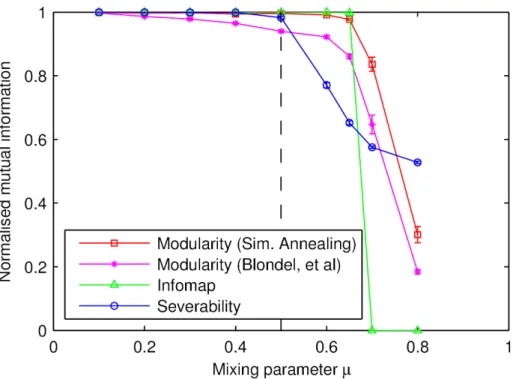
4.2.2 Unweighted, undirected, non-overlapping networks Here is highlighted the analysis of a class of networks in which communities are extremely unevenly sized, a situation in which many popular partition quality functions perform sub-optimally. These multi-scale graphs are ran-domly constructed such that both degree and community size distributions

follow power laws, with exponentsγ andβ, respectively. Additional

param-eters include the total number of nodes N, the average degree < deg >,

the maximum degreedegmax, and the mixing parameter µ- not to be

con-fused with the mixing component of severability. The fraction of links from

a node to other nodes within the same community is given by 1₋µ [40].

Graph generation parameters were chosen at values matching those in paper

of Lancichinetti et al. [40]: γ = 2, β = 2, N = 1000, < deg >= 15 and

degmax = 50. Severability optimisation was performed with a maximum

search size S = 50, and partitions were generated from the community

cover.

As can be seen from the figure, severability performs well, always

find-ing the natural community structure up to until around µ = 0.5, when

communities are no longer defined in a strong sense [55]. That severability

begins failing atµ= 0.5 is expected, since at that point random walkers are

as likely to escape during each step as to remain within any of pre-seeded communities. Recalling the definition, a community is defined as severable precisely when random walkers tend to stay and mix within it. Even so,

Figure 4.2: Comparison of severability with modularity and infomap the

LFR benchmarks with exponents γ = 2, β = 2, average degree

< deg >= 20 and maximum community size of 50. Severability

optimisation was performed with maximum search size of 50 and

Markov timet= 3 (a value determined as a result of minimising

the number of orphan nodes and overlapping nodes). Modularity was optimised for using both simulated annealing [29], which is extremely slow but gives good results, and a faster heuristic by Blondel, et al [5]. Each point is an average over ten random realisations.

Fraction of Overlapping Nodes

Normalised mutual information

0 0.1 0.2 0.3 0.4 0.5 0 0.2 0.4 0.6 0.8 1 µ t = 0.1 0 0.1 0.2 0.3 0.4 0.5 0 0.2 0.4 0.6 0.8 1 µ t = 0.3 N=1000 s min=10 s max=50 0 0.1 0.2 0.3 0.4 0.5 0 0.2 0.4 0.6 0.8 1 µ_t = 0.1 0 0.1 0.2 0.3 0.4 0.5 0 0.2 0.4 0.6 0.8 1 µ_t = 0.3 N=1000 s min=20 s max=100

Figure 4.3: Severability at Markov time t = 4, with an unweighted,

undi-rected, overlapping variant of the LF Benchmark [37]. The

net-works have 1000 nodes; the other parameters areτ1 = 2,τ2= 1,

< deg >= 20, degmax = 50. Each point is an average over five

random realisations.

the results are comparable to that of Infomap and modularity optimisation using simulated annealing, which have been found to be amongst the most successful methods for this benchmark [38].

4.2.3 Unweighted, undirected, overlapping networks

Further extensions to the LFR benchmark were made to allow for com-munities to overlap [37]. In figure 4.3, we compare the community covers from severability to the pre-seeded communities. For the optimisation, the

maximum search sizeS= 50,100 was used for the upper and lower panels,

Fraction of Overlapping Nodes Normalised mutual information 0 0.1 0.2 0.3 0.4 0.5

0 0.2 0.4 0.6 0.8 1 µ t = 0.1 0 0.1 0.2 0.3 0.4 0.5 0 0.2 0.4 0.6 0.8 1 µ t = 0.3

Figure 4.4: Severability at Markov time t = 4, with a weighted, directed,

overlapping variant of the LF Benchmark [37]. The networks

have 1000 nodes; the other parameters are τ1 = 2, τ2 = 1,

µw = 0.2, < deg >= 20, degmax = 50, smin = 20, smax = 100.

Each point is an average over five random realisations.

The parameters chosen were identical to those used for the evaluation of k-clique percolation [52] in figure 6 of Lancichinetti and Fortunato, 2009 [38]. Comparison with those results will show that severability performs comparably to slightly worse for the smaller community sizes, but signifi-cantly better for larger communities.

4.2.4 Weighted, directed, overlapping networks

Furthermore, severability also loses no accuracy when direction and weight are added to the benchmark [37] (figure 4.4). This is expected, since the Markov chain formulation naturally includes both without any modifica-tions to either the optimisation procedure or the quality function. For the

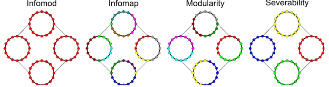
Modularity Severability Infomod Infomap

Figure 4.5: Ring of rings. Heavy lines (within rings) correspond to undi-rected links with weight 2, while light lines between rings to links with weight 1. Only severability is able to recover the

seeded ring structure (at Markov times 3≤t <10).

4.3 Ring of rings

Most constructed benchmarks [28, 40], including the ones we analysed above, base their communities on a very high density of links, modelled by cliques or random high density edge selection from a clique. Similarly, most commu-nity detection methods also adhere to this assumption; some, like k-clique percolation, make this an explicit requirement [52], whereas others like mod-ularity have null models that implicitly lead to favouring cliques.

Cliques are of course a key feature of many real world networks that severability is able to handle, as demonstrated by performance on the LFR benchmarks. However, it is instructive to examine other possibilities for community structure, since they may turn up to be of importance in man-made networks, which often have very non-random placement of links. As an illustration, consider here a collection of rings, in which a network of 64 nodes is divided into 16-node rings, with strong intra-ring links of weight 2 and weak links of weight 1 between rings (figure 4.5). Modularity (using simulated annealing [29]) and infomap [58] fail to find the most natural communities, while infomod [57] finds only the trivial community of the entire graph. Because severability is based on the retention and mixing of

random walkers, it performs considerably better; at a Markov time 3_≤t < 10, severability recovers the rings as the optimal community cover.

4.4 Square lattice

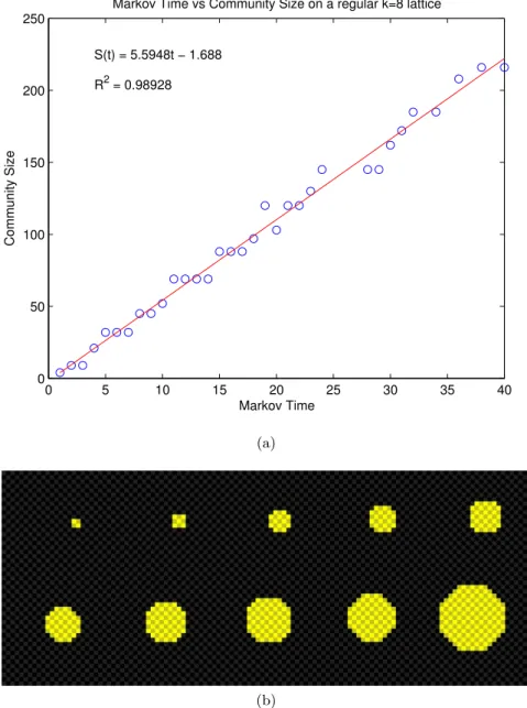
As a negative control, It is instructive to consider a network in which there is clearly no community structure. For that, we chose a regular 2-D square lat-tice with each node connected to all 8 neighbours (including diagonal links). We visualise this using a uniformly coloured discrete image, in which each pixel is connected to all of the adjacent pixels with links of equal strength. As can be seen in figure 4.6, after accounting for symmetry considerations, all communities found are transients, which is the expected result.

Additionally, these images strongly suggest a relationship between sev-erability optimisation and diffusion. This is of course quite closely related both to the dependance of severability on random walk dynamics and to the optimisation procedure outlined in 3.3. Along these lines, the optimisa-tion procedure we outlined can be thought of as a modified random walk in which previously explored states are immediately accessible to the random walker, but probability barriers in the “energy landscape” are magnified.

0 5 10 15 20 25 30 35 40 0 50 100 150 200 250

Markov Time vs Community Size on a regular k=8 lattice

Markov Time Community Size S(t) = 5.5948t − 1.688 R2 = 0.98928 (a) (b)

Figure 4.6: (a) Correlation of Markov time with size on an square lattice. (b) The transient communities found by severability on a regular lattice at Markov times t=_{1,2,3,5,8,10,11,15,18,32_}. Each block is connected to all eight of its neighbouring blocks by a single undirected edge of weight 1.

5 Real networks

It is (tautologically) always possible to construct artificial benchmarks ar-bitrarily, but only when they approximate real-world networks do they be-come relevant. In this chapter, we give examples of real-world networks that exhibit overlapping communities, orphan nodes, ring-like structure and lat-tices. Additionally, we highlight one of the key advantages of local methods, that they can be effectively used on partial graphs.

5.1 Word association, overlap, & orphans

One important aspect of community detection is the possibility of overlap-ping communities or orphans nodes. To illustrate this, we turn to a word association network that was among the examples used to highlight over-lapping communities in the introduction of k-clique clustering [52], namely the University of South Florida Free Association Norms dataset [47]. Re-searchers at the University of South Florida presented vocabulary words to study participants, who were then asked for the first word that came to mind. In constructing this network, each node corresponds to a single word, and directed links between nodes are weighted according to the proportion of responses linking those two words. For example, when cued with “sci-ence”, 21.4% of participants wrote “biology”. Thus, there exists a directed

ACORN EARTH WILDERNESS AIR JUNGLE PLANET WOODS SHADE ENVIRONMENT ENJOY LONG CLIMB LOVE BARK OAK STUMP ANIMALS RESPIRATION HIKE TREES GREEN TIMBER TRUNK DEAD LIVE LIMB BRANCH OUTSIDE HEALTH LIFE BREATH RUN EXERCISE LEAVES MAGAZINE CRAWL MOVE TRAIL IMPORTANT WALK BUSH LEG LEAF TIME DEATH ELM PINE REAL FEET JOG NATURE TREE FOREST "OAK" "WALK" "LIFE" "JUNGLE" "ENVIRONMENT" "SCIENCE" "HOME" "DELICATE" "ROSE" "MAKE UP" "ATTRACTIVE" "QUIET" "SHOW" "REACTION" "STORM" "MOUNTAIN" "HUMAN" "WHITE" "LAZY" BIRDS CLIMB HIKE CHEMICAL PRETTY VASEFLOWER CAMPING OUTDOORS TREE NATURE FOREST b a

Figure 5.1: (a) The five communities that the word “nature” belongs to. For the word association network, every neighbour of “nature” was attempted for the first step, giving the overlapping communi-ties. Nodes and links are coloured by community identification; coloured ovals represent multiple community membership. (b) A broader view of the community landscape surrounding “na-ture”, depicting also communities connected to, but not contain-ing, “nature”, including three orphan nodes. Nodes belonging to just one of the communities are combined into a single block labelled by the most central word of the community, while nodes belonging to more than one community are separately mentioned in the grey ovals. Note that in many cases, the words used to “tag” the community blocks themselves have multiple “tags”. Communities were found by optimising severability for Markov

Because cliques are only well-defined on unweighted, undirected networks, using them directly requires thresholding by weight and ignoring direction, which already discards quite a bit of information. Markov chains do not require such false dichotomies, so severability naturally admits both link direction and weight. Additionally, as a local method, it is not necessary to analyse the entire graph to find communities. Rather, by analysing more and more of the network, an ever-expanding view presents itself; figure 5.1 shows in part (a) “nature” and the communities it belongs to, while part (b) depicts the communities and orphan nodes (which are simply communities of size 1) “nature” is directly linked to (see figure 5.2).

For this analysis, we limited the maximum sizes of the communities con-sidered. However, another advantage of the method is that this in itself does not limit its applicability. This is made possible by inherent checks in the method. For example, when the maximum community size (i.e. the number of nodes) is chosen to be too small, nearly all the resulting communities will be truncated at the limit, while too large of a choice is not an issue because the Markov time itself limits the community size. Indeed, in some cases where prior knowledge of the network structure is given, artificially limiting the maximum community size can be beneficial.

5.2 Metabolic networks

A real-world example of ring structure can be found in the basic biochem-istry of the citric acid cycle. To construct the network from the citrate pathway schematic (map00020) in the KEGG database [31], each compound was used as a node, and if there exists a reaction with A as a substrate and B a product, a directed, unweighted link from A to B was assigned.