No. 2003–47
ON REPRESENTATIVE TRUST
By Charles Bellemare, Sabine Kröger
April 2003
On Representative Trust
∗
Charles Bellemare
Tilburg University, CentER, The Netherlands
{
[email protected]
}
Sabine Kr¨oger
Humboldt Universit¨at zu Berlin, Germany
{
[email protected]
}
April 30, 2003
Abstract
Because of its relation to economic growth, there is a policy interest in mea-suring social capital and average trust as its currently most important proxy. In this paper we measure societal trust and trustworthiness by combining the virtues of laboratory experiments and survey data and present results from an economic experiment conducted using a representative sample of the Dutch population. By combining both types of data, we are able investigate the determinants of trust and trustworthiness at the population level, to contrast the inferences which can be made on trust propensity using stated and revealed measures, and to test for self-selection bias through voluntary participation in the experiment.
Our results can briefly be summarized as follows. Contrary to existing laboratory based experiments, we find that stated trust measures correlate with experimen-tal trust. The effect of education and religion is shown to be depend enormously on the trust measure used. We find that the age and education profiles of ex-perimental trust are the complete opposite of those of trustworthiness, which contrast with the findings of the social capital literature. Finally, we do not find evidence of a participation selectivity bias, which is a serious concern for laboratory experiments which rely almost exclusively on volunteer participants.
∗Financial support from CentER and CentERdata is gratefully acknowledged. We thank Hanneke Dam, Marcel Das and Corrie Vis of CentERdata for their support throughout the experiment. We are grateful to Oliver Kirchkamp and Arthur van Soest for helpful discussions. Useful comments were made by participants at the NAKE Research Day in Amsterdam, the ENDEAR Workshop in Jena, the ESA European Meeting in Strasbourg, the Max-Planck-Institute in Jena, the CIRANO in Montr´eal, the DIW in Berlin, the ENTER Jamboree 2003 meeting and the Social Capital Workshop in Tilburg, the Spring Meeting of Young Economists in Leuven, and the Economics seminar in Maastricht. The second author gratefully acknowledges financial support by the Deutsche Forschungsgemeinschaft through Sonderforschungsbereich 373, Humboldt Universit¨at zu Berlin, and the EU-TMR ENDEAR Network grant (FMRX-CT98-0238). The usual disclaimer applies.
Introduction
It is increasingly argued that a nation’s social capital can influence its economic per-formance. Although there is an ongoing debate over what constitutes social capital (Bowles and Gintis, 2002, Durlauf, 2002), there seems to be a consensus that both average societal trust and trustworthiness are two important components. The trans-actions cost paradigm remains the traditional way of thinking about the mechanism by which average trust affects economic performance as higher average societal trust leads to lower transactions costs which in turn improve both the functioning of organizations and governments which ultimately leads to better economic performance.
The research on social capital started with the influential work of Putnam (1993) who found a strong correlation between measures of civic engagement and government quality across regions in Italy. The association of social capital with growth started with the work of Knack and Keefer (1997) and Zak and Knack (2001) who both find that a one-standard deviation increase in the World-Value Survey (WVS) trust index increases economic growth by more than one-half of a standard deviation. La Porta et al. (1997) find that across countries, a one-standard deviation increase in the same measure of trust increases judicial efficiency by 0.7 of a standard deviation and reduces government corruption by 0.3 of a standard deviation. The WVS trust index on which these empirical facts rests is constructed by first drawing a random sample of participants who are asked to answer a series of questions. The wording of the trust question is
WVS trust question Generally speaking would you say that most people can be trusted or that you cannot be too careful in dealing with people?
1.) Most people can be trusted. 2.) You have to be very careful. 3.) I do not know.
The WVS reports for each country the percentage of responders who indicated that ”Most people can be trusted”.
Social scientists have argued that and individuals trust will be a function of his or her past experiences (Hardin 1996). These in turn may be affected by the individuals
age, education experience with trust. It becomes relevant for policymakers to correctly measure average trust and trustworthiness and to understand how they correlate with these characteristics for two reasons. First, simply because of the strong correlation between trust, economic growth and organizational performance. Secondly, it is well known that the age and income distributions of many Western societies evolve over time in very alarming ways (Gruber and Wise, 2001). How these structural changes translate into changes in social capital levels is still not well understood but deserves investigation.
Therefore, measuring the evolution of average trust and trustworthiness in a so-ciety requires a micro level analysis. There is very little empirical evidence on the determinants of trust and most of it relies on stated trust responses from WVS type questions. Allesina and La Ferrara (2002) use data on a sample of individuals in the United-States who have answered the WVS trust question. Their empirical results show that recent history of traumatic experiences, belonging to a group which histor-ically felt discriminated and low levels of income and education have strong negative influences on trust. One drawback of this study is that it is based on the self-reported measure of trust which may be misreported by the individuals. This is particularly important since misreporting of a discrete dependent variable may lead to severely biased slope parameters even when the model correctly specifies the true unobserved categorical variable (see Bound et al., 2001, for a survey on the impact of this type of measurement error). Even though it is intuitively clear that self-reported answers to the WVS trust question may well be misreported, the empirical evidence suggesting that this is the case is scarce (see Bellemare and Kr¨oger, 2003, for a first attempt to analyze the importance of misreporting in the WVS trust question).
Economic experiments, which collect data on revealed rather than stated prefer-ences, is a potential alternative to survey trust measures. The seminal experiment of Berg, Dickhaut and McCabe (1995) (hereafter BDM) initiated an important follow-up literature and remains today the main experimental design used to assess the presence of trust and trustworthiness in a group of subjects. The BDM game is tailored to capture trust as defined by Coleman (1990) who defines an interaction as one involving trust when three contextual elements are present. i) a personS must place confidence
in the action of another person R which could lead S to experience a loss of welfare. ii) A trustworthy R behaves such that S is better (or at least not worse) off than he was before placing trust in R, iii) successful use of trust in transactions should make bothS andR better off. The BDM design captures all three components of Coleman’s definition. Numerous studies1 have extended the BDM design to asses the robustness
of the findings to different institutional and design settings.
Both survey and laboratory trust measures have important limitations. Laboratory experiments analyze behavior of subjects interacting with other participants in a con-trolled environment where decisions have real monetary consequences. This method has the virtue of measuring revealed trust intentions of individuals at the expense of generally doing so with homogenous student subject pools lacking the required varia-tion in background characteristics to measure the parameters of interest. On the other hand, survey data like the World Value Survey observe responses in hypothetical situa-tions from an heterogenous sample of a population at the expense of measuring stated preferences for trust.
The analysis of the determinants of trustworthiness is even less documented than trust, in part because there does not exists any satisfactory survey question which seems to embody the distinctive features of trustworthiness. Our current empirical knowledge has been provided by laboratory results which analyze responders behavior in trust games, the most famous of being the BDM game2. Overall, these studies have
shown that trustworthiness, like trust, is robust to different institutional settings and designs (see the above references). Once again, the lack of heterogeneity in the subject pool prevents population inferences and complete measurement of its determinants. To our knowledge, there does not exists any micro level analysis of the determinants of trustworthiness in a society. This is troublesome as recent research has shown that 1Glaeser et al. (2000) measure social capital among participants with the BDM game and
addi-tionally by analyzing the willingness to pay in a dropped envelope game. Gneezy, G¨uth, and Verboven (2001) investigate whether distributional considerations might explain the trustor’s behavior by vary-ing the range from which the trustee can send back. Burks, Carpenter, and Verhoogen (2003) study whether changing roles in a trust game gives rise to a more cooperative outcome as both parties experience all situations as trustor and trustee. Ortmann, Fitzgerald and Boeing (2000) find that the results of BDM are quite robust using different frames. All these papers find that the results of the BDM experiment are robust and lead to conclude that revealed trust is an important aspect of economic behavior.
trustworthiness could be ”the” economically relevant component of social capital to understand the process of economic development (Francois and Zabojnik, 2002). If this were the case, then the lack of empirical evidence on the determinants of average societal trustworthiness is source of concern.
This paper makes two important contributions. First, we add to the scarce body of knowledge on the determinants of trust and measure age, education and other life experience effects of experimental trust responses from the BDM game. We do so by having a random sample of the Dutch population play a computerized version of the BDM game. A side product of our analysis is that we are able to contrast the inferences which can be achieved by using stated and revealed trust preferences. To do so, we propose a new minimum distance test statistic based on the distance between the underlying data generating processes of the stated and the revealed trust responses. Our evidence shows that the effect of some background characteristics can change dramatically when using the stated rather than the experimental trust responses.
Secondly, we shed a first look into the determinants of trustworthiness in a popu-lation. We follow the established trend of analyzing the choices of subjects assigned to the role of respondents in the BDM game. The crucial difference between our study and the existing literature is the heterogeneity of the responders background charac-teristics. To our knowledge, this is the first empirical assessment of the determinants of trustworthiness at the society level. We find that the education and age patterns to be the complete opposite of those of trust.
The paper makes some additional contributions. First, we depart from most trust experiments and elicit subjects’ beliefs about their partner’s action. We find that subjects’ beliefs play a fundamental role in determining both trust and trustworthiness behavior.
Secondly, our paper allows to asses whether the inferences made using a random sample of the population differ substantively from those one could make using the more traditional student subject pools. The idea of using more heterogeneous subject pools in experimental economics is not new as testing the assumption of ”parallelism” between the lab and the field has been a source pre-occupation for some time. The most popular mediums to reach more diversified participants have been newspaper
ex-periments (e.g. Bosch-Dom`enech et al., 2002, G¨uth, Schmidt and Sutter, 2002), and, more recently, the Internet (e.g. Lucking-Reiley, 1999). These papers generally find that newspaper and lab subjects have similar unconditional behavioral responses. One drawback of these studies is that one cannot make inferences on societies’ average be-havior as the subjects are not drawn randomly from the population of interest. Two noteworthy experiments have recently been run with representative samples. Harrison et al. (2002) setup an laboratory experiment to investigate the heterogeneity in indi-vidual discount rates. Their sample consists of a small random sample of the Danish population. Hey (2002) used a random sample of the Dutch population headed by the CentERpanel of Tilburg University and had them play an experiment on decision making under risk and uncertainty.
Thirdly, an inevitable consequence of most laboratory experiments is that they can-not control for the fact that subjects with specific unobserved characteristics such as high gambling predispositions and low risk-aversion self-select themselves to partici-pate in the experiment. If these unobservable factors are related to the outcome that is measured in the lab, a familiar selection bias will be present (Heckman, 1978, 1990). Eckel and Grossman (2000) have attempted to investigate participation bias in lab-oratory experiments. Comparing student volunteers to student non-volunteers3 they
conclude that volunteers perform significantly differently. By giving our subjects the choice to participate in our experiment and by observing the characteristics of those who refuse to do so, we are in the unique position to test for participation bias in our experiment and control for its effect.
The remainder of the paper is organized as follows. Section 1 describes the de-sign of the experiment in greater detail and summarize the experimental procedure. Section 2 describes the econometric models which we will use to analyze the trust and trustworthiness responses. Section 3 presents and discusses the empirical results of the experiment, analyzing in turn trust, trustworthiness and participation in the experiment. Section 4 concludes.
3Those subjects did not deliberately decided to participate in an experiment. They were recruited
1
The experimental design and procedure
The recruitment of our subjects was made by CentERdata, the survey research in-stitute accommodated at Tilburg University, the Netherlands. The main activity of CentERdata is to manage and carry out panel surveys through a telepanel: the Cen-tERpanel (CP). The CP is a panel of about 2000 representative Dutch households. The members of those households answer questions at home. We first give a brief description of the CP and then explain in detail our experimental design.
Every week households across the Netherlands are randomly drawn from the CP. These weekly questionnaires are delivered every Friday and some members of the se-lected households are asked to answer a questionnaire. They do this at any time between Friday and Tuesday of the following week, either on their computer or on a television set which is connected to a set-up box linking the household to the CentER-data server. In order to have a random sample of the Dutch population,4 low income
households without a computer or a television set where given the necessary equipment in order to complete the weekly questionnaire.
There are many reasons why the CP is an attractive device to conduct experiments. Apart from giving us access to a representative sample our design replicates as closely as possible the environment of a laboratory experiment as participants answer questions on a computer or a television set. Sample computer screens5 (in Dutch) in the
ap-pendix of this paper show that they resemble typical laboratory screens. Furthermore, CP participants are acquainted to payments in fictitious currency as CentERdata re-imburses the weekly telephone costs for answering the questionnaire in CentERpoints6
which are automatically credited to each respondents private bank account four times a year. Finally, because participants interact with CentERdata, the experiment is dou-ble blind as participants were told that they will be matched anonymously and that their identities would not be given to the experimenters.
4Immigrants are excluded from the panel as their language proficiency in Dutch makes it difficult
for them to answer the questions on a weekly basis. For a description of the recruitment and sampling methods of CP members see: www.centerdata.nl .
5A translated version of all screens can be found in appendix B. All screen shots of the experiment
in Dutch are available upon request at the authors.
In the trust game a sender S sends a share of his endowment to a responder R. R receives the amount plus interest (the amount is multiplied by a number greater than one) and has then the possibility to send back an amount to S. The payoffs for both players are as follows. S receives his initial endowment reduced by the amount sent plus the amount received from R. R earns additionally to her initial endowment the multiplied amount sent by S reduced by the amount R returns to S. Since the trust game described above is an interactive game involving two players and because panel members respond at different times of the day during the answer period, we chose to have the responders play the strategy method. The strategy method requires from responders to state contingent responses for each possible amount they might receive from their sender. The response which corresponds to the decision of their sender will be chosen to be the effective action and will determine the payoff of both participants. Apart from allowing us to have senders play with responders at different times, the strategy method has several advantages. First, it facilitates data acquisition as the complete strategy plan for all 11 possible amounts received is elicited. Secondly, as our game may seem complex to some subjects, the strategy method requires that people thoroughly familiarize themselves with the ramifications of all choices, so that we do not retrieve data from uninformed choices. Thirdly, reciprocity to trust in economic transactions might appear to be based on quick responses but seems rather a tough intensive process. People do not react inconsiderately but take rather time to think about the consequences of their actions, e.g., concerning self-perception, strategic and/or moral ventilation, and what they plan to do in each possible contingency they will face. As we attempt to understand responses to trust, it would seem more natural to employ the strategy method.7
In our design, sendersS and receiversRare both endowed with 500 CentERpoints. By giving the same endowment to both players, we exclude the possibility that senders send amounts to the receivers for distributional motives such as fairness and inequality 7According to usual beliefs in economics, the stationarity of preferences of individuals across
differ-ent choices implies that the strategy method would yield the same decisions as the procedure involving observed actions. Nevertheless, it is still believed that some actions might trigger a stronger response in an immediate ’hot’ environment. The evidences supporting this case are weak. Brandts and Char-ness (2000) find that the strategy method and the hot environment do not yield significant different responses in two simple sequential two player games.
aversion. We discretize the choice set of the senders to 11 amounts 50× yE with yE ∈ {0,1, ...,9,10}. The amount sent is doubled8 by the experimenters. Responders
played the strategy method which means they had to state how much they are willing to give back to the sender for each of the 11 possible amounts that senders can send to them. After all participants made their decisions, senders and responders were randomly matched. Payments were subsequently made by taking the element of the strategy of each receiver that corresponds to what their matched sender player had actually sent to them.
Under the assumption that the objective of both players is own payoff maximization, the Nash equilibrium of the game is for the sender to send nothing to the receiver as the payoff maximizing receiver’s dominant strategy is to return nothing to the sender. Hence, observing increasing positive amounts sent is interpreted as evidence that people increasingly trust others. Likewise, observing positive returned amounts is taken as evidence of the existence of reciprocity. By being a one shot game, the BDM design allows to measure a basic trust propensity which abstracts from reputation effects and punishment strategies which emerge in games of repeated interaction. Disentangling basic trust from reputation, punishment and experience effects in repeated trust games is difficult (see Anderhub et al. 1999 and Willinger et al. 2003?). These effects are deliberately excluded in the present design.
During the experiment participants could switch back and forth between the screens until completion of the experiment, after which they were not allowed to go back again. After players have entered their decisions, they are asked to answer some questions about the beliefs of their partner. We ask these beliefs after subjects have made their decisions in order to circumvent the possibility that belief elicitation induces non-cooperative behavior when asked before the play of the game (Croson, 2000). We elicit senders beliefs with two questions. The first question asks senders to state how much they think the receiver will return to them. The second question asks them to state what they think the average sender will send. The latter question will allow us to control for behavior to conform towards some social norm. Responders on the other 8The choice of the multiplier usually varies between 2 (e.g. Glaeser et.al. 2000 and Gneezy et al.
hand simply had to state how much units they think of receiving.
Subsequently, both senders and responders where asked to state their average ex-perience with trust by answering the following question
Lifetime trust experience question In the past, when you trusted someone or something, were you usually rewarded or usually disappointed?
(Always rewarded) 1 , 2 , 3 , 4 , 5 , 6 , 7 (Always disappointed).
In addition, we asked each participant to answer the WVS survey trust question men-tioned in the introduction. This will allow to compare the inferences which can be made using stated and revealed decisions for the same subjects. The timing of the WVS trust question raises several methodological issues. As human behavior may change over time due to certain events or experiences, one would ideally want to col-lect both measures from the same person at the same point in time. However, it is important that the first measurement does not influence the other in a matter which cannot be controlled for.
One possible control strategy consists of running several experiments with different sequences of the tasks. For our experiment this would mean that some participants first interact in the experiment followed by answering the questions concerning trust experience and behavior. Other participants would face the reverse order, first answer-ing the trust related questions and afterwards decide in the experiment. This design is undesirable as the terminology within the experiment is deliberately neutrally labelled to prevent framing effects, e.g., words related to the subject of study like ”trust” are not mentioned at all. Asking the trust question beforehand would frame the whole experiment and the revealed data would be contaminated. This is likely to happen if participants generate specific anticipations concerning the behavior in the experi-ment which no longer under the control of the experiexperi-menter. Alternatively one ask the WVS trust question several weeks before the experiment is run. This is precisely what Glaeser et al. (2000) have done. In their design, the WVS trust question was asked 2 months before the experiment was undertaken. Their within subject comparison is valid under the strong assumptions that the trust propensity of subjects is stable over time and that subjects have in the meantime forgotten their answers and/or do not condition on it later in the experiment. Glaeser et al. do not make any attempt to verify
if the experimental result is corrupted in any way by having subjects answer first the WVS question, nor do they check is answers to the WVS are stable over time. One of the main results of the Glaeser et al. study is that WVS answers do not correlate with experimental trust. Abstracting from the possible non-stationarity in subjects trust propensities, we will show in the next section that that the ”no-correlation” result of Glaeser et al. has in any case no clear behavioral interpretation.
Since our main contribution is to have a random sample reveal their trust and reciprocity preferences, we first had subjects play the experiment followed by the WVS trust question. We test for the presence of contagion effect in the WVS answers using appropriate econometric techniques which will be discussed in the next section.
Two weeks after their decision participants received de-briefing and feedback in-formation summarizing the experiment, their decision, the decision of their matched partner and their final payoff which then was added to their CentER bank accounts. Despite all the advantages of using the CP, some elements are sources of potential concern. First, panel members were not constrained to complete the experiment in a limited amount of time and this could mean that some seek advice to answer their ques-tionnaire. Explaining the procedure in greater detail in the remainder of this section we show that answering time for the experiment is rather low making such collusive behavior unlikely.
The experiment was conducted in two sessions, in the 31st and the 36th weeks of the calendar year 2002. 541 CP members were randomly contacted to participate in the economic experiment. Each individual contacted had to read an opening screen informing them that they were selected to participate in an experiment conducted jointly by a team of researchers from Tilburg University and Humboldt University Berlin. Anonymity was stressed through out the opening screen. A detailed description of the game followed with the mode of payments. Each person was informed that conditional on their participation, they would be randomly matched to one of the roles. The role is only revealed to panel members once they have agreed upon to participate. Out of the 541 panel members contacted, 42 panel members declined to participate, leaving us with 499 panel members who completed the experiment of which 276 were
S players and 223 were R players9.
Table 2 gives the variable descriptions and descriptive statistics of the 541 household members contacted per role category. The means of most variables are relatively iden-tical across non-participants, senders and responders. 63.7% of the persons contacted were heads of households and most players either had a secondary or vocational training degree. Catholics and protestants are the two most important religious communities in the sample and their relative weights in the three participation categories are very similar. Two notable differences across the three groups concern work propensity and age. Non-participants are on average 10 years older than both senders and responders. This age effect is also reflected in a higher labor market retirement frequency and lower labor work participation.
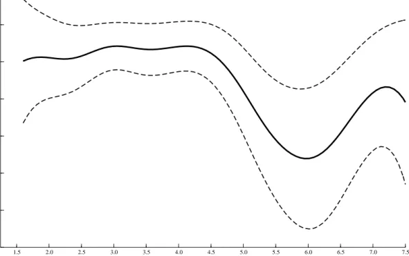
Figure 1 gives a graph of a nonparametric regression of the participation decision in the experiment on age. The participation probability remains close to 1 from the age of 16 to 40. From 40 onwards however, the participation probability significantly declines and reaches a low of 82% at the age of 60. Beyond 60 years of age, the participation probability increases again, although this rise is not statistically significant. As most non-participants did not mention any specific reasons for their decisions, we can offer some hypothetical explanations for the mid-life drop in participation. First, the natural explanation would be that non-participants have a higher opportunity costs of time. This interpretation is inconsistent with the descriptive evidence indicating that non-participants are both less involved in the labor market and do not have above average income. An alternative explanation would be that non-participants are more reluctant to get involved into cognitive demanding tasks. CentERdata keeps track of the time taken to answer any question they ask their members to answer. Table 1 displays some statistics on game completion time for all types of panel members contacted.
As expected, non-participants have the lowest participation time in the experiment at every point of the distribution, with a median time slightly greater than a minute. The distribution of time of play ofR dominates that of S players at every quartile, a 9Of the 42 non-participants, 14 of which had initially accepted to play but eventually backed out
of the experiment after having observed the roles they were assigned to play. It is interesting to note that 11 out of the 14 panel members who declined to participate after having observed their roles wereR players.
25th Median 75th IQR N Not Played 0.73 1.28 3.36 2.63 42
S 2.40 3.29 4.30 1.89 276 R 4.10 5.93 8.15 4.05 223
Table 1: Percentiles of the minutes spent playing the experiment. The Inter-Quartile-Range (IQR) is defined as the difference between the 75th percentile and the 25th percentile of the distribution.
result primarily due to the fact thatR players had to play the time-intensive strategy method. The interquartile range serves as a measure to judge inequality in a distri-bution. We find that R players not only took more time to play the experiment but that the distribution of their time of play is the most dispersed, followed by that of non-participants and that of S players. We mentioned previously that the unlimited answering time given to the participants allows for the possibility of group rather than individual decision making. Assuming that collective decision making takes time to complete, a high game time would be a source of concern. However, since the majority of players took less than 10 minutes to complete the experiment from the time they logged in the CentERdata network, it is unlikely that such collusive behavior is present.
2
The senders decision
2.1
Revealed versus stated trust behavior
We model trust as an unobserved continuous latent process. Let individual i’s unob-servable trust propensity T∗
i ∈ R be represented by the following linear single index form
Ti∗ =xti0βt+εti (1) wherext
i (K×1) is a vector of realizations of the observed characteristics of proposeri plus a constant term, βt (K×1) is the complete vector of unknown slope population parameters andβt∗ will be referred to as the vector of slope parameters excluding the
constant term. We observe two different discrete measures of trust for each individual, the yE
based on stated preferences based on answers to the WVS trust question. Both sets are defined as
YE = {0,1, ..., C}
YW V S = {0,1}
The categories correspond to the amount sent assuming that the individual trust propensity increases with higher amounts sent. We are interested in measuring the effects of background characteristics of trust. Both discrete measures can be thought of being generated from two distinct mappings from the real line to either YW V S or
YE. The ordered and binary response mapping functions (Maddala, 1983) yield the following choice probabilities
Pr¡yE i =j|xti ¢ = Pr¡ηj−1 < Ti∗ < ηj|xti ¢ for j = 0,1, ..., C (2) where{ηj−1}Cj=0are threshold parameters We make the following normalizationsη−1 =
−∞and ηC =∞. The probabilities of stating that one trusts is given by Pr¡yiW V S = 1|xti¢= Pr¡Ti∗ > η0|xti
¢
(3) In both models, η0 is not separately identified from the constant, we normalize it to
0. Under the assumption that εi is normally distributed with variance σ2 we obtain the familiar ordered and binary probit models. Allesina and La Ferrara (2002) use the binary probit to analyze individual responses to the WVS trust question. Implicit in their empirical model is the underlying latent trust propensity defined above. In par-allel, the ordered probit model has been used to analyze experimental trust responses in the BDM game. Here again the latent trust propensity is implicit in the empirical model.
In our design, senders answered the WVS trust question after having chosen yE i . This contrasts with Glaeser et al. who asked the WVS two months before the exper-iment took place. As we discussed in the previous section, there are advantages and disadvantages to both approaches. The main disadvantage of our approach is that senders have the possibility to reinforce their experimental decisions with their answer to the WVS question rather than to state their true underlying trust propensity. This
would induce a spurious resemblance between both measures. Two cases are worth mentioning. First, an individual who sent a large amount in the experiment may be more inclined to state that he trust others when in fact he would have answered nega-tive if the experiment had not taken place before hand. We denote the probability of this event as α10
¡
yE i
¢
. Secondly, some of the low senders may be more likely to state that they do not trust others when in fact they would have answered the opposite had the experiment not preceded the WVS question. Correspondingly, we denote the probability of this event as α01
¡
yE i
¢
. If either event occurs with positive probability, our WVS trust answers are potentially misclassified, where the magnitude and the di-rection of the misclassification would depend in part onyE
i . To investigate this claim, we generalize the binary probit model (3) to allow for the possibility of misclassifica-tion. Using the law of total probability, we can rewrite the probability of answering positively to the WVS trust question as
Pr¡yW V S i = 1|xti, yiE ¢ = Pr¡yW V S i = 1|Ti∗ ≥0, yEi ¢ ·Pr¡T∗ i >0|xti ¢ (4) + Pr¡yW V S i = 1|Ti∗ <0, yiE ¢ ·Pr¡T∗ i <0|xti ¢ = £1−α01 ¡ yE i ¢¤ ·Pr¡T∗ i >0|xti ¢ +α10 ¡ yE i ¢ ·Pr¡T∗ i <0|xti ¢ (5) Equation (5) shows that in the presence of misreporting, the probability that a sender states that he trusts others will be a weighted sum of the probability that he would really answer positively and that he would really answer negatively to the WVS ques-tion. In the absence of misclassification Pr¡yW V S
i = 1|xti, yiE
¢
= Pr (T∗
i >0|xti), which corresponds to truthful statement of preferences. It is important to note that the ex-perimental decision yE
i only affects answers to the WVS trust question via their effect on the misreporting probabilities. Put another way, the experiment does not directly affect the trust propensity of an individual but it affects his probability of misreport-ing his true intentions. We make the followmisreport-ing functional form assumptions on the misclassification probabilities α10 ¡ yiE¢ = exp ¡ θ10 0 +θ101 yiE ¢ exp (θ10 0 +θ101 yiE) + 1 α01 ¡ yE i ¢ = exp ¡ θ01 0 +θ011 yiE ¢ exp (θ01 0 +θ011 yiE) + 1
If θ10
1 = θ011 = 0 misclassification is random in the population of senders10 and is
not affected by the preceding experiment. This hypothesis can be tested using usual Wald type tests (e.g. Ruud, 2000). When (α10 =α01 = 0), senders truthfully answer
the WVS question. We test for this last hypothesis using the log-likelihood ratio test approach of Andrews (2001)11.
2.2
Comparing stated versus revealed preferences
A heavily debated topic is whether stated trust measures convey any information of the true underlying trust propensity of individuals. Glaeser et al. (2000) run a linear regression of yE
i onyW V Si and a set of covariates and find that the coefficient of yW V Si is not statistically significant. They interpret this result as evidence that stated trust measures are unreliable as the result of individual misreporting of their true trust intentions. This result has since been referred to as convincing evidence against the use of stated trust responses (Bowles and Gintes, 2002) . We now show that the Glaeser et al. test explores whether or not the unobserved component determining yW V S
i correlates with yiE. The proof of this result starts by writing down the following two linear probability models
yE
i = xti0βE +λyiW V S+εEi (6) yW V S
i = xti0βW V S+εW V Si (7) The first equation corresponds to the linear probability model estimated by Glaeser et al. where the experimental results are regressed on the observed characteristics and answers to the WVS trust question while the second equation relates answers to the WVS trust question to the same vector of observed characteristics. Substituting (7) in
10This is the model studied by Hausman et al. (1998).
11The parameter space of the misclassification probabilities is [0,1]×[0,1]. Under the null hypothesis
of no misclassification,α10=α01= 0 rests on the boundary of the parameter space. In this specific
case, it is known that the distribution of the LR test statistic is no longer a standard chi-square distribution. Andrews (2001) proposed a technique to simulate the true critical values of the LR test. For a recent application of this method, the reader is referred to Dustmann and van Soest (2003).
(6) yE i = xti0βE +λ ¡ xt0 i βW V S+εW V Si ¢ +εE i = xt0 i ¡ βE+λβW V S¢+λεW V S i +εEi = xt0 i βE++λεW V Si +εEi (8) whereβE+ =βE+λβW V S. Equation (8) clearly shows that testing λ= 0 amounts to testing whether εW V S
i correlates with experimental trust. Economically, it is unclear whether this correlation is of any interest. The literature comparing stated and revealed preference data has long recognized that the unobserved components of both types of data are likely to differ. Hence, the insignificant result found by Glaeser et al. can be difficultly interpreted. At a more fundamental level, it is more interesting to examine whether the inferences made on the joint effects of background characteristics on trust differ between both measures. This would require a test which compares the systematic part of the trust propensity across both models. The powerful feature of our empirical approach is to recognize that both experimental and WVS trust responses are modelled as being generated from the same underlying linear trust propensity (1). If all statistical assumptions of the model hold, Maximum Likelihood yields consistent estimates of βt/σ =©β1 σ, β2 σ, β3 σ, ..., βK σ ª
. As we just discussed, comparing βt/σ across both models is undesirable as σ2 in both models are related to unobservable components whose
difference have no clear behavioral interpretation. However, dividing βt/σ by say the second component β2 σ yields a vector βt/β2 = n β1 β2,1, β3 β2, ..., βK β2 o which is independent ofσ. This suggests fixing thek’th slope parameter to 1 or -1 and recovering consistent estimates of ξ =βt−/β
k (where βt− is the subset of βt which excludes the k’th slope parameter) both with the ordered and binary probit models.
Under the null hypothesis that the effects of background characteristics are the same, both sets of estimates would equal each other12. This forms the basis of a new
minimum distance test which simply evaluates whether there are sufficient statistical differences between both sets of estimates. Our test statistic has the following familiar 12The constant term parameter is generally not separately identified from the threshold parameters
in both the binary and ordered probit models. Given their values are function of the ad hoc threshold assumptions, they are not used in computation of the test.
quadratic form
N¡ξE−ξW V S¢0W−1¡ξE−ξW V S¢ ∼χ2(K −2)
where ξE and ξW V S denote the vector of parameters of the experimental and stated trust models andWrepresents the covariance matrix of the difference vectorξE−ξW V S. A proof of the consistency, asymptotic distribution and details on the computation of the test can be found in the appendix of the paper.
2.3
The reciprocity decision
Responders were asked to play the strategy method by which they state how much they will give back for each of the 11 possible amounts they can receive from the sender. This design implies that we observe for each responder an eleven dimensional vector yR yr = yr 0 ∈[0,500] yr 50∈[0,500 + 2×50] yr 100 ∈[0,500 + 2×100] ... yr 500 ∈[0,500 + 2×500] whereyr
0 denotes the amount the responder is willing to return when receiving 0
Cen-tERpoints from the sender, and so on. For any given individual, an increase inyr a asa increases may be due to the fact that the responder can return more and not because of the presence of genuine reciprocity. Since reciprocity is of primary interest, we remove this effect by dividing yr
a by the upper bound of the width of category a, expressing the amounts returned as percentages of the total possible amount sent for each cat-egory. Note, that this transformation only normalizes all responses to lay between 0 and 1. We model increase reciprocity as the increase in proportion of possible money returned asa increases. Let Ria ∈[0,1] for alla = 0,1,2, ...,10. Rescaling censors the data below at 0 and above at 1. We take this into account by first defining the ”true” underlying reciprocity propensity index
R∗
ia =xri0βr+λ(a) +εri (9) where xr
i (K ×1) is a vector of background characteristics of the receiver including the receiver’s age, income, level of education and his beliefs about the sender’s action.
The associated vector of unknown population parameters is βr (K ×1). Since all observed characteristicsxr
i are invariant across alla, any fixed effect type of estimation procedure would prevent us from estimatingβr, our focus parameters. We must then assume that any individual specific effect constant across all alternatives is captured by the covariatesxr
i. The parameter λ(a) is an a-sender specific constant term, allowing for shifts in levels between categories. Monotone reciprocity would imply the chain of estimates bλ(0) ≤ bλ(1) ≤ ... ≤ bλ(10). One could estimate the shift parameters by adding 10 fixed effects to the model. In the empirical application, we opt for a more parsimonious specification of the threshold model whereby λ(a) = γ1a+γ2a2
which reduces the amount of parameters to estimate from 10 to 2 (γ1, γ2).13 Given the
continuous nature of the density of the unobservable latent variable and the observed mixture of discrete and continuous observations, the observation rule is given by
Ria = max{0,xri0βr+λ(a) +εri} (10) In this paper, we consider two ways to recover estimates of βr and [γ
1, γ2]. If εri is homoscedastic and normally distributed, consistent estimates of Ξ = {βr, γ
1, γ2, σ2}
can be obtained by maximizing the Tobit (1958) likelihood function. Discussion of the properties of this estimator can be found in Maddala (1983). However, the Tobit model is generally quite sensitive to the specification of the error distribution (Goldberger, 1983, Arabmazar and Schmidt, 1982), likelihood-based estimators are in general in-consistent when the assumed parametric form of the likelihood function is incorrect. Furthermore, heteroscedasticity of the error term can also cause inconsistency of the parameter estimates even when the shape of the error density is correctly specified, as Hurd (1979) as shown. Our second estimator of (10) is the Symmetrically Trimmed Least Squares estimator (STLS) of Powell (1986). Contrary to Tobit, the STLS es-timator does not require normality and is robust to (bounded) heteroscedasticity of unknown form in εr
i, hence it is semiparametric. Moreover, it does not require that moments ofεr
i but simply thatεri is symmetrically distributed. Under the null hypoth-esis of normality and homoscedasticity of the error term, both the Tobit and STLS estimators consistently estimate the conditional mean of the latent process R∗
ia al-13We have estimated both the extended and parsimonious parametrization of the shift parameters
and found that both sets of results revealed the same monotonic paths. Results of the extended parametrization are available from the authors upon request.
though STLS will be relatively inefficient. Under the alternative that the error term is non-normal (but symmetric) and heteroscedastic, Tobit is inconsistent while STLS remains a consistent estimator of the model parameters. This will allow us to test the Tobit specification against non-normality and heteroscedasticity using a Hausman (1978) specification type test.
3
Empirical results
3.1
Trust
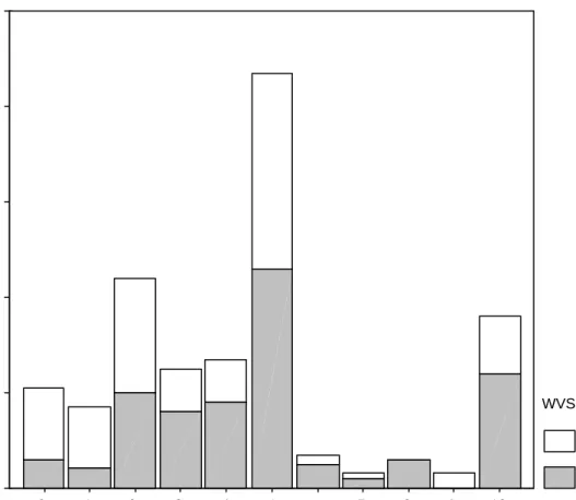
Figure 4 shows the distribution of revealed experimental responses for senders. The two distinctive features of this distribution are 1) the majority of subjects send positive amounts, contradicting self-interested behavior, 2) the distribution is heavily skewed to the left, with a mode at 5, the equal split category. The distributions of laboratory trust responses usually share both these characteristics, which implies at first glance that unconditional trust responses of our random sample of the Dutch population do not differ much from the unconditional distribution from samples drawn from student populations.
53% of our senders answered that most people can be trusted to the WVS trust question. To investigate whether senders who gave progressively more also tended to answer more positively to the WVS trust question, we plotted in each figure 4 the share of positive responses to the WVS trust question for each of the 11 categories sent. For individuals who have sent 0 or 1 unit, more than three quarters of them have reported negatively to the WVS trust question. This share progressively decreases from 2 units sent to 4 units sent. In category 5, i.e., sending half of the own endowment, senders are divided in their answers to the WVS trust question. This may be explained by being indifferent between giving a little or nothing and a lot or everything. In this case this category represents neutral actions as giving more is interpreted as signaling generosity while giving less is interpreted as making an unfair offer. This form of indecision could also explain the reported mix in answers. Finally, we find that 67% of those individuals who sent amounts above this indifference point have answered positively to the WVS trust question. These results combines indicate that there
seems to exist an unconditional relationship between stated and experimental trust. We now turn to the regression results which are presented in table 3. Due to little observations we join categories 6 to 9 and estimate an ordered probit model with eight categories (0=0 CP sent, 1=50 CP sent, 2=100 CP sent, 3=150 CP sent, 4=200 CP sent, 5=250 CP sent, 6=300, 350, 400, 450 CP sent, 7=500 CP sent). The table presents results from the ordered and binary probit models, each with three specifications. We include a vector of standard background characteristics such as age, income, education and religion in all six specifications.
The first 3 columns of the table are the ordered probit estimates of the experimen-tal responseyE
i . The first specification includes senders’ expected amount returned by their responders (STHINK) and senders’ estimate of the average amount that others will send (SMEANS) and the senders answer to the WVS trust question. The sec-ond specification omits the answer to the WVS trust question while specification 3 omits WVS and senders’ beliefs. The last two columns are the probit regressions of the WVS answers. Specification 4 contains the standard background characteristics and specification 5 is the probit model with misclassification due to the experimental response.
In analyzing our results, we will frequently compare them with results found in Allesina and La Ferrara (2002), Glaeser et al. (2002), Putnam (2000) and La Porta et al. (1997). It is important to note that both studies rely on organization membership of subjects as a proxy for social capital. In fact, Glaeser et al. motivate their approach precisely by referring to the Glaeser et al. (2000) finding that WVS trust answers were flawed as they do not correlate with experimental trust. Both experimental trust and organizational membership are likely to capture different concepts. Nevertheless, as trust and organizational membership are both believed to be important components of social capital, a comparison of our results to these studies will shed light on the robustness of the findings to the choice of proxy for social capital.
Before comparing results using experimental and survey trust measures, we test whether having senders answer the WVS trust question after having played would of affected their trust behavior. Specification 5 presents regression results where senders
are allowed to misreport their true answer to the WVS trust question and the size and magnitude of the misclassification. Both θ10
1 and θ011 associated with senders
experi-mental decisionyE
i are not significantly different from zero which indicate that senders experimental decision did not lead them to systematically misreport their true answer to the WVS trust question. There could still be random misclassification. The log-likelihood ratio test of Andrews (2001) based on specifications 4 and 5 has a value of 5.38 with 10% simulated critical value of 7.02, again not rejecting the null hypothesis of no-misclassification. These results seem to show that senders’ survey trust answers were not systematically affected by the experiment which preceded. Moreover, they also seem to show the absence of any form of misclassification, be it random or related to the preceding experiment.
Gender, individuals retired from the labor force or not working and all do not correlate with either experimental or WVS trust responses. This contrasts with the earlier findings of Glaeser et al. (2002) who find that women are less involved in organizations while income has a positive effect on organizational membership.
The age effect captured is robust and of similar magnitude across both the or-dered and binary probit specifications. Both age parameters are significant and of the expected sign reconfirming the concave life-cycle pattern usually found in the social capital literature (Putnam 2000, Glaeser et al. 2002).
The education profile differs remarkably between the experimental and the stated trust responses. Individuals with secondary and technical training are more likely to exhibit laboratory trust than subjects with either low education levels (the omitted category) and subjects with high levels of education. These findings tend towards an inverted U shape similar to that of age. Comparisons of specification 1 with speci-fication 2 and 3 show that this relationship is robust. On the other hand, however, this education profile is not at all present in the survey trust probit estimates. It is important to note that Glaeser et al. (2002) also find that organizational membership increases with education but does not find presence of non-linearities.
The impact of religion on trust remains a controversial issue in economics. La Porta et al. (1997) find that country specific religion indicators negatively affect trust
in a panel of countries. They rationalize this finding in terms of social norms and hierarchies that these religions impose. On the other hand, Allesina and La Ferrara (2002) find that the religion does not explain micro level answers to the WVS trust question. One reason for this apparent conflict is aggregation. Our regression results show that the effect of religion on trust is very much driven by the measure used. In the case of experimental data, we find no evidence of any systematic religious differences; this result holds across the different specifications. However, religious effects come out very significant in the WVS probit regressions. We find that catholics and protestants are less likely to report trusting others than individuals reporting to have other not having any religious beliefs.14 This finding is in line with those reported by La Porta
et al. (1997).
Participants in the role of senders were asked to state their beliefs about the response they expect to receive (STHINK) and their evaluations of what they think the average sender will send (SMEANS). Both variables have positive effects on trust and are highly significant. Apart from being statistically significant, these two variables alone improve the predictive fit of the model substantially, with a log-likelihood ratio statistic of 232.12 and a 5% critical value of 5.99 for a test of the null of no joint significance. These results would imply that senders who expected to receive more also sent more and those who thought other persons in the same role were going to send more to the responder increased the own amount sent. The latter result can be interpreted as a social norm while the former result captures expectations of the subjects.
The effect of senders lifetime experience with trust (TRUSTEXP) (see section 1 above) was recorded on a seven point scale. Somewhat like religion, reported experience with trust does not predict well subjects experimental trust responses but correlated remarkably well with the WVS trust answers, with a positive and significant effect.
Finally, we discuss the robustness of the Glaeser et al. (2000) finding that answers to the WVS trust questions do not correlate with experimental trust. The first two columns of table 3 show the regression results where the dummy variable WVS is added as a regressor. We find this variable to be significant at the 5% level using both Wald
and LR test procedures. On one hand, this result is not that surprising as we have seen in figure 4 that there was some form of parallelism between both measures, as those who have sent less in the experiment were relatively more likely to have answered negatively to the WVS. The notable differences between the Glaeser et al. study and the present one are that we asked the WVS-question after the experiment whereas Glaeser et al. weeks before. As we showed above, senders experimental decisions do not seem to have affected their truthful revelation of their survey trust answers. More importantly, we showed in section 2.2 that this correlation is difficult to interpret, as it implies that the unobservable factors explaining survey trust correlate with experimental trust, a correlation on which not much can be said.
The preceeding analysis has compared parameter estimates based on two different trust measures. We have found that the effect of religion and education may provide different information depending on the trust measure used. However, the similar age profiles and the similar insignificance of some other covariates imply that both trust measures may, for some covariates, provide the same information. In section 2.2, we introduced a new minimum distance test which tests for joint discrepancies between both measures. For our data, the test has a value of 6.78, with a 5% chi-square critical value of 22.36, clearly not rejecting the null hypothesis that the systematic part of the latent trust propensity is the same using both measures. This test result implies that the discrepancies between education and religion effects are not sufficient to overturn the similar age profiles and insignificant effects. This insignificance result could cause the possible low power of the test to detect some alternatives in a small sample. This issue is still a matter of investigation.
Before turning to the analysis of the responders choices, we briefly summarize the main points of this section. We made an effort to compare our findings to the existing social capital literature. This was primarily done to investigate robustness of the results to the proxy measure of social capital used. Our results show that experimental trust and organizational membership are likely to measure different behavioral characteristics of subjects. Nevertheless, as trust and organizational membership are both believed to be important components of social capital, our results suggest that estimation of gender, income and life cycle profiles will strongly be affected by which measure of
social capital used. This section also showed that contrary to Glaeser et al. (2000), the WVS trust answers seemed to be correlated rather well with our experimental measure of trust. Finally, we found that the presence of religion and education effects depend on whether or not we use experimental (revealed) or WVS (stated) trust measures but that those differences do not holt a jointly. Furthermore, subjects’ beliefs are important determinants of their trust actions while lifetime trust experience is not.
3.2
Reciprocity
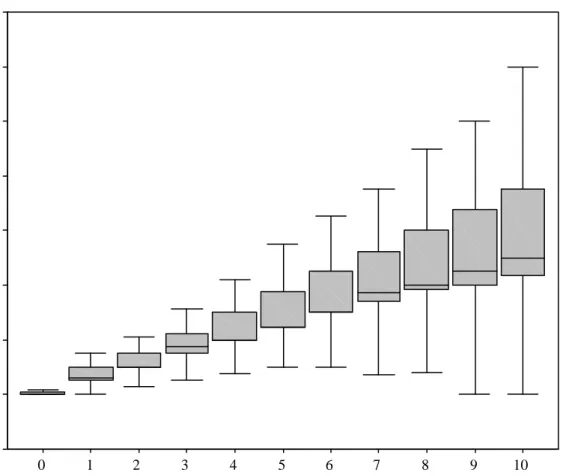
Figure 5 shows a boxplot of the average amounts returned for every possible unit the sender can choose to send. The two important elements of this figure are that amounts returned increase with the amounts sent and that the variability in the amounts re-turned increases with the amount sent. Figure 6 shows a boxplot of the normalized returns, i.e., the percentage returned out of the total possible amount ofRsent back to S. The general pattern remains the same, as this percentage monotonically increases with the amounts received.
We now turn to the econometric results of the responders model. Table 4 shows the regression results of the Tobit and the STLS estimators for two specifications of the reciprocity propensity. In the first specification, reciprocity is modelled as a func-tion of several background characteristics of the responder and their beliefs (RTHINK) about senders’ possible actions. The second specification allows for the possibility that subjects’ beliefs RTHINK, stated trust WVS and reported trust experience TRUST-EXP may vary with the age of the responders by including interaction terms. Both specifications were estimated using the parametric Tobit model and the semiparamet-ric STLS model. In both cases, the Hausman test statistic does not reject the null hypothesis of normality and homoscedasticity of the error terms15 on which the
To-bit model rests. To compare the specification with and without interaction terms, we computed a standard log-likelihood ratio test. The test value of 19.9 and a 1% critical value of 11.34 clearly rejects the parsimonious specification in favor of the specification with interaction terms. Given the relative efficiency of Tobit over STLS under the null 15For the two specification presented in table 4, the Hausman test statistic is respectively 3.107 and
hypothesis and our specification tests, our analysis will focus on the results from the Tobit model.
The parameters of γ1 and γ2 correspond to the vector of units sent to the receiver
and its square. They are indicative of the path of the shift parametersλ(a). As could be seen from the raw data in figure 5, the estimates show thatλ(a) are increasing and progressively diminishing overa, a clear indication of monotonically concave reciprocity as responders give systematically more for each unit received. This is also reflected in the Tobit estimates. We find that the mean conditional reciprocity is increasing and concave in the amounts received.
The life cycle evolution of reciprocity is captured by the parameters of RETIRED, AGE, AGESQ and the three interaction terms. The change in the conditional mean return propensity which follows from a change in age is given by
∂R∗
ia ∂AGEi
=−0.0014
(0.0014) + 0.000032(0.000017) AGEi−0.0014(0.0005) WVSi−0.0003(0.0000) RTHINKi (11)
This indicates that participants tend to reciprocate less as they get older but at a decreasing rate. Additionally, those who report trusting others and who believe that they will receive more tend to return on average less as they get older. It is important to note, that this result only reports the average response. In a quantile regression analysis of the response behavior, Bellemare and Kr¨oger (2003b) (Bellemare and Kr¨oger 2003b) show that individuals returning the most increase their share returned as they get older.
These results differ remarkably from the life cycle patterns observed in the trust responses where trust was shown to be strictly decreasing and concave with age. The education pattern also seems to reflect an opposite picture than for trust. We find that educated subjects tended to return significantly less than non-educated subjects with no significant differences between secondary, training or university level education.
Contrary to the trust results documented earlier were gender did not appear to play an important role, we find that men return on average significantly less than women. There are nevertheless some areas where trust and reciprocity have concomitant effects. We do not find any relationship between income, work status, retirement status and
lifetime trust experience to correlate with reciprocity. Similarly to experimental trust results, religion effects seem to be absent. RTHINK measures the beliefs of responders what they expect their matched sender will eventually send to them. We find that those responders who believed they would receive more increased the proportion they are willing to return. Finally, we find that those who reported trusting more others were also more likely to return more to the senders. This fact supports the findings in Glaeser et al. (2000) were the same relationship was shown to exist.
The main conclusions of this section are the following. First, age and education profiles of reciprocity were shown to be at odds with those of the trust propensity. We find that higher educated subjects trust more but return less and that trust decreases with age while reciprocity does exactly the opposite. Second, we have found that men tend to reciprocate significantly less than women. Despite these differences, there are nonetheless similarities between both trust and reciprocity behavior. First, life time experience with trust, religion, income and work and retirement status do not correlate with reciprocity while subjects’ beliefs are shown to be significant determinants of reciprocity. Furthermore, stated trust answers to the WVS question correlate with trustworthiness. This confirms previous findings in this literature.
3.3
Participation
Once contacted by CentERdata concerning our experiment panel members could decide whether or not to participate. The reasons for participating in laboratory experiments, especially the impact of financial rewards, have been analyzed in several meta studies (Smith and Walker, 1993?, Hertwig and Ortmann, 2001, Camerer and Hogarth, 1999). But also the impact of voluntary participation (Eckel and Grossmann, 2000) has been of interest for investigation. There has always been a fear that experimental subject pools are non-random samples of the population of interest. Amongst the most cited explanations of this non-randomness are that participants might be motivated intrin-sically (Camerer and Hogarth), e.g., have above average taste for gambling and risk or higher cognitive abilities . The crucial question is whether or not non-randomness of participants based on these traits feeds itself into non-randomness in the experimental
outcomes.16
Usually investigation of participation bias is limited by two data-shortcomings. First, some of the traits affecting participation are mostly unobservable to the ex-perimenter, often because they are difficultly measurable. Secondly, experimenters generally do not have any information on non-participants, preventing any possible control for their effects without further combinations of additional information and as-sumptions (see Manski, 1999). Because of these data limitations, tests of participation bias in laboratory-type experiments are scarce.
CentERdata uses a common method and selects CP members after certain criteria to ensure the representativeness of the Dutch population of the CP. The approached households are asked to participate in the panel (see section 1). Camerer and Hogarth mention that beside monetary incentives also intrinsic motivations play an important role to guide the attraction to participate in laboratory experiments, which is certainly the case for other scientific investigations like survey investigations. The incentives for Dutch persons to participate in the CP are not monetary. They receive a reim-bursement for their telephone allowances while connected to CentERdata to answer the questionnaires. In this light, we probably face an already intrinsically highly motivated sample and thereby we might exhibit even a larger participation rates when asking to join and interact in an experiment with financial rewards than one would expect in the real field. Nevertheless, 7% of the panel members approached decided not to partici-pate. In our experiment, non-participants are observable CP members with observable background characteristics. This allows us to test whether or not participants behaved in a non-random manner.
We test for participation bias in the framework developed by Heckman (1978)17. Let
di ∈ {0,1}be an indicator of participation in the experiment and let the an individuals 16The statistical dependance between the experimental outcome and the participation decision
implies that Pr (Y|x, d= 1)6= Pr (Y|x) whereY is the random outcome of an experiment andxare some conditioning characteristics. This inequality says that the probability distribution of observed outcomes of participants will differ from that of randomly assigned participants to the experiment, given x. This result holds generally for the Ordered Probit model with the experimental measure
¡
Y =yE
i ,x=xti
¢
, the Binary Probit on the survey trust measure¡Y =yW V S
i ,x=xti
¢
and the Tobit model of the responders decision (Y =Ria,x=xri).
unobserved latent propensity to participate. d∗
i =xjiδ+θRATIOi +εdi for j =r,t
where xji is the conditioning vector entering the trust and reciprocity models, εd i is an unobservable N(0,1) component driving participation and (δ,θ) are unknown pop-ulation constants. A general feature of these models is the requirement of a valid exclusion restriction for nonparametric identification of the selection bias. In practical terms, we need a variable which affects participation but not directly the experimen-tal and survey responses. We computed the variable RATIO, which is the number of questionnaires completed to the total number of questionnaires submitted to a CP member in the three months which preceded our experiment. The dependance between the experimental outcomes and the participation decisions is captured by the amount of correlation between εd
i and the unobservable componentsεti in trust propensity (for t=E and W V S, see equation (1)) andεr
i in the reciprocity propensity (see equation (9)). For the trust responses, we estimated separately both the ordered probit and bi-nary probit models jointly with the selection equation. We estimated the Tobit model with selection for the reciprocity decisions.
The presence of participation bias can be determined by testing the statistical significance of all three correlation coefficients. In all three cases we did not find any correlation coefficients to be significantly different from zero, which implies the absence of selection bias in our data. Most of parameters entering the systematic part of the participation propensity were insignificant. One notable exception was income which came out with a positive and significant effect on participation. Absent the income effect, we conclude that participation in our experiment seems to be mostly driven by unobserved heterogeneity which does not correlate with the experimental decisions.
4
Conclusions
Up till now, the microeconometric analysis of trust has relied on one of two complemen-tary methodologies. Survey methods on one hand collect responses of heterogeneous samples, at the expense of having to rely of hypothetical and self-reported measures.