Local influence diagnostics for generalized linear mixed models with overdispersion

(1)

For Peer Review Only

Local Influence Diagnostics for Generalized Linear Mixed Models With Overdispersion

Journal: Journal of Applied Statistics Manuscript ID CJAS-2015-0173.R1

Manuscript Type: Original Article Date Submitted by the Author: 24-Feb-2016

Complete List of Authors: Rakhmawati, Trias Wahyuni; I-BioStat, Universiteit Hasselt,

Molenberghs, Geert; I-BioStat, Universiteit Hasselt, ; I-BioStat, Katholieke Universiteit Leuven,

Verbeke, Geert; I-BioStat, Katholieke Universiteit Leuven, ; I-BioStat, Universiteit Hasselt,

Faes, Christel; I-BioStat, Universiteit Hasselt, Keywords:

Case deletion, Combined model, Logit-normal model, Poisson-normal model, Probit-normal model, Weibull-normal model

<a href="http://www.ams.org/mathscinet/msc/msc2010.html" target="_blank">2010 Mathematics Subject Classification</a>:

62F99, 62P10

(2)

For Peer Review Only

To appear in theJournal of Applied Statistics

Vol. 00, No. 00, Month 20XX, 1–20

Local Influence Diagnostics for Generalized Linear Mixed

Models With Overdispersion

Trias Wahyuni Rakhmawatia∗ Geert Molenberghsa,b _{Geert Vebeke}b,a _{Christel Faes}a,b

a_{I-BioStat, Universiteit Hasselt, B-3500 Hasselt, Belgium} b_{I-BioStat, KU Leuven, B-3000 Leuven, Belgium}

(Received 00 Month 20XX; accepted 00 Month 20XX)

Since the seminal paper by Cook and Weisberg [9] , local influence, next to case deletion, has gained popularity as a tool to detect influential subjects and measurements for a variety of statistical models. For the linear mixed model the approach leads to easily interpretable and computationally convenient expressions, not only highlighting influential subjects, but also which aspect of their profile leads to undue influence on the model’s fit [17]. Ouwens, Tan, and Berger [24] applied the method to the Poisson-normal generalized linear mixed model (GLMM). Given the model’s non-linear structure, these authors did not derive interpretable components but rather focused on a graphical depiction of influence. In this paper, we consider GLMMs for binary, count, and time-to-event data, with the additional feature of accommodating overdispersion whenever necessary. For each situation, three approaches are considered, based on: (1) purely numerical derivations; (2) using a closed-form expression of the marginal likelihood function; and (3) using an integral representation of this likelihood. Unlike when case deletion is used, this leads to inter-pretable components, allowing not only to identify influential subjects, but also to study the cause thereof. The methodology is illustrated in case studies that range over the three data types mentioned.

Keywords:Case deletion; Combined model; Logit-normal model; Poisson-normal model; Probit-normal model; Weibull-normal model.

1. Introduction

Next to linear mixed models (LMM) for hierarchical Gaussian data [26], generalized linear mixed models (GLMM; [2, 19, 28]) have become a standard tool for the analysis of hierarchical data of a variety of data types. Routinely, after formulating and fitting a model, an assessment of model fit and a diagnostic analysis is advisable. Here, we are concerned with the detection of influential subjects.

A large variety of diagnostic tools is available for (generalized) linear models. Cook and Weisberg [9] and Chatterjee and Hadi [3] provide early treatises. In linear regres-sion, Cook’s distances [5–7] have been used extensively. They capture how much a pa-rameter changes based on the contribution from one particular individual. If unduly large, the subject is considered influential. Linear mixed models, unlike linear models, generally do not allow for closed-form parameter estimators. Further, residual analysis is not straightforward, given the presence of both fixed- and random-effects, so that even uniquely defining residuals is not possible. For these and related reasons, Lesaf-fre and Verbeke [17] , chose local influence [1, 8] to examine influence in linear mixed models. Lesaffre and Verbeke [17] studied how much case-weight perturbation impacts

∗_{Corresponding author. Email: [email protected]}

1 2 3 4 5 6 7 8 9 10 11 12 13 14 15 16 17 18 19 20 21 22 23 24 25 26 27 28 29 30 31 32 33 34 35 36 37 38 39 40 41 42 43 44 45 46 47 48 49 50 51 52 53 54 55 56 57 58

(3)

For Peer Review Only

parameter estimates; such perturbations refer to infinitesimal deviations from a subject’s contribution to the log-likelihood. Their proposal has several attractive features. First, it distinguishes influence in fixed-effects parameters from that in variance components. Second, for each of these parameter subsets, influence is decomposed in interpretable components. Third, the influence diagnostics are computationally inexpensive, once the mixed model is fitted.

The GLMM has received less attention, even though Ouwens, Tan, and Berger [24] ap-plied local influence to count data. An important complication is that the (log-)likelihood function does not admit a closed form. Hence, their derivations were numerical in nature, which makes it less evident to derive meaningful influence components.

Here, we extend local influence for the GLMM in several ways. First, we consider out-comes of binary, count, and time-to event type. Second, using the extension proposed by

Molenberghs, Verbeke, and Dem´etrio [20] and Molenberghs et al [21], we flexibly allow

for overdispersion in the GLMM, by introducing conjugate random effects, in addition to normal ones. This model is referred to as the combined model. Third, apart from numerical derivations of local influence, we examine two alternative routes: (a) closed

forms for the marginal likelihood such as proposed in Molenberghset al [21] and (b) the

marginal likelihood with integral form. The closed forms in (a) do not always exist; while they are available for the probit-(beta-)normal, Poisson-(gamma-)normal, and Weibull-(gamma-)normal, they are not for the logit-(beta-)normal. Even when they do, they may be somewhat unwieldy and therefore, route (b) is more promising. Fourth, interpretable components are derived, allowing to get a better perspective on the data-analytic conse-quences of candidate influential subjects. In other words, once influential subjects have been identified, it can be examined precisely which aspects lead to such influences.

The paper is organized as follows. In Section 2 four case studies are introduced, two counts, one made up of binary, and one of time-to-event type. Their analyses are reported in Section 6. Section 3 describes the generalized model based on the exponential family. Section 4 reviews the essence of local-influence theory. The LMM case is sketched in Section 5.1, and we show that using the integral form of the log-likelihood leads to exactly the same expressions. The Poisson, probit, logit, and Weibull cases are studied in Sections 5.2–5.5.

2. Case Studies

2.1 A Clinical Trial in Epileptic Patients

The data considered here are obtained from a randomized, double-blind, parallel group multi-center study for the comparison of placebo with a new anti-epileptic drug (AED),

in combination with one or two other AED’s. The study is described in Faught et al

[12]. The randomization of epilepsy patients took place after a 12-week baseline period that served to stabilize the use of AED’s, and during which the number of seizures were counted. After that period, 45 patients were assigned to the placebo group, 44 to the active (new) treatment group. Patients were then measured weekly. Patients were followed during 16 weeks, after which they were entered into a long-term open-extension study. Some patients were followed for up to 27 weeks. The outcome of interest is the number of epileptic seizures experienced during the most recent week. The research question is whether or not the additional new treatment reduces the number of epileptic seizures. 1 2 3 4 5 6 7 8 9 10 11 12 13 14 15 16 17 18 19 20 21 22 23 24 25 26 27 28 29 30 31 32 33 34 35 36 37 38 39 40 41 42 43 44 45 46 47 48 49 50 51 52 53 54 55 56 57 58

(4)

For Peer Review Only

2.2 Headache Study

This dataset has been reported by McKnight and Van Den Eeden [18]. The experi-ment has been done using a two-treatexperi-ment, double-blind crossover design; the number of headaches per week is repeatedly measured during 5 weeks of experiment. The study objective was to investigate whether aspartame causes headaches in subjects who believe they experience aspartame-induced headaches. Twenty-seven volunteers who responded to newspaper advertisements were randomized to one of four treatment regimens. Each regimen began with a seven-day placebo run-in period followed by four treatment peri-ods of seven days each. Each treatment period was separated by a “washout day.” Both aspartame (A), given at 30 mg/kg/day, and placebo (P) were administered in capsules of three doses per day. The four possible orderings of treatment after the run-in period were APAP, APPA, PAPA and PAAP. Most of the run-in periods were done within 7 days, yet some of the periods were smaller.

2.3 A Clinical Trial in Onychomycosis

These data come from a randomized, double-blind, parallel group, multicenter study for the comparison of two oral treatments (A and B) for toenail dermatophyte onychomy-cosis (TDO; [10]). TDO is a common toenail infection, difficult to treat, with prevalence exceeding 2% [25]. Anti-fungal compounds, classically used for treatment of TDO, need to be taken until the whole nail has grown out healthily. The development of such new compounds, has reduced the treatment duration to 3 months. The aim of the present study was to compare the efficacy and safety of 12 weeks of continuous therapy with A or B. Twice 189 patients were randomized. Subjects were followed during 3 months of treatment and followed further until month 12. Measurements were taken at 0, 1, 2, 3, 6, 9, and 12 months. The outcome of interest is severity of infection (0: severe; 1: non-severe). The estimand is the difference in slope over time between the arms.

2.4 Recurrent Muscle Soreness

These data come from Hosmer and Lemeshow [14]. The study of two treatment modal-ities was aimed at reducing the occurrence of muscle soreness among 400 middle-aged men in the beginning of weight training. Subjects were randomized over two instruc-tional programs designed to prevent muscles soreness. The control treatment consisted of standard written brochures and instructions used by the health club to explain the proper technique, including the suggestions for frequency and duration of training. The new method included 1 hour with a personal trainer as well as brochures. The subjects were followed for some time and the dates on which muscles soreness limited the pre-scribed workout were recorded, converted to number of days between soreness episodes. All subjects had between one and four muscle soreness episodes. The start and end of each episode is recorded, together with the status indicator to denote whether the end of the episode corresponds to a muscle soreness or not.

3. Generalized Linear Mixed Models

The generalized linear mixed model [2, 11, 28] is arguably the most frequently used random-effects model in the context of (non-)Gaussian repeated measurements, extend-ing both generalized linear models for univariate outcomes and linear mixed models [26]. Let Yij be the jth outcome for subject i= 1, . . . , N, j = 1, . . . , ni and group the ni

1 2 3 4 5 6 7 8 9 10 11 12 13 14 15 16 17 18 19 20 21 22 23 24 25 26 27 28 29 30 31 32 33 34 35 36 37 38 39 40 41 42 43 44 45 46 47 48 49 50 51 52 53 54 55 56 57 58

(5)

For Peer Review Only

measurements into vector Yi. Assume that, given q-dimensional random effects

bi ∼N(0, D), (1)

the Yij’s are independent with model

fi(yij|bi,ξ, φ) = exp φ−1[yijλij −ψ(λij)] +c(yij, φ) , η[ψ0(λij)] =η(µij) =η[E(Yij|bi,ξ)] =x0ijξ+z 0 ijbi (2)

for a known link function η(·), with xij and zij p- and q-dimensional vectors of known

covariate values, ξ a p-dimensional vector of unknown fixed regression coefficients, and

withφa scale (overdispersion) parameter. Letφ(bi|D) be the multivariate normal density

with mean 0 and varianceD. The marginal likelihood function is:

L(ϑ, D) = N Y i=1 Z ni Y j=1 fij(yij|ϑ,bi) φ(bi|D) dbi.

Here,ϑ groups all parameters in the conditional model forYi given the random effects.

Not always is there a closed form for the integral in (3), nor for the corresponding moments. The most notorious counterexample is the logit-normal model, where (2) uses the logit link. While a suite of computational techniques has been derived to approximate the likelihood numerically, e.g., using Taylor series expansions and numerical integration, it poses further challenges when additional calculations are requested. We are in this position, because local influence starts from the likelihood (see Section 4).

3.1 The Linear Mixed Model for Gaussian Data

The hierarchically specified linear mixed-effects model takes the form [26]:

Yi|bi∼N(Xiξ+Zibi,Σi), (3)

where ξ is a vector of fixed effects, and Xi and Zi are design matrices. The rows of

Xiξ +Zibi are made up by the linear predictors (2). Evidently, bi is as specified in

(1). The corresponding marginal model, needed for maximum likelihood estimation and hence the corner stone for local influence [17] obtains easily and is, again, of a multivariate normal form:

Yi ∼N(Xiξ, Vi =ZiDZi0+ Σi). (4)

3.2 The Poisson-Normal and Poisson-Gamma-Normal Models for Count Data

From the general developments above, the Poisson-normal model is:

Yij ∼Poi(λij), (5) λij = exp x0ijξ+z 0 ijbi , (6) 1 2 3 4 5 6 7 8 9 10 11 12 13 14 15 16 17 18 19 20 21 22 23 24 25 26 27 28 29 30 31 32 33 34 35 36 37 38 39 40 41 42 43 44 45 46 47 48 49 50 51 52 53 54 55 56 57 58

(6)

For Peer Review Only

and bi as in (1). Molenberghs, Verbeke, and Dem´etrio [20] and Molenberghs et al [21]

derived a closed form for the marginal model:

P(Yi =yi) = 1 Qni j=1yij! X t (−1)Pnij=1tj Qni j=1tj! ·exp   ni X j=1 (yij+tj)x0ijξ   ×exp    1 2   ni X j=1 (yij +tj)z0ij  D   ni X j=1 (yij+tj)zij      . (7)

The vector-valued index t= (t1, . . . , tni) ranges over all non-negative integer vectors.

When overdispersion is accommodated, as in Molenberghs, Verbeke, and Dem´etrio [20]

and Molenberghs et al [21]), (5) changes to

Yij ∼Poi(θijλij), (8)

with λij as in (6) andθij ∼Gamma(αj, βj). The joint distribution now is:

P(Yi =yi) = X t   ni Y j=1 yij+tj yij · αj+yij+tj −1 αj−1 ·(−1)tj_·_βyij+tj j   ×exp   ni X j=1 (yij +tj)x0ijξ   ×exp    1 2   ni X j=1 (yij+tj)z0ij  D   ni X j=1 (yij +tj)zij      . (9)

For identification, write βj = 1/αj. The modeler may chooseαj and βj terms free of j.

While Zeger, Liang, and Albert [29] derived a closed form for the mean function only,

Molenberghs et al [21] thus provided closed forms for all of the moments and for the

joint marginal distribution; they did so for the combined-model extension of the GLMM, and hence for the GLMM itself. This opens avenues for local influence and corresponding interpretable components, which goes well beyond what was done in the literature thus far (e.g., [24]).

3.3 The Probit-Normal Model for Binary and Binomial Data

A probit-normal model is specified by Yij ∼Bin(λij, nij) and

λij = Φ1(x0ijξ+z0ijbi). (10)

Molenberghs et al [21] showed that the marginal joint distribution is:

fni(yi =1) = Φni(Xiξ;L −1 ni), (11) with Lni =Ini−Zi D −1₊_Z0 iZi −1

Z_i0. Of course, this is only the probability of a

(so-called success) sequence consisting of ones. All other joint probabilities are derived by

1 2 3 4 5 6 7 8 9 10 11 12 13 14 15 16 17 18 19 20 21 22 23 24 25 26 27 28 29 30 31 32 33 34 35 36 37 38 39 40 41 42 43 44 45 46 47 48 49 50 51 52 53 54 55 56 57 58

(7)

For Peer Review Only

the usual combination rules [21]. When overdispersion is allowed for, then again λij is

multiplied by θij ∼Beta(α, β) and the joint distribution becomes:

fni(yi =1) = α α+β ni ·Φni(Xiξ;L −1 ni) (12)

Should the logit link be used, there is no closed form available. Of course, the approxi-mation rule for the logit by the probit function can be used [16, 21, 29]:

fni(yi=1)≈Φni cXiξ;Le−_n1 i , (13) with Le_n_i =I_n_i−c2Z_i D−1+Z_i0Z_i −1 Z_i0 and c= (16√3)/(15π).

3.4 The Weibull-Normal Model for Time-to-event Data

In the Weibull case, the corresponding model is

f(y_i|θi,bi) = ni Y j=1 λρy_ijρ−1ex0ijξ+z0ijbi_e−λyρijex 0 ijξ+z0ijbi , (14)

with bi as in (1). The joint distribution is [21]:

f(y_i) = X (t1,...,tni) ni Y j=1 (−1)tj tj! λtj+1_ρy(tj+1)ρ−1 ij ×exp (tj+ 1) x0_ijξ+1 2(tj+ 1)·z 0 ijDzij . (15)

Similar to the Poisson case, (t1, . . . , tni) ranges over all non-negative integer vectors.

When overdispersion is allowed for, the Weibull-Gamma-Normal model is:

f(y_i|θi,bi) = ni Y j=1 λρθijyρij−1ex 0 ijξ+z 0 ijbi_e−λyijρθijex 0 ijξ+z0ijbi , (16)

with now also θij ∼Gamma(αj, βj), leading to the closed form:

f(y_i) = X (t1,...,tni) ni Y j=1 (−1)tj tj! Γ(αj+tj+ 1)β_jtj+1 Γ(αj) λtj+1_ρy(tj+1)ρ−1 ij ×exp (tj+ 1) x0_ijξ+1 2(tj+ 1)·z 0 ijDzij . (17) 1 2 3 4 5 6 7 8 9 10 11 12 13 14 15 16 17 18 19 20 21 22 23 24 25 26 27 28 29 30 31 32 33 34 35 36 37 38 39 40 41 42 43 44 45 46 47 48 49 50 51 52 53 54 55 56 57 58

(8)

For Peer Review Only

4. Review of General Theory for Local Influence

4.1 Standard Approach

Local influence was presented by Cook [8] and used by many authors since. The impact of individuals and measurements on the analysis is assessed by comparing standard max-imum likelihood estimates with those resulting from slightly perturbing the contribution of an individual or measurement. The method is to be contrasted with global influence (case deletion), where impact is assessed by simply deleting an individual or measure-ment. While local influence comes with a certain amount of technicality, it is easy and fast to calculate, and in many cases leads to interpretable components of influence. The existence of such interpretable components is often, and also here, a major rationale for using the method. Lesaffre and Verbeke [17] introduced influence assessment for the lin-ear mixed model. A review of several diagnostic procedures for the linlin-ear mixed model is

given in Mun and Lindstrom [22]. Verbeke et al [27] used local influence for longitudinal

Gaussian data with dropout, while incomplete binary data were studied by Jansen et

al [15]. Verbeke and Molenberghs [26] and Molenberghs and Verbeke [19] reviewed the

method and provide ample references.

Ouwens, Tan, and Berger [24] applied local influence to the Poisson-normal model. We will follow their steps, but with extensions in three directions. First, we will provide closed-form expressions, based on an analytical form for the marginal likelihood function, as well as based on an integral form for the said likelihood. Second, we consider three important cases: binary, count, and time-to-event. Third, extensions will be constructed to allow for overdispersion in all of these settings. Some authors considered specific extensions as well. For example, Chen, Fu, and Wang [4] considered local influence for zero-inflated Poisson mixtures.

Let the log-likelihood for the generalized linear mixed model or its combined extension take the form

`(θ) =

N

X

i=1

`i(θ), (18)

in which `i(θ) is the contribution of the ith individual to the log-likelihood. Let

`(θ|ω) =

N

X

i=1

ωi`i(θ), (19)

now denote the perturbed version of `(θ), depending on an N-dimensional vector ω of

weights, assumed to belong to an open subset Ω of IRN. The original log-likelihood (18)

follows forω=ω0= (1,1, . . . ,1)0. Other perturbation schemes are possible [26]. Letθbbe

the maximum likelihood estimator forθ, obtained by maximizing`(θ), and letbθ_ω denote

the estimator for θunder`(θ|ω). Cook [8] proposed to measure the distance betweenθb_ω

and θb by the likelihood displacement: LD(ω) = 2

`(θˆ)−`(θˆω)

. LD(ω) will be large

if`(θ) is strongly curved atθb. A graph of LD(ω) versusωbrings out information on the

influence of case-weight perturbations. The graph is the geometric surface formed by the

values of the (N + 1)-dimensional vector

ξ(ω) = ω LD(ω) 1 2 3 4 5 6 7 8 9 10 11 12 13 14 15 16 17 18 19 20 21 22 23 24 25 26 27 28 29 30 31 32 33 34 35 36 37 38 39 40 41 42 43 44 45 46 47 48 49 50 51 52 53 54 55 56 57 58

(9)

For Peer Review Only

asωvaries throughout Ω. Following Cook [8] and Verbeke and Molenberghs [26], we will

refer to ξ(ω) as an influence graph.

Zhu and Lee [30] and Zhu et al. [31] proposed another approach to deal with the measurement of the distance between bθ_ω andθb. Instead of using the

observed-data log-likelihood, their method is applied to the objective func-tion that features in the expectafunc-tion step of the EM algorithm. Because this function is usually denoted by Q, their method is known as Q-displacement. In this paper, we focused on the used of the likelihood displacement LD(ω)

[8].

Cook [8] derived a convenient computational scheme. Let ∆i be the s-dimensional

vector of second-order derivatives of `(θ|ω), w.r.t. ωi and all components of θ, and

evaluated at θ =bθ and ω =ω₀. Also, write ∆ for the s×r matrix with ∆_i in the ith

column. Let ¨Ldenote the s×smatrix of second derivatives of `(θ), evaluated atθ =bθ.

For any unit vectorh in Ω, it follows that:

Ch = 2 h 0 ∆0L¨−1∆h . (20)

Various choices for h have received attention. First, as will be done here, one can focus

on subject ionly, by choosing h=hi, the zero vector with a sole 1 in theith position.

Local influence then is

Ci ≡ Chi = 2 ∆ 0 iL¨−1∆i . (21)

Second, h = hmax can be considered, the direction of maximal normal curvature [26].

Expressions can be derived when only a sub-vector of the parameter vector is of interest. See Supplementary Materials (Section S.1).

4.2 Proceeding When Faced With a Complicated Likelihood

As will be reviewed in Section 5.1.1, Lesaffre and Verbeke [17] proceeded by deriving local influence based on the explicit expression of the marginalized linear mixed model. While there are marginal expressions available for the Poisson, probit, and Weibull cases (Sections 3.2–3.4), these are involved. This is why we also proceed in two alternative ways. The first one consists of using integral expression (3), essentially combined with the property that integration and derivation can be interchanged under mild regularity conditions. Importantly, this route still allows for the derivation of interpretable compo-nents. A further alternative consists of choosing a fully numerical route, as in Ouwens, Tan, and Berger [24].

5. Local Influence for Generalized Linear Mixed and Combined Models 5.1 Local Influence for the Linear Mixed Model

5.1.1 Standard Approach, Based on the Marginal Likelihood

The backdrop for our developments is the method as derived for the linear mixed model [26]. They started from the marginal likelihood (4) directly. For this model, this is easy to do and hence a natural choice. We will review their derivations, with details relegated to the Supplementary Appendix Materials (Section S.2). We will then proceed alternatively

1 2 3 4 5 6 7 8 9 10 11 12 13 14 15 16 17 18 19 20 21 22 23 24 25 26 27 28 29 30 31 32 33 34 35 36 37 38 39 40 41 42 43 44 45 46 47 48 49 50 51 52 53 54 55 56 57 58

(10)

For Peer Review Only

by an integral-based approach. This will provide the basis for the analogous calculations in the non-Gaussian cases.

For the covariance structure, we assume conditional independence, i.e., Σi = σ2Ini,

with Ini theni×ni identity matrix.

It is advantageous that Ci admits closed form (21). Lesaffre and Verbeke [17]

de-composed Ci into five interpretable components. Let Ri,Xi, and Zi denote the

“stan-dardized” residuals and covariates for the ith individual, defined by Ri = V_i−1/2ri,

Xi =V_i−1/2Xi, andZi =V_i−1/2Zi, respectively, withri =yi−Xibξ. Further, for a matrix

A, letkAk=ptr(A0A) be the Frobenius norm of A [13]. The interpretable components

in Ci are then

kXiXi0k, kRik, kZiZi0k, kI −RiRi0k, kV_i−1k. (22)

First,kXiXi0kmeasures the “length” of the standardized covariates in the mean structure

and kR_ik is an overall measure for how well the observed data for the ith subject are

predicted by the mean structureXiξ. Second, the componentskZiZi0kandkI−RiRi0k

have a similar meaning, but then for the covariance structure. For example,kI−R_iR_i0k

will be zero only if Vi equals riri0. Note that riri0 is an estimate for var(yi), which

only assumes the mean to be correctly modeled as Xiξ. Therefore, kI −RiRi0k can

be interpreted as a residual, capturing how well the covariance structure of the data is

modeled by Vi =ZiDZi0+σ2Ini. Finally, the fifth component kV

−1

i k will be large if Vi

has small eigenvalues, indicating that the ith subject has little variability.

The decomposition of Ci immediately suggests a practical procedure to find an

ex-planation for the influential nature of an individual, i.e., when Ci is large, we examine

the diagnostics. Such plots are useful to graphically inspect the individuals in view of

their influence. Thus, it is sensible to start with an index plot of Ci. Following this, the

index plots of (22) can be examined. A recurrent practical difficulty with diagnostics is to establish a threshold above which an individual is defined as “remarkable.” It follows from (21) that N X i=1 Ci=−2 tr L¨−1 N X i=1 ∆i∆0i ! ,

which converges to 2s, for N approaching infinity. As with leverage in linear regression

[23, pp. 395–396], one could classify an individual for which Ci is larger than twice the

average value (larger than 4s/N, for N large) as influential. However, unlike for the

leverage situation, 2sis only the approximate sum of the Ci, which will not be accurate

if the model is not correctly specified (such that ¨L−1PN

i=1∆i∆

0

i does not converge to

Is) or if N is too small for the asymptotic results to be reliable. In such cases, Lesaffre

and Verbeke [17] proposed to replace 2sby the actual sum; we then call theith subject

influential if Ci is larger than the cutoff value 2PN_i₌₁Ci/N.

Given decomposition result (S.1.1), it is interesting to consider sub-vectorsξ andα of

fixed effects and variance components, respectively, with corresponding influences Ci(ξ)

andCi(α), respectively. Given that the fixed effects and variance components are

asymp-totically independent, it follows thatCi≈Ci(ξ)+Ci(α).Lesaffre and Verbeke [17] further

showed that Ci(ξ) can be decomposed using only the first two components kXiXi0k and

kRik, while the last three,kZiZi0k,kI−RiRi0k, andkVi−1k, feature in the

decomposi-tion ofCi(α). Asymptotically therefore, influence for the fixed effects and for the variance

components can be scrutinized by studying the first two and the last three interpretable components, respectively. 1 2 3 4 5 6 7 8 9 10 11 12 13 14 15 16 17 18 19 20 21 22 23 24 25 26 27 28 29 30 31 32 33 34 35 36 37 38 39 40 41 42 43 44 45 46 47 48 49 50 51 52 53 54 55 56 57 58

(11)

For Peer Review Only

5.1.2 Integral-based Expression

As mentioned in Section 4, the integral-based approach can be used as an alternative way to alleviate complexities with the explicit marginal likelihood expressions. To prepare for developments of Poisson, probit, logit, and Weibull cases, the calculations have been done first for the linear mixed model setting. Details are in Supplementary Section S.2.2. This integral-based result is identical to the standard one of Lesaffre and Verbeke [17], reported in the previous section. Evidently, the same interpretable components as in (22) ensue.

5.1.3 Fully Numerical Route

The third and final method examined proceeds fully numerically. Observe that (20) is based on the first- and second-order derivatives of the log-likelihood function. Method-ologically, a fully numerical derivation is based on replacing derivatives by appropriately precise finite differences of the first and second order, for the score vector and Hessian matrix, respectively. Conveniently, such calculations are routinely done in statistical soft-ware packages as part of the log-likelihood maximization process. All that is needed is extracting this information from the package. For the score, individual subjects’ contri-butions are needed, as is clear in particular from (21). The advantage of this approach is straightforward implementation for the models considered here but also for other models with perturbation scheme (19) for the log-likelihood, provided that the score and Hessian functions are numerically available.

Even though jointly considering the numerical approach and the explicit route appears redundant, it is beneficial to make use of both. We referred to the computational ease of the numerical method. At the same time, the explicit calculations can be used to also calculate the influence components, for enhanced interpretation. This route is followed, using the SAS procedure NLMIXED.

5.2 Local Influence for the Poisson-normal Model

In this section, local influence for the Poisson-normal model is studied. In the Supplemen-tary Materials (Section S.3.1), it is shown that, while one could set out from the explicit marginal distribution, the infinite sum that it contains inhibits both convenient expres-sions and interpretable components. We therefore prefer an integral-based approach, the details of which are given in the Supplementary Materials (Section S.3.2). Writing

Ii = Z exp n e f(yi) +fe(b_i) o dbi, e f(yi) = ni X j=1 {cijyij −exp(γij +cij)}, e f(bi) =− 1 2bi 0_D−1_b i, Ai = exp n e f(yi) +fe(b_i) o , 1 2 3 4 5 6 7 8 9 10 11 12 13 14 15 16 17 18 19 20 21 22 23 24 25 26 27 28 29 30 31 32 33 34 35 36 37 38 39 40 41 42 43 44 45 46 47 48 49 50 51 52 53 54 55 56 57 58

(12)

For Peer Review Only

it follows that ∂`i(ξ, D) ∂β = ni X j=1 {yij −E(yij|bi)}xij = ni X j=1 rijxij, ∂`i(ξ, D) ∂djk =−1 2(2−δjk) (D−1)jk−(D−1D−1)jkVar(bi) ,

wheredjk is a component of Dandδjk is one ifjis equal tok, and zero otherwise. Also,

by Var(bi) we mean Pqk=1Var(bik).

Interpretable expressions can now be derived. To this end, in the Supplementary Ma-terials (Section S.3.2), we first show that

||∆i||2 =   ni X j=1 rijxij     ni X j=1 rijxij   0 +X k,l −1 2(D −1₎ kl+ 1 2(D −1_D−1₎ klVar(bi) 2 . Let Ci=C1i+C2i with: C1i= 2||L¨−1|| ||rixi||2cos(ϕi), (23) C2i= 1 2|| ¨ L−1|| ||(D−1)kl−(D−1D−1)klVar(bi)||2cos(ϕi), (24)

where rixi = Pnj=1i rijxij. Note that C1i and C2i are the contributions of subject i to

local influence Ci fromβ and D, respectively. Now,C1i andC2i can be shown to equal:

C1i = 2||L¨−1|| ||xix0i|| ||ri||2cos(αi) cos(ϕi), (25) C2i = 1 2|| ¨ L−1||cos(ϕi)× tr (D−1)2_kl −tr 2(D−1)kl(D−1D−1)klVar(bi) +tr(D−1D−1)2_klVar(bi)2 , (26)

where cos(αi) is the angle between vec(xix0i) and vec(riri0), andϕi is the angle between

vec(−L¨−1) and vec(∆i∆0i). Hence, the interpretable components ofCi in the case of the

Poisson-normal model can be described using the ‘length of the fixed effect’ (||xix0_i||),

the ‘squared length of the residual’ (||ri||2), and the ‘squared of random effect variability’

(Var(bi)2).

5.3 Local Influence for the Probit-normal Model

Given the numerical approach of Section 5.1.3, we will focus on the explicit calcula-tions, using only the integral method. Derivations are in the Supplementary Materials (Section S.4). The binomial probability, conditional on the random effects, is:

P(y_i|ξ,bi) = ni Y j=1 λyij ij (1−λij)(1−yij), (27) 1 2 3 4 5 6 7 8 9 10 11 12 13 14 15 16 17 18 19 20 21 22 23 24 25 26 27 28 29 30 31 32 33 34 35 36 37 38 39 40 41 42 43 44 45 46 47 48 49 50 51 52 53 54 55 56 57 58

(13)

For Peer Review Only

where λij is defined by (10). The joint marginal probability of success is:

f(y_i= 1) = 1 (2π)q/2_|_D_|1/2 Z   ni Y j=1 Φni(X 0 iξ+Z 0 ibi)  exp(− 1 2bi 0 D−1bi)dbi. (28)

The first derivatives are:

∂`i(ξ, D) ∂ξ = [I−(Xiβ) −1_]_X i, ∂`i(ξ, D) ∂djk = 3 2L −1 _I ni−ZiMiM 0 i(D−1D−1)jkZi0 , where Mi= D−1+Z_i0Zi −1

. It also follows that ||∆i||2 = [I−(Xiβ)−1]2XiX0i+ X k,l 9 4L2 Ini−ZiMiM 0 i(D−1D−1)jkZi0 2 .

Thus, also for this case, the components ||Xi||2 and ||ZiZi0||2 turn up.

5.4 Local Influence for the Logit-normal Model

The derivations for the logit-normal case are given in the Supplementary Materials (Sec-tion S.5).

Evidently, the same binomial expression (27) is used, but now with logit(λij) =x0ijξ+

z0_ijbi. The marginal joint density function is:

f(y_i = 1) = 1 (2π)q/2_|_D_|1/2 Z ni Y j=1 λijexp −1 2bi 0_D−1_b i dbi.

The derivatives take the form:

∂`i(ξ, D) ∂β = ni X j=1 xij Z 1 1 + exp(µij) ˜ τ(bi|yi)dbi, ∂`i(ξ, D) ∂djk =−1 2(2−δjk) (D−1)jk−(D−1D−1)jkVar(bi) ,

where µij =x0ijξ+z0ijbi. It also follows that

||∆i||2 ∝    ni X j=1 xij     ni X j=1 xij   0 +X k,l −1 2(D −1₎ kl+ 1 2(D −1_D−1₎ klVar(bi) 2 .

Reconstructing the fixed- and random-effects components, respectively, like in the Poisson case, leads to C1i = 2||L¨−1|| ||xi||2cos(ϕi) and C2i as in (26). Hence, the interpretable

components of Ci for the logit-normal model can be described using the length of fixed

effect (||xi||2) and the squared random-effects variability, Var(bi)2 (i.e., the sum of all 1 2 3 4 5 6 7 8 9 10 11 12 13 14 15 16 17 18 19 20 21 22 23 24 25 26 27 28 29 30 31 32 33 34 35 36 37 38 39 40 41 42 43 44 45 46 47 48 49 50 51 52 53 54 55 56 57 58

(14)

For Peer Review Only

variances), in analogy with the Poisson-normal model. The same is true for the Weibull-normal model, as will be seen next.

5.5 Local Influence for the Weibull-normal Model

The general Weibull model is given by (14). By means of the derivations given in the Supplementary Materials (Section S.6), the derivatives take the form:

∂`i(ξ, D) ∂β = ni X j=1 xij −λ ni X j=1 yρ_ijxijexp(µij), ∂`i(ξ, D) ∂djk =−1 2(2−δjk) (D−1)jk−(D−1D−1)jkVar(bi) ,

where δjk = 1 if j=kand 0 otherwise. It further follows that

||∆i||2 =   ni X j=1 xij     ni X j=1 xij   0 −2 ni X j=1 xijQ0i+QiQ0i +X k,l −1 2(D −1₎ kl+ 1 2(D −1_D−1₎ klVar(bi) 2 , where Qi = λPnj=1i y ρ

ijxijexp(µij). Like in the Poisson-normal and

binary-normal cases, a decomposition Ci = C1i + C2i follows, with C1i =

2||L¨−1||

||xi||2−2xiQi+||Qi||2 cos(ϕi) and C2i as in (26). Hence, interpretable

components analogous to the earlier settings arise.

6. Analysis of Case Studies

6.1 A Clinical Trial in Epileptic Patients

We start from the Poisson-normal (P-N) and Poisson-gamma-normal (PGN) models

formulated by Molenberghs, Verbeke, and Dem´etrio [20] and Molenberghs et al [21],

with Poisson parameter:

ln(λij) =

(ξ00+bi) +ξ01tj if placebo

(ξ10+bi) +ξ11tj if treated, (29)

whereYij represent the number of epileptic seizures patientiexperienced during weekj,

tj is the time point at which Yij was measured, and with random interceptbi ∼N(0, d).

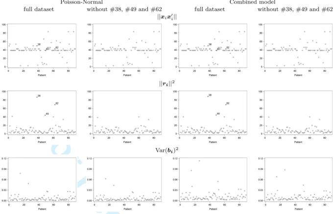
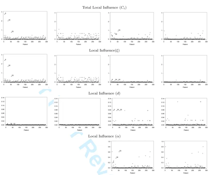
Parameter estimates are given in Table 1. Index plots (versus patient ID) for various local influence analyses are given in Figure 2. The top row of the plot represents the total local influence, with subsequent rows representing influence for sub-vectors: fixed

effects, random-intercept variance d, and, for the (PGN), the overdispersion parameter

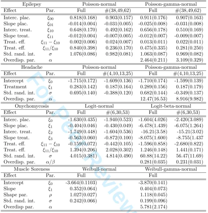
α, respectively. Patients #38, #49, and #62 stand out with large total influenceCi when

compared to other patients. Importantly, influences show a major drop when switching from (P-N) to (PGN). This is most prominently seen for #38. For an explanation, turn to the right hand panel of Figure 1. Patient #38 (and to some extent also #62 on the

1 2 3 4 5 6 7 8 9 10 11 12 13 14 15 16 17 18 19 20 21 22 23 24 25 26 27 28 29 30 31 32 33 34 35 36 37 38 39 40 41 42 43 44 45 46 47 48 49 50 51 52 53 54 55 56 57 58

(15)

For Peer Review Only

left hand side) alternates periodically between very high numbers of episodes and periods virtually without. This implies that their mean, variance, and association structure are rather different from the majority of subjects. The impact on the mean structure, by way of the fixed effects, is evident in the second row. For the (P-N) it is less clear when turning

tod, but we gain a lot of insight from the (PGN) results. Overall influence and influence

on ξ reduce drastically, but there now is clear influence on d and α. What it means

is that with these subjects present, the overdispersion parameter helps capturing their

anomalous behavior, which ‘deflates’ d. In other words, adding overdispersion protects

the inferentially crucial fixed-effects parameter vector. When removing these subjects, and also #49, little or no influence is left.

Note that the (PGN) model fitted to the full dataset exhibits a smaller value for α,

which corresponds to more overdispersion (no overdispersion corresponds to α

approach-ing +∞), while it does not vanish with removal of the three subjects. Thus, there appears to be genuine overdispersion in the data, further inflated by the influential subjects.

In agreement with Molenberghs, Verbeke, and Dem´etrio [20] and Molenberghs et al

[21], we consider the treatment effect in additive (ξ11−ξ01) and multiplicative (ξ11/ξ01)

form. Important differences are seen on the additive scale. (P-N) shows no significance

(p = 0.7106), which is sustained for (PGN), with p = 0.2225. Removing the influential

subjects leads to a highly significant result for (P-N), with p = 0.0009, which changes

to the still significant p = 0.0350 for (PGN). Hence, the influential subjects mask a

treatment effect. This is logical, because the influential subjects exhibit an oscillating behavior, introducing an important source of variability. At the multiplicative level, where

the null hypothesis is for the ratio to be 1, the story is nicely confirmed, with p= 0.6872

and p = 0.1166 for (P-N) and (PGN), respectively; the counterparts after deletion are

p <0.0001 andp= 0.0040, respectively.

To get further insight as to why these subject have higher influence than others, plots with interpretable components are given in Figure 3: ‘squared length of the fixed effects’ ||xix0i||, ‘squared length of the residual’ ||ri||2, and ‘random-effect variability’ Var(bi)2.

It is hardly surprising that #38 stands out in terms of||ri||2. Influences on #49 and #62

are less pronounced.

Our analysis has provided insight not available from earlier analysis. The influential subjects exhibit a cyclic behavior not observed in the majority of patients, but at the same time well documented. Based on these findings, a focused clinical discussion can take place, to determine the course of action. Options include removal, retention, or even setting up a dedicated study to further scrutinize this sub-population. In this case, a small group of patients with oscillating behavior between two poles has been identified.

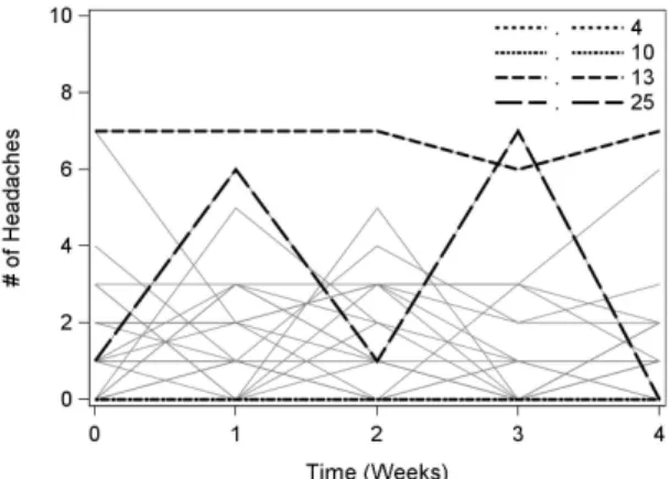
6.2 Headache Study

For these data, the model of Ouwens, Tan, and Berger [24] is used again:

E(Yij|ξ, bi) =tijexp(ξ0+Tijξ1+bi), (30)

whereTij indicates whether either placebo or Aspartame is given to patientiat occasion

j,bi∼N(0, d), andtij is the length of this period in days. We consider (P-N) and (PGN).

Figure S.4 in Supplementary Material shows the individual profiles. From this figure, and from some influence graphs in Figure S.5, patients #13, #25, #4, and #10 de-serve further investigation. The individual profiles show that the former two have more headaches than is typically the case; the latter two have none. Subjects #4 and #10 show

up in the total influence and that on d for the (P-N), while #13 is influential for the

fixed effects. No further influences are seen after removal of these four patients. Also, the

1 2 3 4 5 6 7 8 9 10 11 12 13 14 15 16 17 18 19 20 21 22 23 24 25 26 27 28 29 30 31 32 33 34 35 36 37 38 39 40 41 42 43 44 45 46 47 48 49 50 51 52 53 54 55 56 57 58

(16)

For Peer Review Only

relatively strong influences in (P-N) essentially disappear when turning to the (PGN). In other words, these influential subjects induce overdispersion which, when accommo-dated, strongly alleviates their influential status. Parameter estimates (standard errors) are reported in Table 1. While there is a borderline significant treatment effect in the

(P-N) fitted to all data (p= 0.0463), and a borderline non-significant one in the (PGN)

fitted to the full data (p = 0.0639), it disappears after removal (p = 0.2542 for (P-N)

and p= 0.2962 for (PGN)). This underscores that a few subjects might drive the alleged

treatment effect. Note that the effect of removal in terms of significance is opposite to that in the epilepsy study. The interpretable components do not lead to additional insight (Figures S.6 in Supplementary Material).

6.3 A Clinical Trial in Onychomycosis

Molenberghs et al [21] assumedYij|bi ∼Bernoulli(πij), where Yij is severity of infection

(1 for severe, 0 for non-severe) for patientiat occasionj,Tiis the treatment indicator (1

for experimental, 0 for standard) for subject, tj is the time point (months) at which the

jth measurement has been taken, and bi ∼N(0, d). The conditional success probability

is expressed as:

logit(πij) =ξ1(1−Ti) +ξ2(1−Ti)tij +ξ3Ti+ξ4Titij+bi.

Both the logit-normal (L-N) and logit-beta-normal (LBN) are fitted. Parameter esti-mates (standard errors) are displayed in Table 1, with local influence plots in Figure S.7 (in Supplementary Material). Subjects #6, #30, and #53 are detected as influential, overall, and with respect to the fixed effects, in the (L-N). Accommodating overdisper-sion, hence turning to the (LBN), deflates the magnitude of influence. Likewise, influence is drastically diminished by removing these three subjects. Thus, in case the influential subjects should remain in the analysis, the (LBN) may be the most sensible route for-ward. Alternatively, in case they are considered anomalous, one can remove them. To decide on which scenario is preferred in this case, we note that all three subjects are unusual: they set out with a sequence of non-severe ratings, but then switch to a severe rating (‘0000111’ for #6, ‘0000011’ for #30, and ‘0000001’ for #53). Arguably, there is no reason to remove these subjects from analysis, partly also to safeguard randomization. However, it is uncommon to switch from non-severe to severe in this particular way, so these patients must be further clinically scrutinized. Also for these data, the interpretable components do not lead to further insight (Figure S.8 in Supplementary Materials).

The (L-N) and (LBN) lead to borderline significance when applied to the full data

[p = 0.0268 additively andp = 0.0560 multiplicatively for (L-N); p = 0.0627 additively

and p = 0.0964 multiplicatively for (LBN)]. When influential subjects are removed,

these values all become highly significant [in the same order, p < 0.0001, p = 0.0007,

p = 0.0011, and p = 0.0099]. These findings are qualitatevely similar to the epilepsy

cases, but different from the headache study.

6.4 Recurrent Muscle Soreness

The Weibull-normal (W-N) and Weibull-gamma-normal (WGN) models are considered,

with scale parameter λ = 1, and linear predictor ηij = ξ0 +bi+ξ1Ti, where Ti is an

indicator for treatment and bi ∼ N(0, d). Parameter estimates (standard errors) are in

Table 1. Local influence plots and interpretable components are displayed in Figures S.9 and S.10 in Supplementary Materials, respectively. Unlike in the three previous studies, no subjects stand out. It is clear though, that influence goes down when turning from

1 2 3 4 5 6 7 8 9 10 11 12 13 14 15 16 17 18 19 20 21 22 23 24 25 26 27 28 29 30 31 32 33 34 35 36 37 38 39 40 41 42 43 44 45 46 47 48 49 50 51 52 53 54 55 56 57 58

(17)

For Peer Review Only

the (W-N) to the (WGN). It is equally important to see no influence is detected when there happens to be none.

7. Simulation Study

In order to evaluate the relative performance of local influence in the context of the two different models, standard and combined, a small-scale simulation study was conducted. To define realistic simulation scenarios, the various standard models were considered, for the epilepsy data, the onychomycosis data, and the recurrent muscle soreness data, respectively (see Table 1). These parameter estimates were then used as true values in the simulations and plugged into the corresponding model for each of the three data types. This model is then used to generate the response variables Ynew

ij . Various sets

of covariate values from the original dataset were considered; they were kept fixed across simulation runs. Some predetermined influential subjects are chosen prior to the simulation study for each situation. We consider three types of predetermined influential subjects: high, medium, and low. The local influence analysis is run for each simulated dataset. A cut-off value for local influence is defined as 2PN

i=1Ci/N [17]. Every time, 200 replicated datasets

were generated.

The simulation results are presented in Tables 2–4. Table 2 shows the sum-mary statistics. While convergence was unproblematic in the count and time-to-event cases, more difficulties were encountered in the binary case: the com-bined model gave valid result only for 145 simulations. It is known that iden-tifying overdispersion on top of data correlation in the binary case is harder. From this table, it can be seen that the combined model for all data types identified the influential subjects more frequently than the standard GLMM. Observe that the mean of the local influence values for the combined models are lower than those from the GLMM (Table 3). These findings are in line with the analysis from the original datasets, showing that the local influence for combined models are lower than those from the GLMM.

A classification of the predetermined influential subjects is given in Ta-ble 4. Most of the highly influential subjects are classified as influential, for both models and all three data types. In contrast, medium- and low-influence subjects are not always recognized.

8. Concluding Remarks

Local influence was studied before as a means to detect outlying subjects, and features thereof, for the linear mixed model and some generalized linear mixed models. We have extended this work in several ways. First, local influence measures are derived for several GLMM: Poisson-normal, logit-normal, probit-normal, and Weibull-normal. Second, also for the extensions of these model that capture overdispersion, i.e., the combined model, influence measures are derived. Third, using the integral form of the log-likelihood, it has been possible to derive interpretable components of influence, like for the LMM, but un-like in earlier influence work for the GLMM. Beyond identifying influential subjects, this allows us to scrutinize which aspects leads to influence on important model parameters and conclusions based there upon.

In all four case studies analyzed, it is seen that accounting for overdispersion allevi-ates influence, whether for a few outlying subjects or for the dataset as a whole. When

1 2 3 4 5 6 7 8 9 10 11 12 13 14 15 16 17 18 19 20 21 22 23 24 25 26 27 28 29 30 31 32 33 34 35 36 37 38 39 40 41 42 43 44 45 46 47 48 49 50 51 52 53 54 55 56 57 58

(18)

For Peer Review Only

there are outlying subjects in the GLMM, it is often seen that removing them leads to reductions similar to switching to the combined model. Of course, these actions are very different and depend on whether one wants to either homogenize the original data or, conversely, retain these subjects for analysis, but then change the model to one that allows for this without undue influence. The combined model is a good candidate for this. This is underscored by the fact that treatment effect assessment can change in different ways upon removing influential subjects. In the epilepsy and onychomycosis studies, treatment effect turns from non- to (highly) significant; in the headache study, a borderline significant effect disappears after removing influential subjects.

Evidently, beyond the distributions considered here, others could be studied as well. For example, with time-to-event data, it is not uncommon to use log-normal rather than Weibull distributions. Our method is generic and has been applied to a collection of distributions; similar calculations would lead to expressions for alternative distributions. Web Appendices S.1–S.6, referenced in Section 5, are available in conjunction with this paper.

The methodology developed here has been implemented in the SAS soft-ware system. Fitting the models is done using the SAS procedure NLMIXED and macros have been developed for the local influence calculations. The codes are available in the Supplementary Materials.

Acknowledgments

Financial support from the IAP research network #P7/06 of the Belgian Government (Belgian Science Policy) is gratefully acknowledged.

References

[1] Beckman, R.J., Nachtsheim, C.J., and Cook, R.D. (1987) Diagnostics for mixed-model analysis of

variance.Technometrics,29, 413–426.

[2] Breslow, N.E. and Clayton, D.G. (1993) Approximate inference in generalized linear mixed models. Journal of the American Statistical Association,88, 9–25.

[3] Chatterjee, S. and Hadi, A.S. (1988) Sensitivity Analysis in Linear Regression. New York: John

Wiley & Sons.

[4] Chen, X.-D., Fu, Y.-Z., and Wang, X.-R. (2013) Local influence measure of zero-inflated generalized

Poisson mixture regression models.Statistics in Medicine,32, 1294–1312.

[5] Cook, R.D. (1977a) Detection of influential observations in linear regression. Technometrics,19,

15–18.

[6] Cook, R.D. (1977b) Letter to the editor.Technometrics,19, 348.

[7] Cook, R.D. (1979) Influential observations in linear regression.Journal of the American Statistical

Association,74, 169–174.

[8] Cook, R.D. (1986) Assessment of local influence.Journal of the Royal Statistical Society, Series B,

48, 133–169.

[9] Cook, R.D. and Weisberg, S. (1982) Residuals and Influence in Regression. London: Chapman &

Hall.

[10] De Backer, M., De Keyser, P., De Vroey, C., and Lesaffre, E. (1996) A 12-week treatment for dermatophyte toe onychomycosis: terbinafine 250mg/day vs. itraconazole 200mg/day–a double-blind

comparative trial.British Journal of Dermatology134, 16–17.

[11] Engel, B. and Keen, A. (1994) A simple approach for the analysis of generalized linear mixed models. Statistica Neerlandica,48, 1–22.

[12] Faught, E., Wilder, B.J., Ramsay, R.E., Reife, R.A., Kramer, L.D., Pledger, G.W., and Karim, R.M. (1996) Topiramate placebo-controlled dose-ranging trial in refractory partial epilepsy using 200-,

400-, and 600-mg daily dosages,Neurology,46, 1684–1690.

[13] Golub, G.H. and Van Loan, C.F. (1989) Matrix Computations. (2nd ed.). Baltimore: The Johns

Hopkins University Press.

1 2 3 4 5 6 7 8 9 10 11 12 13 14 15 16 17 18 19 20 21 22 23 24 25 26 27 28 29 30 31 32 33 34 35 36 37 38 39 40 41 42 43 44 45 46 47 48 49 50 51 52 53 54 55 56 57 58

(19)

For Peer Review Only

[14] Hosmer, D.W. and Lemeshow, S. (1999) Applied Survival Analysis: Regression Modelling of Time

to Event Data. Chichester: John Wiley & Sons.

[15] Jansen, I., Molenberghs, G., Aerts, M., Thijs, H., and Van Steen, K. (2003) A Local influence

approach applied to binary data from a psychiatric study.Biometrics,59, 410–419.

[16] Johnson, N.L. and Kotz, S. (1970)Distributions in Statistics, Continuous Univariate Distributions,

Vol. 2.Boston: Houghton-Mifflin.

[17] Lesaffre, E. and Verbeke, G. (1998) Local influence in linear mixed models.Biometrics,54, 570–582.

[18] McKnight, B. and Van Den Eeden, S.K. (1993) A conditional analysis for two-treatment multiple

period crossover designs with binomial or Poisson outcomes and subjects who drop out.Statistics

in Medicine,12, 825–834.

[19] Molenberghs, G. and Verbeke, G. (2005)Models for Discrete Longitudinal Data.New York: Springer.

[20] Molenberghs, G., Verbeke, G., and Dem´etrio, C. (2007) An extended random-effects approach to

modeling repeated, overdispersed count data.Lifetime Data Analysis,13, 513–531.

[21] Molenberghs, G., Verbeke, G., Dem´etrio, C.G.B., and Vieira, A. (2010). A family of generalized

linear models for repeated measures with normal and conjugate random effects.Statistical Science,

25, 325–347.

[22] Mun, J. and Lindstrom, M.J. (2013) Diagnostics for repeated measurements in linear mixed effects

models.Statistics in Medicine,32, 1361–1375.

[23] Neter, J., Wasserman, W., and Kutner, M.H. (1990)Applied Linear Statistical Models. Regression,

Analysis of Variance and Experimental Designs(3rd ed.). Homewood, IL: Richard D. Irwin, Inc. [24] Ouwens, M.J.N.M., Tan, F.E.S., and Berger, M.P.F. (2001). Local influence to detect influential

data structures for generalized linear mixed models.Biometrics,57, 1166–1172.

[25] Roberts, D.T. (1992) Prevalence of dermatophyte onychomycosis in the United Kingdom: results of

an omnibus survey.British Journal of Dermatology,126, 23–27.

[26] Verbeke, G. and Molenberghs, G. (2000) Linear Mixed Models for Longitudinal Data. New York:

Springer-Verlag.

[27] Verbeke, G., Molenberghs, G., Thijs, H., Lesaffre, E., and Kenward, M.G. (2001) Sensitivity analysis

for non-random dropout: a local influence approach.Biometrics,57, 7–14.

[28] Wolfinger, R. and O’Connell, M. (1993) Generalized linear mixed models: a pseudo-likelihood

ap-proach.Journal of Statistical Computation and Simulation,48, 233–243.

[29] Zeger, S.C., Liang, K.-Y., and Albert, P.S. (1988) Models for longitudinal data: a generalized

esti-mating equation approach.Biometrics,44, 1049–1060.

[30] Zhu, H. and Lee, S. (2001). Local influence for incomplete-data models.Journal of the Royal

Sta-tistical Society, Series B (StaSta-tistical Methodology),63, 111–126.

[31] Zhu, H., Lee, S., Wei, B.-C., and Zhou, J. (2001). Case-deletion measures for models with incomplete

data.Biometrika,88, 727–737. 1 2 3 4 5 6 7 8 9 10 11 12 13 14 15 16 17 18 19 20 21 22 23 24 25 26 27 28 29 30 31 32 33 34 35 36 37 38 39 40 41 42 43 44 45 46 47 48 49 50 51 52 53 54 55 56 57 58

(20)

For Peer Review Only

Table 1. Parameter estimates (standard errors) for the generalized linear mixed and combined models.

Epilepsy Poisson-normal Poisson-gamma-normal

Effect Par. Full #(38,49,62) Full #(38,49,62)

Interc. plac. ξ00 0.818(0.168) 0.903(0.157) 0.911(0.176) 0.907(0.163) Slope plac. ξ01 -0.014(0.004) -0.031(0.005) -0.025(0.008) -0.031(0.008) Interc. treat. ξ10 0.648(0.170) 0.492(0.162) 0.656(0.178) 0.510(0.169) Slope treat. ξ11 -0.012(0.004) -0.007(0.005) -0.012(0.007) -0.009(0.007) Treat. eff. ξ11−ξ10 0.002(0.006) 0.024(0.007) 0.013(0.011) 0.022(0.011) Treat. eff. ξ11/ξ10 0.840(0.398) 0.236(0.170) 0.475(0.335) 0.281(0.250) Std. rand. int. σ 1.076(0.086) 0.982(0.081) 1.063(0.087) 0.969(0.082) Overdisp. par. α 2.464(0.211) 3.109(0.329)

Headache Poisson-normal Poisson-gamma-normal

Effect Par. Full #(4,10,13,25) Full #(4,10,13,25)

Intercept ξ0 -1.715(0.172) -1.609(0.136) -1.710(0.174) -1.599(0.139)

Treatment ξ1 0.283(0.142) 0.187(0.164) 0.289(0.156) 0.187(0.179)

Std. rand. int. σ 0.695(0.140) -0.388(0.120) 0.682(0.144) -0.349(0.137)

Overdisp. par. α 12.47(16.53) 8.916(9.982)

Onychomycosis Logit-normal Logit-beta-normal

Effect Par. Full #(6,30,53) Full #(6,30,53)

Interc. plac. ξ0 -1.630(0.435) -1.940(0.523) -1.604(4.026) -2.420(3.089) Slope plac. ξ1 -0.404(0.046) -0.430(0.049) -6.478(1.439) -6.075(1.264) Interc. treat. ξ2 -1.749(0.448) -1.604(0.536) -16.21(3.58) -15.21(3.02) Slope treat. ξ3 -0.563(0.060) -0.872(0.100) -8.075(1.600) -8.755(1.437 Treat. eff. ξ11−ξ10 -0.159(0.072) -0.442(0.105) -1.596(0.858) -2.680(0.822) Treat. eff. ξ11/ξ10 1.394(0.206) 2.028(0.302) 1.246(0.148) 1.441(0.171) Std. rand. int. σ 4.015(0.381) 4.814(0.490) 60.88(14.22) 56.47(11.69) Overdisp. par. α/β 0.281(0.035) 0.231(0.031)

Muscle Soreness Weibull-normal Weibull-gamma-normal

Effect Par. Full Full

Intercept ξ0 -3.664(0.1103) -3.870(0.141) Slope ξ1 0.352(0.064) 0.404(0.073) Shape par. ρ 1.027(0.027) 1.118(0.045) Std. rand. int. σ 0.242(0.066) 0.199(0.096) Overdisp par. α 5.781(2.174) 1 2 3 4 5 6 7 8 9 10 11 12 13 14 15 16 17 18 19 20 21 22 23 24 25 26 27 28 29 30 31 32 33 34 35 36 37 38 39 40 41 42 43 44 45 46 47 48 49 50 51 52 53 54 55 56 57 58

(21)

For Peer Review Only

Table 2. Simulation study. The mean for total number of influence subjects across all simulations.

Source Mean Std. Dev. Mean Std. Dev.

Total Local Influence (Ci) 6.630 1.122 8.180 0.890

Local Influence(ξ) 6.630 1.067 7.250 0.928

Local Influence (d) 9.220 1.371 8.885 1.048

Local Influence (α) 6.035 1.009

Local Influence(ρ) 40.28 4.152 42.165 3.764

Table 3. Simulation study. The mean of local influence across all simulations.

Source Mean Std. Dev. Mean Std. Dev.

Local Influence(ξ) 0.090 0.006 0.010 0.00001 Local Influence(ρ) 0.034 0.002 0.005 0.00015 Local Influence (d) 0.940 0.050 0.006 0.001 Local Influence (α) 0.003 0.009 1 2 3 4 5 6 7 8 9 10 11 12 13 14 15 16 17 18 19 20 21 22 23 24 25 26 27 28 29 30 31 32 33 34 35 36 37 38 39 40 41 42 43 44 45 46 47 48 49 50 51 52 53 54 55 56 57 58

(22)

For Peer Review Only

Table 4. Simulation study. Classification of predetermined influential subjects across all simulations.

Category Subject Not Influential Influential Not Influential Influential

High #5 0 200 0 200 #38 1 199 0 200 #49 0 200 0 200 #62 0 200 0 200 Medium #2 174 26 1 199 #16 200 0 200 0 #60 173 27 151 49 #73 0 200 0 200 Low #11 200 0 145 55 #39 200 0 200 0 #63 23 177 12 188 #67 200 0 200 0

High #6 0 200 1 139 #30 0 200 1 144 #53 0 200 1 144 #198 0 200 2 143 Medium #3 0 200 1 143 #13 0 200 2 142 #276 0 200 2 139 #279 0 200 1 143 Low #244 94 106 139 1 #257 94 106 139 1 #272 152 48 136 1 #290 152 48 136 1

High #62 7 193 0 200 #169 27 173 0 200 #328 0 200 0 200 #378 0 200 0 200 Medium #31 200 0 0 200 #64 200 0 0 200 #259 0 200 0 200 #317 0 200 0 200 Low #30 200 0 198 2 #161 200 0 175 25 #237 0 200 0 200 #299 0 200 0 200 1 2 3 4 5 6 7 8 9 10 11 12 13 14 15 16 17 18 19 20 21 22 23 24 25 26 27 28 29 30 31 32 33 34 35 36 37 38 39 40 41 42 43 44 45 46 47 48 49 50 51 52 53 54 55 56 57 58

(23)

For Peer Review Only

Figure 1. Epilepsy Data. Individual profiles.

Poisson-normal Poisson-gamma-normal

full dataset without #38, #49 and #62 full dataset without #38, #49 and #62

Total Local Influence (Ci)

Local Influence(ξ)

Local Influence (d)

Local Influence (α)

Figure 2. Epilepsy Data. Local influence plots. 1 2 3 4 5 6 7 8 9 10 11 12 13 14 15 16 17 18 19 20 21 22 23 24 25 26 27 28 29 30 31 32 33 34 35 36 37 38 39 40 41 42 43 44 45 46 47 48 49 50 51 52 53 54 55 56 57 58

(24)

For Peer Review Only

Poisson-Normal Combined model

full dataset without #38, #49 and #62 full dataset without #38, #49 and #62

||xix0i||

||ri||2

Var(bi)2

Figure 3. Epilepsy Data. Plots of interpretable components of local influence. 1 2 3 4 5 6 7 8 9 10 11 12 13 14 15 16 17 18 19 20 21 22 23 24 25 26 27 28 29 30 31 32 33 34 35 36 37 38 39 40 41 42 43 44 45 46 47 48 49 50 51 52 53 54 55 56 57 58

(25)

For Peer Review Only

SUPPLEMENTARY MATERIALS

Local Influence Diagnostics for Generalized Linear Mixed

Models With Overdispersion

Trias Wahyuni Rakhmawatia Geert Molenberghsa,b Geert Verbekeb,a Christel Faesa,b

[email protected]

a_{I-BioStat, Universiteit Hasselt, B-3500 Hasselt, Belgium} b_{I-BioStat, Katholieke Universiteit Leuven, B-3000 Leuven, Belgium}

S.1. Expressions for Standard Local Influence: Subsets

When only a subsetθ1 ofθ= (θ01,θ02)0 is of special interest, the methodology still applies.

it follows that (Verbeke and Molenberghs 2000) the corresponding influence:

Ch(θ1) =Ch + 2h0∆0 0 0 0 ¨L−₂₂1 ∆h≤Ch, (S.1.1)

with obvious notation. Should ¨L12= 0, then an influence decomposition is possible:

Ch =Ch(θ1) + Ch(θ2). (S.1.2)

For weakly correlated sub-vectors, (S.1.2) holds approximately.

S.2. Local Influence for the Linear Mixed Model

S.2.1 Standard Approach, Based on the Marginal Likelihood

The backdrop for our developments is the method as derived for the linear mixed model (Verbeke and Lesaffre 1997b, Verbeke and Molenberghs 2000). We will sketch their de-velopments, and then turn to an alternative derivation based on the likelihood in integral form.

In line with these authors, we consider (4), but with in addition the conditional

inde-pendence assumption Σi =σ2Ini, withIni theni×ni identity matrix.

For Ci as in (21), a convenient form can be derived:

Ci =−2

ˆ

θ−θˆ1₍_i₎0L¨₍_i₎L¨−1L¨₍_i₎θˆ−θˆ1₍_i₎, (S.2.1)

where a subscript (i) indicates that the corresponding quantity is based on the deletion of

theith subject and further the vectorθˆ1₍_i₎ is the one-step approximation toθˆ₍_i₎obtained

from a single Newton-Raphson step in the maximization procedure of`(i)(θ), using θˆas

the starting value. For sufficiently large sample size, it follows thatCiis an approximation

1 2 3 4 5 6 7 8 9 10 11 12 13 14 15 16 17 18 19 20 21 22 23 24 25 26 27 28 29 30 31 32 33 34 35 36 37 38 39 40 41 42 43 44 45 46 47 48 49 50 51 52 53 54 55 56 57 58

(26)

For Peer Review Only

to the classical global case-deletion diagnostics. Note that the expression is exact when properly used for local influence purposes.

It is advantageous that Ci admits a closed form (21). Lesaffre and Verbeke (1998)

decomposed Ci into five interpretable components. Let Ri, Xi, and Zi denote now the

“standardized” residuals and covariates for the ith individual, defined byR_i =V_i−1/2ri,

X_i =V_i−1/2Xi, andZi =V

−1/2

i Zi, respectively, withri =yi−Xiβb. Further, for a matrix

A, let kAk =ptr(A0A) be the Frobenius norm of A (Golub and Van Loan 1989). The

interpretable components in Ci are then

kX_iX_i0k, kR_ik, kZ_iZ_i0k, kI −R_iR_i0k, kV_i−1k. (S.2.2)

First,kXiXi0kmeasures the “length” of the standardized covariates in the mean structure

and kR_ik is an overall measure for how well the observed data for the ith subject are

predicted by the mean structureXiβ. Second, the componentskZiZi0kandkI−RiRi0k

have a similar meaning, but then for the covariance structure. For example,kI−R_iR_i0k

will be zero only if Vi equals riri0. Note that riri0 is an estimate for var(yi), which

only assumes the mean to be correctly modeled as Xiβ. Therefore, kI −RiRi0k can

be interpreted as a residual, capturing how well the covariance structure of the data is

modeled by Vi = ZiDZ_i0 +σ2Ini. Finally, the fifth component kV

−1

i k will be large if

Vi has small eigenvalues, which indicates that the ith subject is assumed to have small

variability.

The decomposition of Ci immediately suggests a practical procedure to find an

expla-nation for the influential nature of an individual, i.e., when Ci is large, we examine the

diagnostics. Such plots are useful to graphically inspect the individuals in view of their

influential nature. Thus, it is sensible to start with an index plot ofCi. Following this, the

index plots of (??) can be examined. A recurrent practical difficulty with diagnostics is

to establish a threshold above which an individual is defined as “remarkable”. It follows from (21) that N X i=1 Ci=−2 tr L¨−1 N X i=1 ∆i∆0i ! ,

which converges to 2s, for N approaching infinity. As for leverage in linear regression

(Neter, Wasserman and Kutner 1990, pp. 395–396), one could classify an individual for

which Ci is larger than twice the average value (larger than 4s/N, forN large) as being

influential. However, unlike for the leverage situation, 2s is only the approximate sum

of the Ci, which will not be accurate if the model is not correctly specified (such that

¨

L−1P

i∆i∆

0

i does not converge to Is) or if N is too small for the asymptotic results

to yield good approximations. In such cases, Lesaffre and Verbeke (1998) proposed to

replace 2s by the actual sum, and we call theith subject influential if Ci is larger than

the cutoff value 2PN

i=1Ci/N.

Given decomposition result (S.1.1), it is interesting to consider sub-vectors β and

α of fixed effects and variance components, respectively, with corresponding influences

Ci(β) andCi(α), respectively. Given that the fixed effects and variance components are

asymptotically independent, it follows that

Ci≈Ci(β) + Ci(α). (S.2.3)

Lesaffre and Verbeke (1998) further showed that Ci(β) can be decomposed using only

the first two components kXiXi0k and kRik, while the last three components kZiZi0k,

1 2 3 4 5 6 7 8 9 10 11 12 13 14 15 16 17 18 19 20 21 22 23 24 25 26 27 28 29 30 31 32 33 34 35 36 37 38 39 40 41 42 43 44 45 46 47 48 49 50 51 52 53 54 55 56 57 58

(27)

For Peer Review Only

kI−RiRi0k, andkVi−1kfeature in the decomposition ofCi(α). Asymptotically therefore,

influence for the fixed effects and for the variance components can be scrutinized by studying the first two and the last three interpretable components, respectively.

S.2.2 Integral-based Expression

As previewed in Section 4, the integral-based approach is used here as an alternative way to alleviate complexities with the explicit marginal likelihood expressions. To prepare for developments of Poisson, probit, logit and Weibull cases, we set out this way for the linear mixed model.

The marginal density corresponding to the linear mixed model is defined by the fol-lowing expression: e f(y_i) = Z e f(y_i|β,bi)fe(b_i|D) db_i. (S.2.4)

The conditional density of the response variable takes the form:

e f(y_i|β,bi) = 1 2πσ2 ni/2 exp − 1 2σ2(yi−Xiβ−Zibi) 0₍_y i−Xiβ−Zibi) = (2πs)−ni/2_exp[_f₍_y i)], (S.2.5) wheref(y_i) =−(2s)−1(y_i−y_b_i)0(y_i−y_b_i) ;ybi=Xiβ+Zibi, ands=σ 2_{. The conditional}

density of the normal random effect is:

f(bi) = 1 (2π)q/2_|_D_|1/2 exp −1 2bi 0 D−1bi = 2π−q/2|D|−1/2exp{g(bi)}, (S.2.6)

where g(bi) =−1₂bi0D−1bi.Thus, the marginal density for the linear mixed model is:

e

f(y_i) = (2π)−(ni+q)/2_s−ni/2_|_D_|−1/2

Z

exp{f(y_i) +g(bi)}dbi. (S.2.7)

From (S.2.7) the likelihood derives as:

L(β, D, s) = N Y i=1 e f(y_i), (S.2.8)

and the corresponding log-likelihood is (18). Thus, the log-likelihood contribution of the

1 2 3 4 5 6 7 8 9 10 11 12 13 14 15 16 17 18 19 20 21 22 23 24 25 26 27 28 29 30 31 32 33 34 35 36 37 38 39 40 41 42 43 44 45 46 47 48 49 50 51 52 53 54 55 56 57 58

(28)

For Peer Review Only

ith individual takes the form:

`i(β, D, s) = log (2π)−(ni+q)/2_s−ni/2_|_D_|−1/2 Z exp{f(y_i) +g(bi)}dbi =−(ni+q) 2 log(2π)− ni 2 log(s)− 1 2log|D| + log Z exp[f(y_i) +g(bi)]dbi ∝ −ni 2 log(s)− 1 2log|D|+ logKi, (S.2.9) where Ki= R Iidbi and Ii = exp{f(yi) +g(bi)}.

To derive the local influence as described in (21), the components of local influence

need to be derived. Lesaffre and Verbeke (1998) showed that Ci equals:

Ci = 2||L¨−1|| ||∆i||2cos(ϕi), (S.2.10)

where ϕi is the angle between vec(−L¨−1) and vec(∆i∆0i), ∆i is the first derivative of

`i(β, D, s) with respect to the model parameters, and ¨L−1 is the s×smatrix of second

derivatives of `(β, D, s) with respect to the parameters.

The procedure to construct derivatives with respect to the parameters is as follows.

First, the derivative with respect to fixed effect β is:

∂`i(β, D, s) ∂β = 1 Ki Z Ii 1 sXi 0₍_y i−yˆi)dbi= 1 sXi 0Li Ki , (S.2.11) where Ki = Z Iidbi = Z exp[f(y_i) +g(bi)]dbi=cφe(y_i) (S.2.12) and Li= Z Ii(yi−ybi)dbi = Z Ii(yi−Xiβ−Zibi)dbi =y_i Z Iidbi−Xiβ Z Iidbi−Zi Z Iibidbi. (S.2.13) 1 2 3 4 5 6 7 8 9 10 11 12 13 14 15 16 17 18 19 20 21 22 23 24 25 26 27 28 29 30 31 32 33 34 35 36 37 38 39 40 41 42 43 44 45 46 47 48 49 50 51 52 53 54 55 56 57 58

(29)

For Peer Review Only

Component RIibidbi of Li can be rewritten as:

Z Iibidbi = Z cφe(y_i,b_i)b_idb_i =c Z e φ(y_i)φe(b_i|y_i)b_idb_i =cφe(y_i) Z biφe(b_i|y_i)db_i =cφe(y_i)E(b_i|y_i) =cφe(y_i)DZ0_iV−_i 1(y_i−X_iβ) =cφe(y_i)DZ0_iV−_i 1r_i, (S.2.14)

where ri =yi−Xiβ. Expanding the component functions of (S.2.11) leads to:

∂`i(β, D, s) ∂β = 1 sXi 0Li Ki = 1 sXi 0 y_i−Xiβ−ZiDZ0iV −1 i (yi−Xiβ) = 1 sXi 0 (Ini−ZiDZ0iV −1 i )(yi−Xiβ) = 1 sXi 0 (s+ZiDZ0i)V −1 i −ZiDZ 0 iV −1 i (yi−Xiβ) = 1 sXi 0_s_V−1 i (yi−Xiβ) =Xi0V−i 1ri. (S.2.15)

Second, the derivative with respect to s≡σ2 is as follows:

∂`i(β, D, s) ∂s =− ni 2s+ 1 Ki Z Ii 1 2s2(yi−ybi) 0₍_y i−ybi)dbi =−ni 2s− 1 sKi Z Iif(yi)dbi =−1 s ni 2 + 1 Ki Z Iif(yi)dbi , (S.2.16) 1 2 3 4 5 6 7 8 9 10 11 12 13 14 15 16 17 18 19 20 21 22 23 24 25 26 27 28 29 30 31 32 33 34 35 36 37 38 39 40 41