Tradeoff Studies about Storage and Retrieval Efficiency of Boundary Data
Representations for LLS, TIGER and DLG Data Structures
1
Introduction
Boundary information is viewed as an efficient representation of image documents describing spatial regions and is important for document image management and information retrieval. Boundary information represents one type of vector information [1, Chapter 15]. Boundaries (or contours or outlines) are mathematically described as convex or non-convex polygons. One boundary can be formed by a set of polygons, for instance, a donut shape boundary. Each polygon consists of an ordered set of points or vertices. In most GIS applications, points are georeferenced so that boundary information can be integrated with raster information. GIS examples of boundary information would be parcels, eco-regions, watersheds, soil regions, counties, Census tracts or U.S. postal zip codes. The goal of our work is to study the impacts of choosing boundary information representation on document image management and informational retrieval, as well as improve our understanding of the processing noise introduced during representation conversions.
In general, boundaries can be spatially related or can be spatially independent. The spatially related boundaries can be either partially overlapping or totally overlapping, such as, one contour being a subset of another set of boundaries. For example, watershed and U.S. postal zip codes boundaries are spatially independent while the U.S. Census Bureau tracts and blocks are spatially dependent in such a way that every tract is formed by a set of blocks.
Given the variety of boundary information, researchers have developed numerous file formats for storing boundary information. These file formats are designated in general for storing any vector data. Vector data contain points, lines, arcs, polygons or any combinations of these elements. Any vector data element can be represented in a reference domain defined by a latitude/longitude, UTM or pixel
David Clutter
Peter Bajcsy
National Center for Supercomputing
Applications (NCSA), University of Illinois at
Urbana-Champaign (UIUC)
605 East Springfield Avenue, Champaign, IL
61820
Abstract
We present our theoretical comparisons and experimental evaluations of three boundary data representations in terms of storage and information retrieval efficiency. We focus on three boundary data representations, such as, location list data structure (LLS), digital line graphs (DLGs) and topologically integrated geographic encoding and referencing (TIGER) data organizations. These three boundary data representations are used frequently in the GIS domain, and are known as ESRI Shapefiles (LLS), the SSURGO DLG-3 soil files (DLG), and the U.S. Census Bureau 2000 TIGER/Line files (TIGER). Boundary information is viewed as an efficient representation of image documents describing spatial regions. The goal of our work is to study the impacts of choosing boundary information representation on document image management and information retrieval, as well as to improve our understanding of the processing noise introduced during representation conversions.
Our storage and retrieval efficiency tradeoff evaluations are based on load time, computer memory, and hard disk space requirements. The experimental measurements are obtained with test data sets derived from the SSURGO DLG-3 soil files and the U.S. Census Bureau 2000 TIGER/Line files. Based on our experiments, we concluded that LLS files will provide the fastest boundary retrieval (40 times faster than TIGER and 2.5 times faster than DLG) at the price of file size (storage redundancy for LLS files is between 70% and 180% in our experiments). DLG format offers a smaller file size, but is less efficient for boundary retrieval. TIGER format also offers a compact physical representation, at the cost of more processing for boundary retrievals. These findings provide quantitative support for institutional document image management decisions.
coordinate system. The challenge in storing vector data is to organize the data such that the positions and geographic meanings of vector data elements are efficiently stored and easily extracted.
Among all vector data representations in files, the following data structures have been used frequently: location list data structure (LLS), point dictionary structure (PDS), dual independent map encoding structure (DIME), chain file structure (CFS), digital line graphs (DLGs) and topologically integrated geographic encoding and referencing (TIGER) files. For detailed description of each data structure we refer a reader to [1].
The motivation of our work came from the fact that while boundary data types are preferred over raster data types when it comes to storing boundary information, there are multiple memory storage schemes for boundary information, as listed in the previous paragraph. However, choosing the storage scheme that minimizes memory requirements might have a detrimental impact on boundary information retrieval efficiency. Thus, our objective is to evaluate quantitatively the tradeoffs between storage and retrieval efficiency of multiple boundary data representations for LLS, TIGER and DLG data structures. The outcomes of our evaluations are useful for (a) institutional decisions about archiving and retrieving geospatial boundary information, and (b) custom applications that perform processing of large size, geospatial boundary data sets.
In this work, we evaluate three boundary data representations for efficient boundary information storage and retrieval. These three data representations include (1) Census 2000 TIGER/Line files defined by the U.S. Census Bureau and saved in topologically integrated geographic encoding and referencing (TIGER) data structures, (2) shapefiles defined by the Environmental Systems Research Institute (ESRI) and stored in location list data structure (LLS) data structures, and (3) SSURGO DLG-3 soil boundaries prepared by the United States Geological Survey (USGS) and stored in digital line graphs (DLGs) data structures. We overview the three data file formats first. Next, we present our experimental results, and pair-wise analysis of experimental results. Finally, we summarize our work and add a few observations about other possible trade-off metrics that might be considered for making institutional decisions.
2
SSURGO DLG-3 Soil Files
The Soil Survey Geographic (SSURGO) Digital Line Graphs (DLG) files provide geographical information on the boundaries of soil types [9], [10], [11]. The SSURGO data sets provide the highest spatial resolution of soil type information among the three soil
geographic data bases, such as, the Soil Survey Geographic (SSURGO) data base, the State Soil Geographic (STATSGO) data base, and the National Soil Geographic (NATSGO) data base.
2.1
File Format Description
DLG File Structure: The DLG file structure is designed to support all categories of spatial data that can be represented on a map. Three distinct types of DLG are defined. Large-scale DLG data is digitized from 1:24,000-scale USGS topographic quadrangles (SSURGO). Intermediate-scale DLG data is digitized from 1:100,000-scale USGS quadrangles (STATSGO). Small-scale DLG data is digitized from 1:2,000,000-scale sectional maps (NATSGO). Furthermore, three levels of DLG data were defined in terms of the number of attributes. It was found that the widest user community would be served by DLG Level 3 (DLG-3) data, which allows for the highest resolution (SSURGO) and highest number of attributes to be encoded (Level 3). The lesser levels of DLG encoding are unused. DLG-3 encodes attributes using two codes: a major code and a minor code. Similar attributes share a major code. The SSURGO DLG-3 soil database uses both the major code and minor code to encode the primary key into a relational database to further describe an area.
We gathered the SSURGO DLG-3 files for a few
counties in Illinois from
http://www.ncgc.nrcs.usda.gov/branch/ssb/products/ ssurgo/data/index.html. There are two files for each county, such as, dlg.zip (digital line graph or DLG) and tab.zip (ASCII attribute data available in Microsoft Access 97 or later template database). The files contain soil boundaries of 18,000 soil series recognized in the United States. For the integration purposes, we have explored the following information from the DLG-3 documentation: (a) file naming convention, (b) spatial resolution, (c) spatial accuracy, (d) geographic coordinate system and (e) storage format. In terms of file naming convention, the dlg.zip file would contain files with the following suffixes:
af - soil polygon DLG-3 file, aa - soil polygon attribute file,
sf - special soil point and line DLG-3 file, and sa - special soil point and line attribute file. Regarding spatial resolution, soil survey is mapped at a scale ranging from 1:12,000 to 1:63,360. The SSURGO soil boundaries meet the accuracy standards for the USGS 7.5-minute topographic quadrangles or the 1:12,000 or 1:24,000 orthophotoquads. Finally, the storage format is Digital Line Graph optional format with the attribute table data archived in ASCII table or INFORMIX table format.
DLG Georeferencing Information: In terms of a geographic coordinate system, coordinates are derived from the North American Datum of 1983 reference
system that is based upon the Geodetic Reference System of 1980. DLG data are recorded in either the Universal Transverse Mercator (UTM) system or are projected using the Albers Equal-Area Conic projection. SSURGO DLG-3 data are normally reported in the UTM system. STATSGO DLG data are reported using the Albers Equal-Area Conic projection.
DLG Data Description: DLG data are reported as nodes, lines, and areas. Lines are composed of a series of nodes, and areas are composed of lists of lines (or optionally nodes). The composition of an area or a line can be encoded either as a list of the nodes that make up the element, or as a list of points. Due to this hierarchical structure, each element must be encoded with a unique identifier.
A node is a coordinate on a map. Each node has an Easting value and a Northing value in the UTM coordinate system. Nodes define the points of each line and are encoded with (1) a unique identifier and (2) the coordinates that the node represents. Nodes can also be encoded with attributes, if desired. Additionally, the DLG format specification allows for a list of all lines that begin and end at a node to be encoded in the record for a node. This is redundant information, however, for it is reflected in the line records as well.
Lines are a series of nodes. Each line is encoded with a unique identifier, as well as its starting node and ending node. The coordinates that a line follows are also listed. In addition, a line can be encoded with attributes.
An area is an enclosed section. Areas can be encoded as either a sequence of lines or a sequence of nodes. When encoded as a sequence of lines, the area will contain a list of the lines that the boundary of the area follows. This list contains the unique identifier for each line; negative values signify that the points in the line should be reversed. Islands within an area are delimited by a ‘0’ in the list of lines. Areas are specified in a clockwise direction around the perimeter of the area, and islands are specified in a counter-clockwise direction. In addition, an area can be encoded with major and minor code pairs. When encoded as a sequence of nodes, the area will contain a list of the nodes make up the boundary of the area.
Software Development for SSURGO DLG-3 Files:
First, we implemented a loader for SSURGO DLG-3 files and added it to the list of other GIS files supported by the NCSA I2K software package [5]. Next, we extended our 2D visualization to support visualization SSURGO DLG-3 files. We can visualize multiple georeferenced vector data structures (boundaries and sets of points) simultaneously. Third, we develop a conversion function from SSURGO DLG-3 data structure to ESRI Shapefile (LLS) data structure that was needed for tradeoff comparison purposes.
The details of boundary information retrieval from DLG-3 file format can be described as follows. The
DLG file format defines objects using a hierarchical structure. The lowest objects in the hierarchy must be retrieved prior to higher objects in the hierarchy. Thus, in order to retrieve an area, all lines that make up the area’s boundary must be retrieved beforehand. Therefore, the DLG-3 loader in I2K will read all the defined lines first. The lines are kept in a lookup table, and indexed by their unique identifier for later use. The size of this structure is directly proportional to the number of lines.
Next, the areas are retrieved by populating I2K defined data structures for boundary information denoted a ShapeObject. In the ShapeObject, an area has a list of the coordinates that make up its boundary. This list is dynamically constructed when reading an area. Areas that share a boundary will have copies of the common coordinates. Once all areas have been read and processed, the lookup table containing the lines can be safely discarded. Finally, the coordinates for the areas are copied into a ShapeObject.
2.2
Theoretical Evaluation
Memory requirements: The DLG-3 optional format used in SSURGO soil databases provides a compact physical representation of the boundaries of soil types over a geographic area. There is little redundancy in a DLG-3 file. Each area is a list of lines that do not cross. The lines must share the same endpoints in order to fully define an area. Thus, the only redundant information is the endpoints of each line. The points of adjacent polygons will be specified only once; in a line, or series of lines. The boundary between adjacent, non-overlapping polygons is represented as the same series of line identifiers in the file. In addition, representing all data in a fixed-length ASCII form makes for smaller, highly compressible files. Abundant white space exists in DLG-3 files to maintain the fixed length. Typical compression algorithms will compress a series of identical characters efficiently. Thus, when a DLG-3 file is subject to compression, the white space will compress well.
Boundary information retrieval requirements: The boundary information retrieval from DLG-3 file format can require significant processing resources. All boundary coordinates are stored as ASCII characters in a DLG file. In order to use the polygons specified in a file, each coordinate must be converted into a native numeric value. This conversion can be quite costly, and takes approximately 27% of the time to load SSURGO DLG-3 files in I2K.
3
Census 2000 TIGER/Line Files
The Census 2000 TIGER/Line Files provide geographical information on the boundaries of counties, zip codes, voting districts, and a geographic hierarchy of census relevant territories, e.g., census tracts that are composed of block groups, which are in turn composed
of blocks. It also contains information on roads, rivers, landmarks, airports, etc, including both latitude/longitude coordinates and corresponding addresses [2]. A detailed digital map of the United States, including the ability to look up addresses, could therefore be created through processing of the TIGER/Line files.
3.1
File Format Description
Because the density of data in the TIGER/Line files comes at the price of a complex encoding, extracting all available information from TIGER/Line files is a major task. In this work, our focus is primarily on extracting boundary information of regions and hence other available information in TIGER/Line files is not described here.
TIGER/Line files are based on an elaboration of the chain file structure (CFS) [1], where the primary element of information is an edge. Each edge has a unique ID number (TIGER/Line ID or TLID) and is defined by two end points. In addition, each edge then has polygons associated with its left and right sides, which in turn are associated with a county, zip code, census tract, etc. The edge is also associated with a set of shape points, which provide the actual form an edge takes. The use of shape points allows for fewer polygons to be stored.
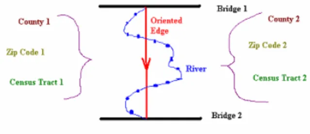
Figure 1: Illustration of the role of shape points. To illustrate the role of shape points, imagine a winding river that is crossed by two bridges a mile apart, and that the river is a county boundary and therefore of interest to the user (see Figure 1). The erratic path of the river requires many points to define it, but the regions on either side of it do not change from one point to the next, only when the next bridge is reached. In this case, the two bridge/river intersections would be the end points of an edge and the exact path of the river would be represented as shape points. As a result, only one set of polygons (one on either side of the river) is necessary to represent the boundary information of many small, shape defining edges of a boundary.
This kind of vector representation has significant advantages over other methods in terms of storage space. To illustrate this point, consider that many
boundaries will share the same border edges. These boundaries belong to not only neighboring regions of the same type, but also to different kinds of regions in the geographic hierarchy. As a result, storing the data contained in the TIGER/Line files in a basic location list data structure (LLS) such as ESRI Shapefiles, where every boundary stores its own latitude/longitude point, would introduce a significant amount of redundancy to an already restrictively large data set.
In contrast to its apparent storage efficiency, the TIGER vector data representation is very inefficient for boundary information retrieval and requires extensive processing. From a retrieval standpoint, an efficient representation would enable direct recovery of the entire boundary of a region as a list of consecutive points. The conversion between the memory efficient (concise) and retrieval efficient forms of the data is quite laborious in terms of both software development and computation time.
Another advantage of the TIGER/Line file representation is that each type of GIS information is self-contained in a subset of files. As a result users can process only the desired information by loading a selected subset of relevant files. For example, each primary region (county) is fully represented by a maximum of 17 files. Therefore, the landmark information is separate from the county boundary definition information, which is separate from the street address information, etc. Those files that are relevant to the boundary point extraction, and the attributes of those files that are of interest, are the following:
• Record Type 1: Edge ID (TLID), Lat/Long of End Points
• Record Type 2: TLID, Shape Points
• Record Type I: TLID, Polygon ID Left, Polygon ID Right
• Record Type S: Polygon ID, Zip Code, County, Census Tract, Block Group, etc.
• Record Type P: Polygon ID, Internal Point (Lat/Long).
We denote this subset of files as “Census boundary records”.
3.2
Theoretical Evaluations
This work extends our previous study about the tradeoffs between U.S. Census Bureau TIGER and ESRI Shapefile data representations that are documented in [7].
4
ESRI Shapefiles
A shapefile is a special data file format that stores non-topological geometry and attribute information for the spatial features in a data set. The geometry for a feature
is stored as a shape comprising a set of vector coordinates in a location list data structure (LLS). Shapefiles can support point, line, and area features. Area features are represented as closed loop polygons.
4.1
File Format Description
A shapefile must strictly conform to the ESRI specifications [4]. It consists of a main file, an index file, and a dBASE table. The main file is a direct access, variable-record-length file in which each record describes a shape with a list of its vertices. In the index file, each record contains the offset of the corresponding main file record from the beginning of the main file. The dBASE table contains feature attributes with one record per feature. The one-to-one relationship between geometry and attributes is based on record number. Attribute records in the dBASE file must be in the same order as records in the main file.
All file names adhere to the ESRI Shapefile 8.3 naming convention. The 8.3 naming convention restricts the name of a file to a maximum of 8 characters, followed by a 3 letter file extension. The main file, the index file, and the dBASE file have the same prefix. The suffix for the main file is ".shp". The suffix for the index file is ".shx". The suffix for the dBASE table is ".dbf".
Examples:
1. main file: counties.shp 2. index file: counties.shx 3.DBASE table: counties.dbf
The implementation of shapefile loading, writing and visualization routines was straightforward since the I2K ShapeObject data structure maps directly to the shapefile file organization.
4.2
Theoretical Evaluation
There are numerous reasons for using ESRI Shapefiles. ESRI Shapefiles do not have the processing overhead of a topological data structure such as a TIGER file. They have advantages over other data sources, such as faster drawing speed and edit ability. ESRI Shapefiles handle single features that overlap or are noncontiguous. They also typically require more disk space but are easier to read and write. However, the drawbacks of ESRI Shapefiles are in their storage inefficiency and poor scalability. We will quantify these tradeoffs in the experimental section.
5
Experimental Evaluations
In this section, our goals are (a) to experimentally evaluate the tradeoffs between storage and retrieval efficiency, and (b) to explain the tradeoffs by comparing fundamental format differences. In order to perform experimental tradeoff evaluations, we used two
datasets including (1) the SSURGO soil boundaries for Madison County, IL, stored in DLG-3 file format and (2) the U.S. Census Bureau boundaries of Illinois counties, zip codes, census block and census tracts stored in TIGER/Line file format. The preparation of these two data sets is outlined in Section 5.1. The results of all experiments are provided in Sections 5.2 and include comparisons of DLG & LLS, and DLG & TIGER & LLS. Sections 5.3, 5.4 and 5.5 explain the pair-wise format comparisons based on the experimental results.
5.1
Data Preparation
It is apparent that the experimental evaluations will depend on the size of test data. Ideally, one would like to show results as a function of input file size. However, the practical difficulty arises when one is looking for those test data sets that contain identical boundary information but are represented by LLS, TIGER and DLG files. We were not able to find such files.
We explored the possibility of finding software tools that would convert vector files from one file format to another so that we could create multiple test files with identical boundary information stored in LLS, TIGER and DLG formats. We have concluded that while LLS formats (ESRI Shapefiles) are supported by most GIS software packages, there is a very limited support for DLG and TIGER file formats. This corresponds to our assessment of the implementation complexity to support loading of TIGER, DLG and LLS formats in this order from the most time consuming to the least time consuming. The implementation effort usually doubles when both loading and writing routines have to be supported.
Based on our findings about conversion tools and the availability of GIS software packages at our institution, we created data sets by (1) implementing TIGER to LLS, and DLG to LLS conversions, and (2) using ArcToolBox for LLS to DLG conversion. We created several test data sets that are described next.
In the first experimental tradeoff evaluation, we used a file pair consisting of the original DLG file (SSURGO soil boundaries) and the LLS file converted using I2K. This file pair is denoted as the test data set #1.
In the second experimental tradeoff evaluation, we prepared a triplet of files consisting of (a) the original TIGER files for the state of Illinois, (b) the LLS files obtained by extracting the U.S. Census Bureau boundaries of counties, zip codes, census block and census tracts from the TIGER files and converting them by using our software implementation, and (c) the DLG file converted from the already obtained LLS file using ArcToolBox. This triplet of files provides a test data set for fair performance evaluations in terms of “Total Load Time” and Load RAM Required” parameters. However, this test data set cannot be used for
performance evaluations in terms of “Hard Disk” because the TIGER files include all boundary types (including voting districts, and so on), of which four were extracted to LLS and DLG file formats. This file triplet is denoted as the test data set #2.
We expanded the second experimental tradeoff evaluations in Section 5.2 by partitioning the test data set #2. We used sub-sets of the original TIGER files for the state of Illinois in order to vary the number of nodes. In order to explore load time dependency on the number of nodes (boundary points), we selected 1, 2, 3, 4, 10, 15, or 24 counties from the original TIGER files, and formed several triplets of test data sets (TIGER, LLS and DLG). We always chose a subset of counties forming geographically contiguous regions so that neighboring counties would have some overlap of boundary points. This set of file triplets is denoted as the test data set #3.
5.2
TIGER, LLS, and DLG Tradeoff
Evaluations
The experimental results of our tradeoff evaluations between storage and retrieval efficiency are presented in Tables 1 and 2. As described in the previous section, the test data sets #1 and #2 {(DLG, LLS) and (TIGER, LLS, DLG)} were formed from the original DLG and TIGER files by converting them into other file formats
using Arc ToolBox and our software. Each file format was then read in separately, and the storage and loading measurements were recorded in Tables 1 and 2.
Before explaining the experimental results by comparing pairs of file formats presented in Sections 2, 3 and 4, we posed the following two questions. First, is there any dependency of storage on the boundary content? In other words, if we had a file with watershed and zip code boundaries, would the results be different from evaluating Census tracts and blocks, and how? Second, can we predict the total load time as a function of the number of polygons/nodes without exhaustive experimentation? Or in other words, what would be the dependency between boundary information retrieval and the number of retrieved nodes?
Storage Dependency on Boundary Content: The answer to the first question is related to the amount of boundary overlap. Ideally, one would experiment with sets of boundaries that span cases from a zero overlap (e.g., non-adjacent county boundaries) to an overlapping hierarchy of polygons (census blocks, block groups and tracts). Our data sets represent the cases of partial overlap (SSURGO) and large overlap (TIGER) of boundaries. Thus, the experimental results will vary as a function of boundary content in the following way: the more overlapping boundaries, the smaller hard disk requirements for TIGER format in Table 2: Test data#2: U.S. Census Bureau 2000 TIGER/Line files for the state of Illinois (102 counties). Loading is constrained to block groups, zcta, census tract, and counties ((Total Load Time and Load RAM Required parameters). Hard Disk and Number of Nodes measurements for LLS and DLG formats contain only block groups, zcta, census tract, and county boundaries, whereas the same measurements for TIGER format include all types of boundary information for the state of Illinois.
Total Load Time
(s) Hard Disk (MB) Unzip Load RAM Required (MB) Zip Unzip Number of Nodes TIGER 1300.2 200 112 940 2,176,719 LLS 12.7 37 27 47 641,955 DLG-3 12.9 52 8 24 457,850 Table 1: Test data#1: SSURGO Soil Database, Madison County, IL. Loading time includes all SSURGO soil
boundaries. Hard disk measurements pertain to all boundaries in the original SSURGO files. Total Load Time
(s) Hard Disk (MB) Zip Unzip Load RAM Required (MB) Zip Unzip Number of Nodes LLS (Shapefile) 41.36 290 65 90 2,787,490 DLG 105.72 103.72 380 23 79 2,787,790
comparison with DLG and LLS (in this order), and the smaller load RAM requirements for LLS format in comparison with DLG and TIGER.
Our conclusion is supported by comparing the number of loaded nodes versus the number of unique nodes using the test data sets #1 and #3, and by inspecting the LLS files. By evaluating the ratio s of these two numbers (loaded nodes versus unique nodes) using the test data #2 (partial boundary overlap), we obtain s equal to 2.02 (5630800/2787490). The same evaluation of the ratio s using the data set #3 (large boundary overlap) led to an average ratio value equal to 2.6416. The measurements using the test data set #3 (ZCTA, Block Group (BG), Census Tract (CT), and County boundaries for 1, 2, 3, 4, 10, 15, and 24 Illinois counties) are shown in Figure 2.
We took additional measurements to compute the ratio s for (a) watershed and county boundaries (s = 84,601/47,636=1.776), and (b) watershed and ZCTAs boundaries (s=344,533/201,767=1.708). We observed that approximately 70% of the points in both (a) and (b) are shared between multiple boundaries. Thus, the inefficiency of LLS format due to the duplicate points of neighboring boundaries would not decrease below s=1.7 for the test data.
LLS File Format y = 2.6416x + 2281.2 R2 = 1 0 50000 100000 150000 200000 250000 300000 350000 400000 0 20000 40000 60000 80000 100000 120000 140000 Number of Unique Nodes
N um be r of Loa d ed N ode s
Figure 2: Storage efficiency measurements of LLS files using the test data set #3 (Hierarchical boundary content). The points correspond to evaluations for data sets with boundaries for 1, 2, 3, 4, 10, 15, and 24 Illinois counties.
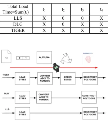
Boundary Information Retrieval Dependency on Number of Nodes: In order to answer the second question about the relationship between a load time and a number of nodes, we divided the Total Load Time into four components: t1, t2, t3 and t4 (see Equation below and Figure 3). The first component t1 corresponds to the time to construct polygons from an ordered list of edges. The second component t2 is for the time to create an ordered list of edges from an unordered set of edges. The third component t3 represents the time to convert ASCII characters to numeric type values. The last component t4 is the time
to load any sequence of bytes (ASCII characters or binary values) from a file. We introduce these time components based on our understanding of the three vector file formats.
1 2 3 4
Total Load Time t
= + + +
t
t
t
(1)The zero and non-zero time components are summarized for each file format in Table 3. The total load time as a function of the number of nodes can be predicted by knowing that the time components t1, t2, t3 and t4 are linear with the increasing number of nodes. The quadratic dependency of the time component t2 (creation of ordered list of edges) as a function of the increasing number of nodes is avoided by the fact that the unordered edges are grouped by counties rather than by states. Based on our empirical observations,
1 2 3
t
< <
t
t
for a fixed number of nodes, which leads tosuperior total load time for LLS format in comparison with DLG and TIGER formats (in this order). Our theoretical predicted Total Load Time as a function of the number of nodes is shown in Figure 3 and is independent of test data sets (addressed as the question number 1 above).
Table 3: Total Load Time decomposition. Total Load
Time=Sum(ti) t1 t2 t3 t4
LLS X 0 0 X
DLG X 0 X X
TIGER X X X X
Figure 3: Total Load Time decomposition for TIGER, DLG and LLS file formats.
Figure 4 : Theoretically predicted Total Load Time as a function of the number of nodes.
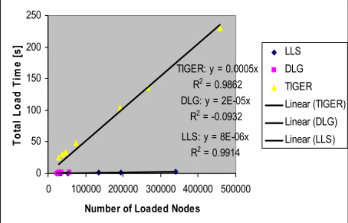
We have obtained experimental measurements that support our theoretically predicted Total Load Time dependency on the number of nodes using the test data set #3. Figure 5 shows our measurements and linear trends, where the points correspond to data sets with boundaries for 1, 2, 3, 4, 10, 15, and 24 Illinois counties. These supporting measurements for “Total Load Time” and “Load RAM Required” were calculated by averaging three runs to load the ZCTA, Block Group (BG), Census Tract (CT), and County boundaries for each data set. The total number of nodes and the number of unique nodes were measured (a) by counting nodes inside of our software developed for loading LLS and DLG files, and (b) by summing end points and shape points for TIGER files according to the accompanying TIGER documentation. While TIGER files do not contain any duplicate points, LLS duplicate points were found using a hash table in our software. TIGER: y = 0.0005x R2 = 0.9862 DLG: y = 2E-05x R2 = -0.0932 LLS: y = 8E-06x R2 = 0.9914 0 50 100 150 200 250 0 100000 200000 300000 400000 500000
Number of Loaded Nodes
Tot al Loa d Ti m e [ s] LLS DLG TIGER Linear (TIGER) Linear (DLG) Linear (LLS)
Figure 5 : Total Load Time vs. Number of Nodes for 1, 2, 3, 4, 10, 15, and 24 counties with a best-fit line.
According to Figure 5 and based on our test data set #3, the total loading time for TIGER files is approximately 40 times slower than for LLS files, and
the total loading time for DLG files is about 2.5 times slower than for LLS files. We collected measurements for only 1, 2, 3 and 4 county aggregations in the case of DLG format because the data preparation is very time consuming.
5.3
DLG and LLS Comparisons
The DLG optional and LLS (or ESRI Shapefile) formats specify boundaries over an area. Both formats have geographic information that allows the boundaries to be geo-referenced with other data sources. The formats differ in how the data is structured and stored.
The first primary difference between DLG and LLS is that DLG is stored in an ASCII format, while LLS is stored in a binary format. DLG files are comprised of ASCII characters organized into fixed-length logical records of 80 characters. When loading a DLG file, all data contained within must be converted to native data types. For example, a coordinate is stored as the ASCII characters “4598829.0” in the file. This must be read in and converted to its numeric value. ESRI Shapefile, on the other hand, stores the data as a series of bytes that can be quickly converted to a data type. For the previous example, the value “4598829.0” would be stored as 8 bytes that can be directly converted into a numeric value However, it may be necessary to reverse the order of the bytes to account for the byte order (little or big endian). The reading (and possible reversing) of bytes for a shapefile is far simpler than the ASCII-to-native transformation needed for DLG.
This primary difference in representation (ASCII vs. binary) greatly affects the loading times of the two approaches. Each entry in a DLG soil database must be read individually, and then converted to a numeric value. This is the most time-consuming operation when loading the data, typically over 25% of the loading time of a DLG file. Loading ESRI Shapefile, however, is much quicker. It is simply reading a series of bytes from a file, with little conversion needed. This quickness comes at the price of a larger file size for the ESRI Shapefile. In an examination of one county, the DLG data needs approximately 79 MB of disk space uncompressed, 23 MB compressed. The ESRI Shapefile, on the other hand, needs 90 MB of disk space when uncompressed, and 65 MB when compressed. These results are summarized in Table 1 and Table 2. The difference in compressed sizes between the two encodings is attributable to their physical representations. DLG data contains fixed-length records with white space between elements to maintain the fixed length. This white space is insignificant and can be easily compressed. On the other hand, all binary data in an ESRI Shapefile are significant and cannot be easily compressed.
The second difference between DLG and LLS is the way how the data in a file are structured. DLG format uses nodes, lines, and areas to define its polygons. In
each of the SSURGO DLG datasets examined so far, nodes have not been used to define lines or areas. The lines are a series of coordinate values, and the areas have a list of the lines that make up the area. On the other hand, LLS format lists the bounding box and the points for each boundary contained within it. DLG format makes more efficient usage of space; areas that share lines will both reference the same line, while in a shapefile, each coordinate, including coordinates shared between different boundaries, is explicitly listed. In addition, this difference makes it necessary to first read all the lines in a DLG file before reading in the areas, because the areas are made up of a list of the lines. The lines have to be kept in a lookup table, and areas cannot be fully processed until all lines have been read.
The consequence of the second difference between DLG and LLS is that different data structures have to be used when loading these files. Our goal is to have one ShapeObject that contains all the polygons in a soil database. DLG format gives no hint as to how many points will be needed to store all the polygons in the DLG file. Furthermore, it does not give the bounding box for each polygon. In contrast, ESRI Shapefile stores these values so that it is possible (a) to pre-compute the space requirements needed and (b) to allocate arrays to hold the data when loading a Shapefile. With DLG, however, it would only be possible to pre-compute the sizes by reading in all data files twice. One time to determine the sizes, and one time to actually read in the data. In addition, the bounding box for each polygon is not stored in DLG, and must be found while reading in the coordinates of each area. This requires comparisons for each coordinate to find the bounding box. In our implementation, expandable arrays (or vectors) were used so that the files only had to be read in once. Then, once fully read, the data are copied into an array in the ShapeObject, of the exact size needed. The problem with this approach is that when the copy is made, two arrays must exist in memory. The first will be the array that contains the vector data. The second will be the new ShapeObject array to copy the contents of the vector into. This causes the memory requirements of DLG-3 files to balloon to twice the total necessary size in the worst case, when copying all the individual points of all the polygons into one ShapeObject.
The third difference between DLG and LLS is related to georeferencing information. SSURGO DLG files are stored as quarter-quadrangles. Each quadrangle represents 7.5 minutes of a degree of longitude and latitude. It is necessary to load 64 individual files to represent a one degree block. ESRI Shapefile does not need to be represented this way. However, Shapefiles could be stored in this way, if desired. All coordinates in SSURGO DLG files are stored in UTM format. This causes problems when geo-referencing the boundaries in I2K because the state of Illinois is located in both UTM zone 15 and UTM
zone 16. The solution was to immediately translate the UTM coordinates to latitude and longitude. Over 29% of the time to load a SSURGO DLG file was spent in the conversion from UTM coordinates to latitude and longitude. Each DLG file contains the UTM zone in the header information. ESRI Shapefile normally contains latitude and longitudinal geo-referencing information. No conversion was required when loading the shapefile in I2K. A potential drawback of the ESRI Shapefile format is that there is not a standard way to define the projection used in for the coordinates. DLG has a value in the header to signify if UTM or Albers projection is used. Also, some of the projection parameters are stored in the header of a DLG. Shapefiles, on the other hand, do not store projection information. This information could be stored with the meta data for a shapefile, but it is not required. This makes it difficult to distribute shapefiles with geo-referencing information other than standard latitude and longitude.
5.4
DLG and TIGER Comparisons
DLG and TIGER offer similar methods to encode vector data. TIGER’s use of an edge with shape points corresponds directly to DLG’s use of lines and coordinates. Likewise, a TIGER polygon is comprised of a series of edges, and a DLG area is made up of a series of lines. This provides a compact, human-readable representation of the vector data.
The two formats differ in the type of data that are encoded. DLG format typically encodes one layer of data in a file, such as the soil types used by SSURGO. Other layers, such as water boundaries, are encoded in separate files. This scheme introduces some redundancy between the layers. Layers are unrelated to one another, and any shared boundaries will be specified in each layer. For example, a soil layer encoded as a DLG may have boundaries defined along a river. A layer containing bodies of water may share the same boundaries, but the points will be specified again because the soil layer is unrelated to the body of water layer in DLG. TIGER format, on the other hand, groups all edges together, regardless of layer. The different metadata files are used to determine which edges to use. This format allows for less redundancy.
Polygons are retrieved very differently by the DLG and TIGER loaders. DLG format specifies the exact boundaries for each polygon. A list of lines defines the exact border of a polygon, and the lines are in the proper sequence. Since the lines appear in the proper sequence, the polygon can be quickly constructed after all line retrieval. In contrary to DLG format, the boundaries stored in TIGER format must be found programmatically. Each edge is labeled with the polygons that appear on the left and right of the edge. To construct a polygon A, you must first find all edges that border the polygon A. The edges only define the
end points of each edge, and not the order in which the edges should be connected. So the boundary of polygon A must be constructed programmatically by comparing the end points of each edge. Thus, the TIGER polygon construction is far more complex and time-consuming than the DLG polygon construction.
5.5
TIGER and LLS Comparisons
One can derive TIGER and LLS comparisons from the description provided in Sections 2, 3 and 4 that compare DLG and LLS, and TIGER and DLG formats. Since the experimental tradeoff evaluations of TIGER and LLS are summarized in Table 2, we devoted this section to the implementation of TIGER to LLS conversion.
The underlying principle of the conversion process from TIGER/Line files to ESRI Shapefiles could be compared to sorting points according to the order of boundary edges. This is illustrated in Figure 4. In reality, the conversion process begins by loading the raw TIGER/Line files into 2-D table-like data structures by making use of manually developed meta data files. Since the TIGER/Line files are fixed-width encoded flat files, meta data is necessary to define the indices of the first and last characters for each attribute in the lines of the flat file. This information, the attributes’ names, and their type (integer, floating point number, string, etc) come from meta data files provided by the Census Bureau. The final piece of information contained in the meta data file is a “Remove Column” field, which dictates whether or not the attribute will be dropped from the table as it is read in. Attributes that are not used during the processing are removed early on for the sake of memory efficiency. The meta information for each Record Type is stored in a comma-separated-value (csv) file, which can easily be parsed into a table object, then accessed in that form by the routine that parses the main data file.
Once the TIGER/Line data are in the form of tables, they are streamed through a complex system of procedures, including conversion to several intermediate data structures, before being inserted into Hierarchical Boundary Objects (HBoundary) [7]. Each HBoundary represents one type of region (county, census track, etc) for a single state. It can also be viewed as one master list of boundary points that all boundaries reference by pointers. The RAM memory savings of HBoundary versus ShapeObject for each point that is shared by two counties, two census tracts, and two block group boundaries is 30 bytes. For the state of Illinois, this optimization translated into a 38% reduction in memory usage (16.45 MB versus 26.64 MB).
Figure 6: The TIGER/Line to ESRI Shapefiles
conversion of boundary representation can be viewed as a transformation from an unordered set of points to a clock-wise ordered set of points.
Finally, the HBoundary object is converted into LLS format by constructing all polygons. The resulting LLS format file was tested by loading it into the commercial ArcExplorer software package [3]. For our experimental tradeoff evaluations, we extracted only a selected subset of Census boundary records from the Census 2000 TIGER/Line files. Thus, it is hard to evaluate loading RAM requirements for TIGER and other two formats since the HBoundary object contains all hierarchical boundaries and their associated information, while the converted LLS file contains only four types of boundaries (counties, ZCTAs, blocks and tracts) and extracted information about region names, neighboring regions to each boundary, and an internal point of each region.
6
Summary
In this paper we have investigated the storage and retrieval efficiency tradeoffs between the ESRI Shapefile (LLS), DLG, and TIGER formats. LLS files will provide the fastest method for boundary retrieval (40 times faster than TIGER and 2.5 times faster than DLG). All boundaries are stored in a binary format for quick retrieval. This speed comes at the price of file size. Each boundary in a LLS file contains all the points that make up the boundary. This introduces storage redundancy (between 70% and 180% redundancy in our experiments) since boundaries can be shared between different polygons. Digital Line Graphs reduce the amount of redundant data. This reduction is tempered by the need for more retrieval processing per boundary. The TIGER format further reduces the amount of data. TIGER format is the most compact representation that comes at the cost of the highest boundary retrieval requirements. Detailed information about these results can be found in Reference [12].
trade-offs between storage and boundary retrieval requirements for the three vector files. The measurements about “Total Load Time”, “Load RAM Required” and “Hard Disk” as a function of “Number of Loaded/Unique Nodes” were used as our metric to demonstrate the trade-offs. Our measurements support the existing knowledge about the choice of a file format depending on the data content that is mapped to boundary overlaps. However, there are other metrics that might affect institutional decisions as well, and were not included in this study. We could enumerate a few metrics, such as (1) a cost of storage media and RAM, (2) a cost of software development to support complex file formats, (3) a preservation of storage media, (4) an availability of software tools for ingesting and processing certain file formats, or (5) an open source implementation of software tools that would allow tracking discrepancies in file format interpretation (loading) and replication (writing). While we did not quantify the additional possible metrics, we have made the following observations. First, numerous software tools support the ESRI Shapefile format whereas not many tools work with Digital Line Graphs or TIGER files. Second, the amount of time we have spent implementing the LLS, DLG and TIGER file format loaders was increasing in the order of the listed file formats. We hypothesize that the increase is almost linear but it becomes quadratic as the file format is too complex to track and eliminate software bugs. Finally, the cost of storage and RAM has been rapidly decreasing over the last decade. We could not foresee the future technological advancements of storage media that would favor one file format over another.
7
Future Directions
One would like to incorporate the effects of computer clusters and mass storage systems on the storage versus boundary retrieval efficiency tradeoff evaluations for LLS, TIGER and DLG data structures. Our tradeoff study thus far has been in an isolated workstation environment. The results of our tradeoff study could differ when a very large cluster or mass storage system is used. We have identified several directions that further research could take.
First, investigate the effect of computer clusters on boundary retrieval efficiency assuming distributed or centralized locations of a large number of boundary files. The benefit of using a computer cluster would come from parallelization of loading and boundary reconstruction tasks.
Second, empirical results and theoretical analyses from our research thus far have shown file size (computer storage size) to be related to the amount of overlap between boundaries. The usage of a mass storage system will add to the time needed to load bytes from a file.
Another component of mass storage systems and
computer cluster environments is the Input/Output (I/O) bandwidth and I/O schemes. While the relationship between I/O bandwidth and boundary retrieval efficiency is straightforward (linear dependency), there are a few questions to ask about I/O schemes. For instance, can more efficient I/O schemes be used to improve boundary retrieval? Would message passing interface input/output (MPI-IO) have any effect? What would be the bottlenecks?
Finally, our ultimate goal is to understand multiple effects of electronic vector files on the archival process. We could mention just a few effects, such as vector file format, data organization and representation, algorithmic parallelization, scalability of vector file loading in terms file size and centralized or distributed file locations, software re-usability, computer platform dependency, computer cluster environments, I/O bandwidth and I/O schemes, and mass storage systems.
Acknowledgements
This research was supported by a National Archive and Records Administration (NARA) supplement to NSF PACI cooperative agreement CA #SCI-9619019. The views and conclusions contained in this document are those of the authors and should not be interpreted as representing the official policies, either expressed or implied, of the National Science Foundation, the National Archives and Records Administration, or the U.S. government.
References
[1] Campbell, James B. Introduction to Remote Sensing, Second Edition. The Guilford Press, New York. 1996.
[2] Miller, Catherine L. TIGER/Line Files Technical Documentation. UA 2000. U.S. Department of Commerce, Geography Division, U.S. Census Bureau.
http://www.census.gov/geo/www/TIGER/TIGERu a/ua2ktgr.pdf
[3] ArcExplorer, ESRI web site: http://www.esri.com
[4] ESRI Shape file, File Format Specification,
http://www.esri.com/library/whitepapers/pdfs/shap efile.pdf
[5] Bajcsy P. et. al., “Image To Knowledge”, documentation at web site:
http://alg.ncsa.uiuc.edu/tools/docs/i2k/manual/inde x.html.
[6] Alumbaugh T.J. and Bajcsy P.,”Georeferencing Maps with Contours in I2K”, ALG NCSA technical report, alg02-001, October 11 2002. [7] Groves P., S. Saha and P. Bajcsy, “Boundary
Information Storage, Retrieval, Georeferencing and Visualization,” Technical Report NCSA-ALG-03-0001, February 2003.
web site:
http://alg.ncsa.uiuc.edu/tools/docs/d2k/manual/inde x.html
[9] “Digital Line Graph References” prepared by the Office of Information Technology,
http://www.oit.ohio.gov/SDD/ESS/Gis/DigitalLine Graphs.aspx#Documentation
[10] Digital Line Graphs from 1:24,000-Scale Maps Data Users Guide 1,
http://www.geodata.gis.state.oh.us/dlg/usrguide/usr guide.htm
[11] “US GeoData, Digital Line Graphs” prepared by the U.S. Department of the Interior and the U.S. Geological Survey,
http://www.usgsquads.com/downloads/factsheets/u sgs_dlg.pdf
[12] Clutter D. and P.Bajcsy. “Storage and Retrieval Efficiency Evaluations of Boundary Data Representations for LLS, TIGER and DLG Data Structures,” Technical Report NCSA-ALG-04-0007, October 2004.