Color Reduction Using Local Features and a Kohonen
Self-Organized Feature Map Neural Network
Nikos Papamarkos
Electric Circuits Analysis Laboratory, Department of Electrical and Computer Engineering,
Democritus University of Thrace, 67100 Xanthi, Greece. E-mail: [email protected]
ABSTRACT: This paper proposes a new method for reducing the number of colors in an image. The proposed approach uses both the image color components and local image characteristics to feed a Kohonen self-organized feature map (SOFM) neural network. After training, the neurons of the output competition layer define the proper color classes. The final image has the dominant image colors and its texture approaches the image local characteristics used. To speed up the entire algorithm and reduce memory requirements, a fractal scan-ning subsampling technique can be used. The method is applicable to all types of color images and can be easily extended to accommodate any type of spatial characteristics. Several experimental and compar-ative results are presented.© 1999 John Wiley & Sons, Inc. Int J Imaging Syst Technol, 10, 404 – 409, 1999
I. INTRODUCTION
Color is one of the most important properties for object discrimina-tion. It is an object component that adds a new dimension to machine vision. Limitations of possible applications of color machine vision have been associated with the high cost and low processing capa-bility of added information. On the other hand, color is a very significant characteristic that cannot be ignored in many machine vision applications. Its use in image segmentation and recognition systems can hardly be overestimated. Various color-based image segmentation techniques have been proposed. Ohta et al. (1980) applied the Karnhunen Loeve transform to color images to derive color features with large discrimination power. Connah and Fish-bourne (1981) reported an algorithm based on the histogram analysis of color gray-level distribution. Huntsberger and Delxazi (1985) reported a color edge detector that uses fuzzy set theory. Barth et al. (1986) presented a microcomputer color-based vision system to inspect integrated circuits. Tominaga (1990) described a color clas-sification method based on the Lab uniform color space. Represen-tative colors are classified according to a color distance criterion. Jordan and Bovik (1988) used chromatic information to solve stereo vision problems. Valchos and Constantinides (1993) proposed an algorithm, based on color and graph theory, most suitable for ap-plications such as broadcasting and pictorial information retrieval. Schettini (1994) presented a color image segmentation technique based on recursive one-dimensional (1-D) histogram analysis. The resulting regions are merged based on a criterion taking into account color similarity and spatial proximity.
Reduction of the image colors is an important factor for the segmentation, compression, presentation, and transmission of
im-ages. In most cases, it is easier to process and understand an image with a limited number of colors. However, the main reason for using color reduction is to cut down the image storage requirements. In gray-level images, the most often used reduction techniques are the multithresholding approaches. These techniques can be classified into three categories. Methods based on edge matching and classi-fication belong in the first category (Sahoo et al., 1988; Wang and Haralick, 1984; Hertz and Schafer, 1988). The histogram-based multithreshold techniques belong in the second category (Reddi et al., 1984; Kapur et al., 1985; Papamarkos and Gatos, 1994; Otsu, 1979). These techniques are based on different criteria such as the minimum entropy, the interclass variance between dark and bright regions, and changes of zero crossing or curve fitting. Finally, the third category includes all the other techniques, which usually are characterized as hybrid. It should be noted that none of the mul-tithresholding techniques take into account the local texture charac-teristics of an image.
The aforementioned techniques cannot be easily extended to accommodate color images. Extension of these techniques to mul-tispectral images and in particular to color images is not a trivial task. The main reasons are the increasing complexity and the struc-ture of the natural color scenes. The most often used methods for color reduction are based on nearest color merging or color error diffusion. In the nearest color methods, each pixel in the image changes its color to the color in a palette that is the closest match to some typical neighboring pixels. A color palette is a fixed color table that has a limited number of colors. There are two approaches to form the colors in the color table. We can use a fixed palette of colors that someone has already produced or we can analyze the image and derive the “best” colors (known as an adaptive palette). The adaptive technique consists of first analyzing the image and selecting the best colors to represent it and second, mapping the original color dots to the closest of the new colors. However, the choice of “the best” colors is not a trivial task. Most adaptive algorithms determine how many dots of each color are in an image and select colors that are close to the most frequently used colors. The error diffusion techniques are dithering approaches. The “error” refers to the cumulative difference between the actual values of pixels in the image and their “true” values, if they were all set to their correct colors. These techniques are suitable for elimination of less frequently appearing colors in an image but are ineffective for image analysis and segmentation.
This paper proposes a new color reduction method that exploits the colors of the pixels as well as the local spatial image character-istics. The color reduction process does not use a color palette. The final colors are automatically selected by a neural network-based color clustering approach. The color of each pixel is related to the colors and the texture of neighboring pixels. The new technique can be considered as a feature clustering approach. Specifically, the RGB components of each pixel are considered to be the first three features. The entire feature set is completed by additional features that are extracted from neighboring pixels. These features can be associated with spatial image characteristics, such as entropy, con-trast, and mean values. The feature set feeds a Kohonen self-organized feature map (SOFM), which is an unsupervised neural network (Kohonen, 1997; Haykin, 1994; Strouthopoulos and Pa-pamarkos, 1998). The SOFM is competitively trained, according to Kohonen’s learning algorithm. After training, the output neurons of the SOFM define the proper feature classes. Next, each pixel is classified into one of these classes and obtains the color of the class. Thus, the original image is converted into a new one with a limited number of colors and spatial characteristics close to those defined by the features used. Compared with other neural networks, and espe-cially with supervising learning, competitive learning is highly suited to discovering a feature set and creating new classes auto-matically (Haykin, 1994). The SOFM has the ability to discover significant features in the input data without a teacher. In addition, it is preferable to use a self-organizing process instead of a super-vising process to solve a particular problem.
Due to the use of local image characteristics, the proposed technique is especially suitable for segmentation and compression and representation of color images. In order to reduce both the storage requirement and computation time, the training set can be a representative sample of the image pixels. In our approach, the subsampling is performed via a fractal scanning technique based on the Hilbert’s space filling curve (Sagan, 1994).
The proposed method was tested using a variety of images. In addition, this paper presents characteristic examples with various image local characteristics. The experimental and comparative re-sults confirm the effectiveness of the proposed method.
II. DESCRIPTION OF THE METHOD
A color image can be considered as a set of n3m pixels, where
each pixel is a point in the RGB color space. RGB space is a 3-D vector space and each pixel (i, j) is defined by an ordered triple of red, green, and blue coordinates, (r(i, j), g(i, j), (b(i, j)). Therefore, a general image function can be defined by the relation:
I~i, j, k!5
H
r~i, j!, if k51,
g~i, j!, if k52,
b~i, j!, if k53
(1)
Each primary color component (red, green, or blue) represents an intensity that varies linearly from zero to a maximum value, Cmax. Color allocation is defined over a domain consisting of a cube in RGB space, with opposite vertices at (0, 0, 0) and (Cr_max,
Cg_max, Cb_max). Consider the case of Cr_max 5 Cg_max 5 Cb_max5255.
Let also N (i, j) denote the neighboring region of pixel (i, j). In most cases, it can be assumed that pixel (i, j) belongs to N (i, j). In this approach, N (i, j) is the 333 mask that has as its center the pixel (i, j). In most cases, the color of each pixel is associated with the
colors of the neighboring pixels and the local texture of the image. For these reasons, the color of pixel (i, j) can be associated with local image characteristics extracted from the neighboring region N (i, j). Using the color values of N (i, j), fk, k51,2, . . . , K local charac-teristics can be defined, and these are considered as image spatial features. Through this, each pixel (i, j) can be related with its (r(i, j),
g(i, j), (b(i, j)) components and with the K additional features fk. No restrictions are implied for the type of features. However, the fea-tures must represent simple spatial characteristics, such as contrast, median RGB values, and entropy of the neighboring masks. Such features can be associated with linear or nonlinear operators and can be easily extracted by the application of local masks.
According to the above analysis, the color reduction problem is how to best transform the original color image to a new one, with only J colors and with, approximately, the same local characteristics. An effective approach is to view it as a clustering problem and solve it by using a suitable SOFM neural network. It is well known that the main goal of an SOFM neural network is the representation of a large set of input vectors with a smaller set of “prototype” vectors, so that a “good” approximation of the original input space can be obtained. In other words, an SOFM neural network decreases the input feature space into a proper smaller one. The resultant feature space is a representative of the original feature space and, therefore, it satisfies the main statistical characteristics of the input space.
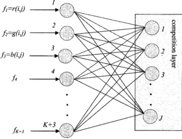
A. The SOFM Neural Network. The structure of the Kohonen SOFM neural network used is depicted in Figure 1. It has K1 3 input and J output neurons arranged in a 1-D grid. The first three input neurons are fed with the values of the RGB components of pixel (i, j). The rest of the K neurons correspond to the local features
fk, k51,2, . . . , K and are fed with their values. Each neuron in the competition layer represents one class, which is associated not only with the RGB values, but also with the spatial features used. Ad-justing the number of the output neurons, the number of colors in the final image can be defined. The output J neurons are related to input neurons via the wi,j, i51, . . . , K13 and j51, . . . , J coefficients. The SOFM is competitively trained according to the following weight update function
Dwji5
H
a~yi2wji!, if uc2ju#d, 0, otherwise
i51, . . . , K13 and j51, . . . , J (2) where yj are the input values, a the learning parameter, d the neighboring parameter (a typical initial value is less than 0.25), and
c the winner neuron. The values of parameters a and d are reduced
to zero during the learning process. This learning algorithm has been referred to as Kohonen’s learning.
After training, the optimal RGB values obtained by the neural network are equal to
r~j!5w1,j, j51, . . . , J g~j!5w2,j, j51, . . . , J
b~j!5w3,j, j51, . . . , J
J
(3) Next, the original image is rescanned. Using the neural network, the new image is constructed with only J colors in such a way that approximates the spatial characteristics of the original image accord-ing to the spatial features used. However, if the spatial characteris-tics are not used, the neural network can be fed and trained using only the RGB colors. Obviously, this procedure results in a reduced set of RGB colors that are optimally (according to Kohonen’s learning rule) close to the color distribution of the original image.B. Color Conversion. As an optional postprocessing stage, the RGB colors obtained by using spatial features can be converted to the RGB colors derived when only the RGB components are used (Papamarkos et al., in press). Let I1and I2be the images obtained by using and not using spatial features, respectively. The color conversion can be easily implemented by checking the colors of the pixels in I1and I2 that have the same coordinates. Specifically, let
Cm
1 5
(rm, gm, bm), m51, . . ., J: the set of RGB colors in I1. Cm
2
5(rm, gm, bm), m51, . . ., J: the set of RGB colors in I2. Sm
2
, m51, . . ., J: the set of pixels I2that have the same color Cm
2 . Sm
1
, m 5 1, . . ., J: the set of pixels I1 that have the same coordinates with the pixels of the set Sm
2 in I2.
Pnm, (n,m)51, . . ., J: the percentage of pixels I1that belong to the set Sm
1
and have color Cn
1 .
Starting from the pixels having the maximum percentage, convert its color Cn
1
to the corresponding color Cm
2
. This optional stage provides an aesthetically better image, especially when there is a small number of final colors (small value of J).
C. Image Subsampling. The proposed technique can be applied to the color images without any subsampling. However, in the case of large color images, and in order to achieve reduction in compu-tation time and memory size requirements, it is preferable to have a subsampling version of the original image. The subsampling process should not alter the original image colors, but simply produce a smaller version of the image without significant changes in the image texture characteristics. For the subsampling image to be a better representation (to capture better the image texture) of the original, a fractal scanning process based on the well-known Hil-bert’s space filling curve was used. To generate the Hilbert curve,
Figure 2. Generation of the Hilbert curve.
Figure 3. Image subsampling using fractal scanning.
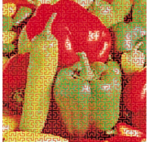
Figure 4 (a) The original image. (b) The transformed image with six colors using spatial features. (c) The transformed image without using spatial features. (d) The final image after color conversion.
start with the basic staple-like shape as depicted in Figure 2a. The rest of the Hilbert curve is created sequentially, using the same algorithm. Starting with the basic Hilbert curve in each step, in-crease the grid size by a factor of two. Then, place four copies of the previous curve on the grid. The lower two copies are placed directly as they are. The upper left quarter is rotated by 90° anticlockwise and the upper right quarter by 90° lockwise. Finally, connect the four pieces with short straight segments to obtain the next step curve (Fig. 2b,c). A complete description of the Hilbert’s curve is provided by Sagan (1994). If k is the order of the Hilbert’s curve, then the ratio of the subsampled image pixels over the total number of pixels is
4k
number of image pixels (4)
As an example, Figure 3 depicts a fractal image subsampling of a 2003200 pixel image with k57.
D. The Steps of the Method. According to the above analysis, the steps of the proposed color reduction technique are:
Step 1. Define the number J of the final colors and the number and type of the spatial features.
Step 2. Construct the SOFM neural network. Step 3. Decide if subsampling will be used. Step 4. Train the SOFM neural network.
Step 5. Using the neural network, transform the original image to a new one with the reduced number of colors obtained in Step 4.
Step 6. If it is required, obtain the optimal colors by repeating Step 4, without using the spatial features. Next, convert the colors obtained in Step 4 to the new color set.
III. EXPERIMENTAL RESULTS
The entire method has been implemented using MATLAB, version 5.1. The SOFM neural network is implemented using the neural network package of MATLAB and is also tested by the developer version 3.02 of NeuralSolution (NeuroDimension, Inc.; www. nd.com).
Experiment 1. Consider the original 256-color image shown in Figure 4a. The size of this image is 2003200 pixels with 96 dpi resolution. In this example and for every RGB component, the absolute difference between the pixel color and the mean color of the eight neighboring pixels was used as the spatial features. These features correspond to the Laplacian magnitude (Sonka et al., 1999) and can be considered as contrast features. Specifically, the three spatial features f4, f5, f6are calculated using the relation:
fk5
U
I~i, j, k23!2 1 8O
a521 1O
b521 1 I~i1a, j1b, k23!U
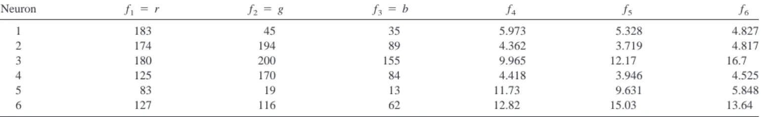
, ~a,b!Þ~0,0! k54, 5, 6 (5) The SOFM neural network is trained with only six neurons in the competition layer. The subsampling set of pixels, according to Eq. (4) for k54, consists of 4,096 pixels (instead of 40,000 pixels in the original image). After training, the neural network coefficients ob-tain the values shown in Table I. Using these values, the neural network transforms the original image to the new image (Fig. 4b), which has only six colors.Next, the same problem is solved without using the spatial features. That is, the neural network is fed only by the RGB components. Table II summarizes the neural network coefficients obtained after training, whereas Figure 4c shows the transformed image. Due to the use of color information only, the colors of this image can be considered as the main color components of the original image. Using the method described below, the RGB colors of the image in Figure 4b are converted to the nearest colors of Figure 4c. As mentioned previously, this stage is optional and its goal is to distribute the colors of the final image so as to approximate the color distribution of the original image. In this case, the colors are converted as follows:
~183, 45, 35! 3 ~179, 42, 33! ~174, 194, 89! 3 ~176, 185, 86! ~180, 200, 155! 3 ~177, 202, 158! ~125, 170, 84! 3 ~124, 165, 86! ~83, 19, 13! 3 ~55, 10, 6! ~127, 116, 62! 3 ~109, 91, 47!
They produce the final image as shown in Figure 4d. Comparing the images of Figure 4c and Figure 4d, it can be observed that indeed the image of Figure 4d has improved contrast. This was expected due to the type of the spatial features. The computation time required to execute the entire procedure was 82 sec.
Table I. The wi, j, i51, . . . , 6 and j51, . . . , 6 coefficients.
Neuron f15r f25g f35b f4 f5 f6 1 183 45 35 5.973 5.328 4.827 2 174 194 89 4.362 3.719 4.817 3 180 200 155 9.965 12.17 16.7 4 125 170 84 4.418 3.946 4.525 5 83 19 13 11.73 9.631 5.848 6 127 116 62 12.82 15.03 13.64
Table II. Results obtained using only the RGB components.
Neuron f15r f25g f35b 1 177 202 158 2 55 10 6 3 176 185 86 4 179 42 33 5 109 91 47 6 124 165 86
Experiment 2. This second example demonstrates the influence of different types of spatial features on the 2533151 image shown in Figure 5a. Specifically, except for the spatial features derived from Eq. (5), the mean and median values of the 333 neighboring mask were used as spatial features. The proposed color reduction tech-nique can operate with many types of features. For example, in a different approach, the hue and saturation components of the color of each pixel are used as spatial features f4and f5. That is, the neural network is fed not only with the RGB values, but also with the hue and saturation components of each pixel. It should be noticed that
the type of local features that must be used depends on the type of the application and the type of image.
The desirable final number of colors is eight. Figure 5b shows the resultant image, without the use of any spatial features. Figures 6a– d show the final color reduction results, obtained by the use of the Laplacian, mean, median, and hue-saturation spatial features, after color conversion. Three observations can be made: (1) Laplacian features produce images having good contrast, (2) mean and median features result in smoothed images, and (3) the hue-saturation fea-tures emphasize the main image colors. Therefore, the Laplacian and hue-saturation features are suitable for lossy image compression, whereas mean and median features must be used for image segmen-tation. In all the examples of this experiment, subsampling was not applied.
For comparison, a nearest color and an error diffusion color reduction technique were applied to the same image. These tech-niques result in the images shown in Figure 6e and Figure 6f, respectively. It can be easily observed that in both cases, the final colors are degraded compared with the colors produced by the proposed method. In addition, the results obtained by the error diffusion technique are inappropriate for image segmentation.
Experiment 3. In this experiment, the proposed method is applied to the artificial image shown in Figure 7a. The size of this image is 5123512 pixels and has 64 colors. The method is applied using subsampling and two feature sets. Figure 7b shows the image obtained by using as features, the mean color value of the neigh-boring masks, whereas Figure 7c corresponds to the features de-scribed by Eq. (5). The final six colors obtained are equal to: (244, 219, 133), (82, 0, 0), (239, 185, 0), (169, 169, 156), (173, 131, 30), (243, 175, 135). Because the original image has large homogenous
Figure 6 Image obtained using (a) Laplacian, (b) mean, (c) median, and (d) hue-saturation features. Applying (e) a nearest color and (f) an error diffusion technique.
Figure 7 (a) Original image and images obtained by using (b) mean and (c) Laplacian features, respectively.
Figure 5 (a) The original image of experiment 2. (b) Image obtained without using spatial features.
areas and a small number of colors, the mean features give better segmentation results.
IV. CONCLUSIONS
This paper proposes a general color reduction technique that is applicable to any color image. The proposed technique is based on a neural network structure consisting of a Kohonen SOFM. The training set of the neural network consists of the image color values and additional spatial features extracted in the neighborhood of each pixel. These features describe image local characteristics. Therefore, the color of each pixel is related to the colors and the texture of the neighboring pixels. The final image has not only the proper colors, but its structure approximates the local characteristics used. This is important for many applications, such as color segmentation and recognition systems. The neurons in the output competition layer of the SOFM define the centers of the features’ classes. Their number is equal to the number of the desired final colors. In order to speed up the entire algorithm, a fractal subsampling technique can be applied based on the Hilbert’s space filling curve. The proposed method was successfully tested with a variety of images. The ex-perimental results presented in this paper show the efficiency of the method.
REFERENCES
M. Barth, S. Parthasanathy, S. Wang, J. Hu, E. Hackwood, and G. Beni., A color vision system for microelectronics: Application to oxide thickneess measurement, Proc IEEE Int Conf Robotics Automation, San Francisco, 1986, pp. 1242–1247.
O.M. Connah and C.A. Fishbourne, The use of color information in indus-trial scene analysis, Proc 1st Int Conf Robot Vision Sensory Controls, Stratford-on Avon, UK, 1981, pp. 340 –347.
S. Haykin, Neural networks: A comprehensive foundation, MacMillan, New York, 1994.
L. Hertz and R.W. Schafer, Multilevel thresholding using edge matching, Computer Vision Graphics Image Processing 44 (1988), 279 –295. T. Huntsberger and M. Delxazi, Color edge detection, Pattern Recognition Lett 3 (1985), 205–209.
J. Jordan and A. Bovik, Conventional stereo vision using color, IEEE Control Systems Magazine 8 (1988), 31–36.
J.N. Kapur, P.K. Sahoo, and A.K. Wong, A new method for gray-level picture thresholding using the entropy of the histogram, Computer Vision Graphics Image Processing 29 (1985), 273–285.
T. Kohonen, Self-organizing maps, Springer-Verlag, New York, 1997. Y. Ohta, T. Kanade, and T. Sakai, Color information for region segmenta-tion, Computer Graphics Image Processing 13 (1980), 222–241.
N. Otsu, A threshold selection method from gray-level histograms, IEEE Tran Syst Man Cybernetics 9 (1979), 62– 69.
N. Papamarkos and B. Gatos, A new approach for multithreshold selection, Computer Vision Graphics Image Processing-Graphical Models Image Pro-cessing 56 (1994), 357–370.
N. Papamarkos, C. Strouthopoulos, and I. Andreadis, Multithresholding of color and gray-level images through a neural network technique, Image Vision Computing (in press).
S.S. Reddi, S.F. Rudin, and H.R. Keshavan, An optimal multiple threshold scheme for image segmentation, IEEE Tran Syst Man Cybernetics 14 (1984), 661– 665.
H. Sagan, Space-filling curves, Springer-Verlag, New York, 1994. P.K. Sahoo, S. Soltani, and A.K.C. Wong, A survey of thresholding tech-niques, Computer Vision Graphics Image Processing 41 (1988), 233–260. R. Schettini, A segmentation algorithm for color images, Pattern Recognition Lett 14 (1994), 499 –506.
M. Sonka, V. Hlavac, and R. Boyle, Image processing, analysis, and machine vision (2nd ed.), Brooks/Cole Company, Pacific Grove, California 93950, 1999.
C. Strouthopoulos and N. Papamarkos, Text identification for image analysis using a neural network, Image Vision Computing 16 (1998), 879 – 896. S. Tominaga, A color classification method for color images using a uniform color space, IEEE Int Conf Pattern Recognition, New Jersey, 1990, pp. 803– 810.
T. Valchos and A.G. Constantinides, Graph-theoretical approach to color picture segmentation and contour classification, IEE Proc Pt. I 140 (1993), 36 – 45.
S. Wang and R.M. Haralick, Automatic multithreshold selection, Computer Vision Graphics Image Processing 25 (1984), 46 – 67.