Distributed Optimization and Statistical Learning via the Alternating Direction Method of Multipliers

(1)

Vol. 3, No. 1 (2010) 1–122 c

2011 S. Boyd, N. Parikh, E. Chu, B. Peleato and J. Eckstein

DOI: 10.1561/2200000016

Distributed Optimization and Statistical

Learning via the Alternating Direction

Method of Multipliers

Stephen Boyd

1

, Neal Parikh

2

, Eric Chu

3

Borja Peleato

4

and Jonathan Eckstein

5

1 _{Electrical Engineering Department, Stanford University, Stanford, CA}

94305, USA, [email protected]

2 _{Computer Science Department, Stanford University, Stanford, CA 94305,}

USA, [email protected]

5 _{Management Science and Information Systems Department and}

RUTCOR, Rutgers University, Piscataway, NJ 08854, USA, [email protected]

(2)

Many problems of recent interest in statistics and machine learning can be posed in the framework of convex optimization. Due to the explosion in size and complexity of modern datasets, it is increasingly important to be able to solve problems with a very large number of fea-tures or training examples. As a result, both the decentralized collection or storage of these datasets as well as accompanying distributed solu-tion methods are either necessary or at least highly desirable. In this review, we argue that the alternating direction method of multipliers

is well suited to distributed convex optimization, and in particular to large-scale problems arising in statistics, machine learning, and related areas. The method was developed in the 1970s, with roots in the 1950s, and is equivalent or closely related to many other algorithms, such as dual decomposition, the method of multipliers, Douglas–Rachford splitting, Spingarn’s method of partial inverses, Dykstra’s alternating projections, Bregman iterative algorithms for 1 problems, proximal methods, and others. After brieﬂy surveying the theory and history of the algorithm, we discuss applications to a wide variety of statistical and machine learning problems of recent interest, including the lasso, sparse logistic regression, basis pursuit, covariance selection, support vector machines, and many others. We also discuss general distributed optimization, extensions to the nonconvex setting, and eﬃcient imple-mentation, including some details on distributed MPI and Hadoop MapReduce implementations.

(6)

1

Introduction

In all applied fields, it is now commonplace to attack problems through data analysis, particularly through the use of statistical and machine learning algorithms on what are often large datasets. In industry, this trend has been referred to as ‘Big Data’, and it has had a significant impact in areas as varied as artificial intelligence, internet applications, computational biology, medicine, finance, marketing, journalism, net-work analysis, and logistics.

Though these problems arise in diverse application domains, they share some key characteristics. First, the datasets are often extremely large, consisting of hundreds of millions or billions of training examples; second, the data is often very high-dimensional, because it is now possi-ble to measure and store very detailed information about each example; and third, because of the large scale of many applications, the data is often stored or even collected in a distributed manner. As a result, it has become of central importance to develop algorithms that are both rich enough to capture the complexity of modern data, and scalable enough to process huge datasets in a parallelized or fully decentral-ized fashion. Indeed, some researchers [92] have suggested that even highly complex and structured problems may succumb most easily to relatively simple models trained on vast datasets.

(7)

Many such problems can be posed in the framework of convex opti-mization. Given the significant work on decomposition methods and decentralized algorithms in the optimization community, it is natural to look to parallel optimization algorithms as a mechanism for solving large-scale statistical tasks. This approach also has the benefit that one algorithm could be flexible enough to solve many problems.

This review discusses the alternating direction method of multipli-ers (ADMM), a simple but powerful algorithm that is well suited to distributed convex optimization, and in particular to problems aris-ing in applied statistics and machine learnaris-ing. It takes the form of a

decomposition-coordination procedure, in which the solutions to small local subproblems are coordinated to find a solution to a large global problem. ADMM can be viewed as an attempt to blend the benefits of dual decomposition and augmented Lagrangian methods for con-strained optimization, two earlier approaches that we review in§2. It turns out to be equivalent or closely related to many other algorithms as well, such as Douglas-Rachford splitting from numerical analysis, Spingarn’s method of partial inverses, Dykstra’s alternating projec-tions method, Bregman iterative algorithms for 1 problems in signal processing, proximal methods, and many others. The fact that it has been re-invented in different fields over the decades underscores the intuitive appeal of the approach.

It is worth emphasizing that the algorithm itself is not new, and that we do not present any new theoretical results. It was ﬁrst introduced in the mid-1970s by Gabay, Mercier, Glowinski, and Marrocco, though similar ideas emerged as early as the mid-1950s. The algorithm was studied throughout the 1980s, and by the mid-1990s, almost all of the theoretical results mentioned here had been established. The fact that ADMM was developed so far in advance of the ready availability of large-scale distributed computing systems and massive optimization problems may account for why it is not as widely known today as we believe it should be.

The main contributions of this review can be summarized as follows: (1) We provide a simple, cohesive discussion of the extensive

literature in a way that emphasizes and uniﬁes the aspects of primary importance in applications.

(8)

5 (2) We show, through a number of examples, that the algorithm

is well suited for a wide variety of large-scale distributed mod-ern problems. We derive methods for decomposing a wide class of statistical problems by training examples and by fea-tures, which is not easily accomplished in general.

(3) We place a greater emphasis on practical large-scale imple-mentation than most previous references. In particular, we discuss the implementation of the algorithm in cloud com-puting environments using standard frameworks and provide easily readable implementations of many of our examples. Throughout, the focus is on applications rather than theory, and a main goal is to provide the reader with a kind of ‘toolbox’ that can be applied in many situations to derive and implement a distributed algorithm of practical use. Though the focus here is on parallelism, the algorithm can also be used serially, and it is interesting to note that with no tuning, ADMM can be competitive with the best known methods for some problems.

While we have emphasized applications that can be concisely explained, the algorithm would also be a natural ﬁt for more compli-cated problems in areas like graphical models. In addition, though our focus is on statistical learning problems, the algorithm is readily appli-cable in many other cases, such as in engineering design, multi-period portfolio optimization, time series analysis, network ﬂow, or scheduling. Outline

We begin in §2 with a brief review of dual decomposition and the method of multipliers, two important precursors to ADMM. This sec-tion is intended mainly for background and can be skimmed. In §3, we present ADMM, including a basic convergence theorem, some vari-ations on the basic version that are useful in practice, and a survey of some of the key literature. A complete convergence proof is given in appendix A.

In §4, we describe some general patterns that arise in applications of the algorithm, such as cases when one of the steps in ADMM can

(9)

be carried out particularly eﬃciently. These general patterns will recur throughout our examples. In§5, we consider the use of ADMM for some generic convex optimization problems, such as constrained minimiza-tion and linear and quadratic programming. In §6, we discuss a wide variety of problems involving the 1 norm. It turns out that ADMM yields methods for these problems that are related to many state-of-the-art algorithms. This section also clariﬁes why ADMM is pstate-of-the-articularly well suited to machine learning problems.

In §7, we present consensus and sharing problems, which provide general frameworks for distributed optimization. In §8, we consider distributed methods for generic model ﬁtting problems, including reg-ularized regression models like the lasso and classiﬁcation models like support vector machines.

In§9, we consider the use of ADMM as a heuristic for solving some nonconvex problems. In§10, we discuss some practical implementation details, including how to implement the algorithm in frameworks suit-able for cloud computing applications. Finally, in§11, we present the details of some numerical experiments.

(10)

2

Precursors

In this section, we brieﬂy review two optimization algorithms that are precursors to the alternating direction method of multipliers. While we will not use this material in the sequel, it provides some useful background and motivation.

2.1 Dual Ascent

Consider the equality-constrained convex optimization problem minimize f(x)

subject to Ax=b, (2.1)

with variablex∈Rn, where A∈Rm×n and f :Rn→Ris convex. The Lagrangian for problem (2.1) is

L(x, y) =f(x) +yT(Ax−b) and the dual function is

g(y) = inf

x L(x, y) =−f

∗₍₋_AT_y₎₋_bT_y,

whereyis the dual variable or Lagrange multiplier, andf∗is the convex conjugate of f; see [20, §3.3] or [140, §12] for background. The dual

(11)

problem is

maximize g(y),

with variabley∈Rm. Assuming that strong duality holds, the optimal values of the primal and dual problems are the same. We can recover a primal optimal pointx from a dual optimal pointy as

x= argmin

x

L(x, y),

provided there is only one minimizer of L(x, y). (This is the case if, e.g., f is strictly convex.) In the sequel, we will use the notation argmin_xF(x) to denote any minimizer of F, even when F does not have a unique minimizer.

In thedual ascent method, we solve the dual problem using gradient ascent. Assuming that g is differentiable, the gradient ∇g(y) can be evaluated as follows. We first findx+= argmin_xL(x, y); then we have ∇g(y) =Ax+−b, which is the residual for the equality constraint. The dual ascent method consists of iterating the updates

xk+1 := argmin

x

L(x, yk) (2.2)

yk+1 := yk+αk(Axk+1 −b), (2.3) whereαk>0 is a step size, and the superscript is the iteration counter. The ﬁrst step (2.2) is anx-minimization step, and the second step (2.3) is a dual variable update. The dual variable y can be interpreted as a vector of prices, and the y-update is then called a price update or

price adjustment step. This algorithm is called dual ascent since, with appropriate choice ofαk_{, the dual function increases in each step,} _i.e._, g(yk+1)> g(yk).

The dual ascent method can be used even in some cases when g is not differentiable. In this case, the residualAxk+1 −bis not the gradi-ent of g, but the negative of a subgradient of −g. This case requires a different choice of theαkthan whengis differentiable, and convergence is not monotone; it is often the case thatg(yk+1)> g(yk). In this case, the algorithm is usually called the dual subgradient method [152].

If αk is chosen appropriately and several other assumptions hold, thenxk converges to an optimal point and yk converges to an optimal

(12)

2.2 Dual Decomposition 9 dual point. However, these assumptions do not hold in many applica-tions, so dual ascent often cannot be used. As an example, if f is a nonzero aﬃne function of any component ofx, then thex-update (2.2) fails, since Lis unbounded below in xfor most y.

2.2 Dual Decomposition

The major beneﬁt of the dual ascent method is that it can lead to a decentralized algorithm in some cases. Suppose, for example, that the objective f is separable (with respect to a partition or splitting of the variable into subvectors), meaning that

f(x) =

N

i=1

fi(xi),

wherex= (x1, . . . , xN) and the variables xi∈Rni are subvectors of x.

Partitioning the matrixA conformably as

A= [A1 ··· AN],

soAx=N_i₌₁Aixi, the Lagrangian can be written as L(x, y) = N i=1 Li(xi, y) = N i=1 fi(xi) +yTAixi −(1/N)yTb ,

which is also separable in x. This means that the x-minimization step (2.2) splits intoN separate problems that can be solved in parallel. Explicitly, the algorithm is

xk_i+1 := argmin

xi

Li(xi, yk) (2.4)

yk+1 := yk+αk(Axk+1 −b). (2.5) Thex-minimization step (2.4) is carried out independently, in parallel, for each i= 1, . . . , N. In this case, we refer to the dual ascent method asdual decomposition.

In the general case, each iteration of the dual decomposition method requires a broadcast and a gather operation. In the dual update step (2.5), the equality constraint residual contributions Aixki+1 are

(13)

collected (gathered) in order to compute the residualAxk+1 −b. Once the (global) dual variable yk+1 is computed, it must be distributed (broadcast) to the processors that carry out theN individual xi

mini-mization steps (2.4).

Dual decomposition is an old idea in optimization, and traces back at least to the early 1960s. Related ideas appear in well known work by Dantzig and Wolfe [44] and Benders [13] on large-scale linear pro-gramming, as well as in Dantzig’s seminal book [43]. The general idea of dual decomposition appears to be originally due to Everett [69], and is explored in many early references [107, 84, 117, 14]. The use of nondiﬀerentiable optimization, such as the subgradient method, to solve the dual problem is discussed by Shor [152]. Good references on dual methods and decomposition include the book by Bertsekas [16, chapter 6] and the survey by Nedi´c and Ozdaglar [131] on distributed optimization, which discusses dual decomposition methods and con-sensus problems. A number of papers also discuss variants on standard dual decomposition, such as [129].

More generally, decentralized optimization has been an active topic of research since the 1980s. For instance, Tsitsiklis and his co-authors worked on a number of decentralized detection and consensus problems involving the minimization of a smooth function f known to multi-ple agents [160, 161, 17]. Some good reference books on parallel opti-mization include those by Bertsekas and Tsitsiklis [17] and Censor and Zenios [31]. There has also been some recent work on problems where each agent has its own convex, potentially nondiﬀerentiable, objective function [130]. See [54] for a recent discussion of distributed methods for graph-structured optimization problems.

2.3 Augmented Lagrangians and the Method of Multipliers Augmented Lagrangian methods were developed in part to bring robustness to the dual ascent method, and in particular, to yield con-vergence without assumptions like strict convexity or ﬁniteness of f. Theaugmented Lagrangian for (2.1) is

(14)

2.3 Augmented Lagrangians and the Method of Multipliers 11 where ρ >0 is called the penalty parameter. (Note that L0 is the standard Lagrangian for the problem.) The augmented Lagrangian can be viewed as the (unaugmented) Lagrangian associated with the problem

minimize f(x) + (ρ/2)Ax−b2₂

subject to Ax=b.

This problem is clearly equivalent to the original problem (2.1), since for any feasiblexthe term added to the objective is zero. The associated dual function is gρ(y) = infxLρ(x, y).

The beneﬁt of including the penalty term is thatgρcan be shown to

be diﬀerentiable under rather mild conditions on the original problem. The gradient of the augmented dual function is found the same way as with the ordinary Lagrangian,i.e., by minimizing overx, and then eval-uating the resulting equality constraint residual. Applying dual ascent to the modiﬁed problem yields the algorithm

xk+1 := argmin

x

Lρ(x, yk) (2.7)

yk+1 := yk+ρ(Axk+1 −b), (2.8) which is known as the method of multipliers for solving (2.1). This is the same as standard dual ascent, except that thex-minimization step uses the augmented Lagrangian, and the penalty parameter ρ is used as the step sizeαk. The method of multipliers converges under far more general conditions than dual ascent, including cases when f takes on the value +∞ or is not strictly convex.

It is easy to motivate the choice of the particular step size ρ in the dual update (2.8). For simplicity, we assume here that f is diﬀer-entiable, though this is not required for the algorithm to work. The optimality conditions for (2.1) are primal and dual feasibility,i.e.,

Ax−b= 0, ∇f(x) +ATy= 0,

respectively. By deﬁnition,xk+1 minimizesLρ(x, yk), so

0 = ∇xLρ(xk+1, yk) = ∇xf(xk+1) +AT yk+ρ(Axk+1 −b) = ∇xf(xk+1) +ATyk+1.

(15)

We see that by using ρ as the step size in the dual update, the iterate (xk+1, yk+1) is dual feasible. As the method of multipliers proceeds, the primal residual Axk+1 −bconverges to zero, yielding optimality.

The greatly improved convergence properties of the method of mul-tipliers over dual ascent comes at a cost. Whenf is separable, the aug-mented LagrangianLρis not separable, so thex-minimization step (2.7)

cannot be carried out separately in parallel for eachxi. This means that

the basic method of multipliers cannot be used for decomposition. We will see how to address this issue next.

Augmented Lagrangians and the method of multipliers for con-strained optimization were ﬁrst proposed in the late 1960s by Hestenes [97, 98] and Powell [138]. Many of the early numerical experiments on the method of multipliers are due to Miele et al. [124, 125, 126]. Much of the early work is consolidated in a monograph by Bertsekas [15], who also discusses similarities to older approaches using Lagrangians and penalty functions [6, 5, 71], as well as a number of generalizations.

(16)

3

Alternating Direction Method of Multipliers

3.1 Algorithm

ADMM is an algorithm that is intended to blend the decomposability of dual ascent with the superior convergence properties of the method of multipliers. The algorithm solves problems in the form

minimize f(x) +g(z)

subject to Ax+Bz=c (3.1)

with variables x∈Rn and z∈Rm, where A∈Rp×n, B∈Rp×m, and

c∈Rp. We will assume thatf andgare convex; more speciﬁc assump-tions will be discussed in §3.2. The only diﬀerence from the general linear equality-constrained problem (2.1) is that the variable, calledx

there, has been split into two parts, calledxandzhere, with the objec-tive function separable across this splitting. The optimal value of the problem (3.1) will be denoted by

p = inf{f(x) +g(z)|Ax+Bz=c}.

As in the method of multipliers, we form the augmented Lagrangian

Lρ(x, z, y) =f(x) +g(z) +yT(Ax+Bz−c) + (ρ/2)Ax+Bz−c22.

(17)

ADMM consists of the iterations xk+1 := argmin x Lρ(x, zk, yk) (3.2) zk+1 := argmin z Lρ(xk+1, z, yk) (3.3) yk+1 := yk+ρ(Axk+1+Bzk+1−c), (3.4) where ρ >0. The algorithm is very similar to dual ascent and the method of multipliers: it consists of an x-minimization step (3.2), a

z-minimization step (3.3), and a dual variable update (3.4). As in the method of multipliers, the dual variable update uses a step size equal to the augmented Lagrangian parameterρ.

The method of multipliers for (3.1) has the form (xk+1, zk+1) := argmin

x,z

Lρ(x, z, yk)

yk+1 := yk+ρ(Axk+1+Bzk+1−c).

Here the augmented Lagrangian is minimized jointly with respect to the two primal variables. In ADMM, on the other hand, x and z are updated in an alternating or sequential fashion, which accounts for the term alternating direction. ADMM can be viewed as a version of the method of multipliers where a singleGauss-Seidel pass [90,§10.1] over

xand zis used instead of the usual joint minimization. Separating the minimization overx and z into two steps is precisely what allows for decomposition whenf orgare separable.

The algorithm state in ADMM consists ofzkandyk. In other words, (zk+1, yk+1) is a function of (zk, yk). The variablexk is not part of the state; it is an intermediate result computed from the previous state (zk−1, yk−1).

If we switch (re-label)x and z,f and g, and A and B in the prob-lem (3.1), we obtain a variation on ADMM with the order of the x -update step (3.2) andz-update step (3.3) reversed. The roles of xand

z are almost symmetric, but not quite, since the dual update is done after the z-update but before the x-update.

(18)

3.2 Convergence 15 3.1.1 Scaled Form

ADMM can be written in a slightly diﬀerent form, which is often more convenient, by combining the linear and quadratic terms in the augmented Lagrangian and scaling the dual variable. Deﬁning the resid-ualr=Ax+Bz−c, we have

yTr+ (ρ/2)r2₂ = (ρ/2)r + (1/ρ)y2₂ −(1/2ρ)y2₂

= (ρ/2)r +u2₂ −(ρ/2)u2₂,

whereu= (1/ρ)yis thescaled dual variable. Using the scaled dual vari-able, we can express ADMM as

xk+1 := argmin x f(x) + (ρ/2)Ax+Bzk−c+uk2₂ (3.5) zk+1 := argmin z g(z) + (ρ/2)Axk+1 +Bz−c+uk2₂ (3.6) uk+1 := uk+Axk+1+Bzk+1−c. (3.7) Deﬁning the residual at iterationkasrk=Axk+Bzk−c, we see that

uk=u0+

k

j=1

rj,

the running sum of the residuals.

We call the ﬁrst form of ADMM above, given by (3.2–3.4), the

unscaled form, and the second form (3.5–3.7) thescaled form, since it is expressed in terms of a scaled version of the dual variable. The two are clearly equivalent, but the formulas in the scaled form of ADMM are often shorter than in the unscaled form, so we will use the scaled form in the sequel. We will use the unscaled form when we wish to emphasize the role of the dual variable or to give an interpretation that relies on the (unscaled) dual variable.

3.2 Convergence

There are many convergence results for ADMM discussed in the liter-ature; here, we limit ourselves to a basic but still very general result that applies to all of the examples we will consider. We will make one

(19)

assumption about the functions f and g, and one assumption about problem (3.1).

Assumption 1. The (extended-real-valued) functions f :Rn→R∪ {+∞}andg:Rm→R∪ {+∞}are closed, proper, and convex.

This assumption can be expressed compactly using the epigraphs of the functions: The function f satisﬁes assumption 1 if and only if its epigraph

epif ={(x, t)∈Rn×R|f(x)≤t}

is a closed nonempty convex set.

Assumption 1 implies that the subproblems arising in thex-update (3.2) andz-update (3.3) aresolvable,i.e., there existxandz, not neces-sarily unique (without further assumptions onAandB), that minimize the augmented Lagrangian. It is important to note that assumption 1 allows f and g to be nondiﬀerentiable and to assume the value +∞. For example, we can take f to be the indicator function of a closed nonempty convex setC,i.e.,f(x) = 0 forx∈ Cand f(x) = +∞ other-wise. In this case, the x-minimization step (3.2) will involve solving a constrained quadratic program overC, the eﬀective domain off. Assumption 2. The unaugmented LagrangianL0 has a saddle point.

Explicitly, there exist (x, z, y), not necessarily unique, for which

L0(x, z, y)≤L0(x, z, y)≤L0(x, z, y) holds for allx, z, y.

By assumption 1, it follows that L0(x, z, y) is ﬁnite for any sad-dle point (x, z, y). This implies that (x, z) is a solution to (3.1), so Ax+Bz=c and f(x)<∞, g(z)<∞. It also implies that y

is dual optimal, and the optimal values of the primal and dual prob-lems are equal, i.e., that strong duality holds. Note that we make no assumptions aboutA,B, orc, except implicitly through assumption 2; in particular, neitherA norB is required to be full rank.

(20)

3.2 Convergence 17 3.2.1 Convergence

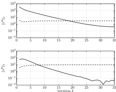
Under assumptions 1 and 2, the ADMM iterates satisfy the following: • Residual convergence. rk→0 as k→ ∞, i.e., the iterates

approach feasibility.

• Objective convergence. f(xk) +g(zk)→p as k→ ∞, i.e., the objective function of the iterates approaches the optimal value.

• Dual variable convergence.yk→y ask→ ∞, wherey is a dual optimal point.

A proof of the residual and objective convergence results is given in appendix A. Note thatxk andzkneed not converge to optimal values, although such results can be shown under additional assumptions.

3.2.2 Convergence in Practice

Simple examples show that ADMM can be very slow to converge to high accuracy. However, it is often the case that ADMM converges to modest accuracy—suﬃcient for many applications—within a few tens of iterations. This behavior makes ADMM similar to algorithms like the conjugate gradient method, for example, in that a few tens of iter-ations will often produce acceptable results of practical use. However, the slow convergence of ADMM also distinguishes it from algorithms such as Newton’s method (or, for constrained problems, interior-point methods), where high accuracy can be attained in a reasonable amount of time. While in some cases it is possible to combine ADMM with a method for producing a high accuracy solution from a low accu-racy solution [64], in the general case ADMM will be practically useful mostly in cases when modest accuracy is suﬃcient. Fortunately, this is usually the case for the kinds of large-scale problems we consider. Also, in the case of statistical and machine learning problems, solving a parameter estimation problem to very high accuracy often yields lit-tle to no improvement in actual prediction performance, the real metric of interest in applications.

(21)

3.3 Optimality Conditions and Stopping Criterion

The necessary and suﬃcient optimality conditions for the ADMM prob-lem (3.1) are primal feasibility,

Ax+Bz −c= 0, (3.8)

and dual feasibility,

0 ∈ ∂f(x) +ATy (3.9)

0 ∈ ∂g(z) +BTy. (3.10) Here, ∂ denotes the subdifferential operator; see, e.g., [140, 19, 99]. (When f and g are differentiable, the subdifferentials ∂f and ∂g can be replaced by the gradients∇f and∇g, and∈can be replaced by =.)

Sincezk+1 minimizes Lρ(xk+1, z, yk) by deﬁnition, we have that

0 ∈ ∂g(zk+1) +BTyk+ρBT(Axk+1+Bzk+1−c) = ∂g(zk+1) +BTyk+ρBTrk+1

= ∂g(zk+1) +BTyk+1.

This means thatzk+1 andyk+1 always satisfy (3.10), so attaining opti-mality comes down to satisfying (3.8) and (3.9). This phenomenon is analogous to the iterates of the method of multipliers always being dual feasible; see page 11.

Sincexk+1 _minimizes _L

ρ(x, zk, yk) by deﬁnition, we have that

0 ∈ ∂f(xk+1) +ATyk+ρAT(Axk+1+Bzk−c) =∂f(xk+1) +AT(yk +ρrk+1+ρB(zk−zk+1)) =∂f(xk+1) +ATyk+1+ρATB(zk−zk+1),

or equivalently,

ρATB(zk+1 −zk)∈∂f(xk+1) +ATyk+1.

This means that the quantity

sk+1=ρATB(zk+1 −zk)

can be viewed as a residual for the dual feasibility condition (3.9). We will refer to sk+1 as the dual residual at iteration k+ 1, and to

(22)

3.3 Optimality Conditions and Stopping Criterion 19 In summary, the optimality conditions for the ADMM problem con-sist of three conditions, (3.8–3.10). The last condition (3.10) always holds for (xk+1, zk+1, yk+1); the residuals for the other two, (3.8) and (3.9), are the primal and dual residuals rk+1 and sk+1, respectively. These two residuals converge to zero as ADMM proceeds. (In fact, the convergence proof in appendix A showsB(zk+1 −zk) converges to zero, which impliessk _{converges to zero.)}

3.3.1 Stopping Criteria

The residuals of the optimality conditions can be related to a bound on the objective suboptimality of the current point, i.e., f(xk) +g(zk)−

p. As shown in the convergence proof in appendix A, we have

f(xk) +g(zk)−p≤ −(yk)Trk+ (xk−x)Tsk. (3.11) This shows that when the residuals rk and sk are small, the objective suboptimality also must be small. We cannot use this inequality directly in a stopping criterion, however, since we do not know x. But if we guess or estimate that xk−x2≤d, we have that

f(xk) +g(zk)−p≤ −(yk)Trk+dsk2≤ yk2rk2+dsk2.

The middle or righthand terms can be used as an approximate bound on the objective suboptimality (which depends on our guess ofd).

This suggests that a reasonable termination criterion is that the primal and dual residuals must be small,i.e.,

rk2≤pri and sk2≤dual, (3.12) wherepri_>_{0 and}dual_>_{0 are feasibility tolerances for the primal and} dual feasibility conditions (3.8) and (3.9), respectively. These tolerances can be chosen using an absolute and relative criterion, such as

pri = √p abs +relmax{Axk2,Bzk2,c2}, dual = √n abs+relATyk2,

where abs >0 is an absolute tolerance and rel>0 is a relative toler-ance. (The factors√pand√naccount for the fact that the2norms are inRpandRn, respectively.) A reasonable value for the relative stopping

(23)

criterion might be rel= 10−3 or 10−4, depending on the application. The choice of absolute stopping criterion depends on the scale of the typical variable values.

3.4 Extensions and Variations

Many variations on the classic ADMM algorithm have been explored in the literature. Here we brieﬂy survey some of these variants, organized into groups of related ideas. Some of these methods can give superior convergence in practice compared to the standard ADMM presented above. Most of the extensions have been rigorously analyzed, so the convergence results described above are still valid (in some cases, under some additional conditions).

3.4.1 Varying Penalty Parameter

A standard extension is to use possibly diﬀerent penalty parametersρk

for each iteration, with the goal of improving the convergence in prac-tice, as well as making performance less dependent on the initial choice of the penalty parameter. In the context of the method of multipliers, this approach is analyzed in [142], where it is shown that superlinear convergence may be achieved if ρk→ ∞. Though it can be diﬃcult to prove the convergence of ADMM whenρ varies by iteration, the

fixed-ρ theory still applies if one just assumes that ρ becomes fixed after a finite number of iterations.

A simple scheme that often works well is (see,e.g., [96, 169]):

ρk+1 :=        τincrρk ifrk2> µsk2 ρk/τdecr ifsk2> µrk2 ρk otherwise, (3.13)

where µ >1, τincr>1, and τdecr >1 are parameters. Typical choices might be µ= 10 and τincr=τdecr= 2. The idea behind this penalty parameter update is to try to keep the primal and dual residual norms within a factor ofµof one another as they both converge to zero.

The ADMM update equations suggest that large values ofρ place a large penalty on violations of primal feasibility and so tend to produce

(24)

3.4 Extensions and Variations 21 small primal residuals. Conversely, the definition ofsk+1 suggests that small values ofρtend to reduce the dual residual, but at the expense of reducing the penalty on primal feasibility, which may result in a larger primal residual. The adjustment scheme (3.13) inflatesρby τincr when the primal residual appears large compared to the dual residual, and deflates ρ by τdecr when the primal residual seems too small relative to the dual residual. This scheme may also be refined by taking into account the relative magnitudes of pri and dual.

When a varying penalty parameter is used in the scaled form of ADMM, the scaled dual variable uk= (1/ρ)yk must also be rescaled after updating ρ; for example, if ρ is halved, uk should be doubled before proceeding.

3.4.2 More General Augmenting Terms

Another idea is to allow for a diﬀerent penalty parameter for each constraint, or more generally, to replace the quadratic term (ρ/2)r2₂

with (1/2)rTP r, whereP is a symmetric positive deﬁnite matrix. When

P is constant, we can interpret this generalized version of ADMM as standard ADMM applied to a modiﬁed initial problem with the equality constraintsr= 0 replaced withF r= 0, whereFTF =P.

3.4.3 Over-relaxation

In thez- andy-updates, the quantityAxk+1 can be replaced with

αkAxk+1−(1−αk)(Bzk−c),

whereαk∈(0,2) is arelaxation parameter; whenαk>1, this technique is calledover-relaxation, and whenαk<1, it is calledunder-relaxation. This scheme is analyzed in [63], and experiments in [59, 64] suggest that over-relaxation withαk∈[1.5,1.8] can improve convergence.

3.4.4 Inexact Minimization

ADMM will converge even when the x- and z-minimization steps are not carried out exactly, provided certain suboptimality measures

(25)

in the minimizations satisfy an appropriate condition, such as being summable. This result is due to Eckstein and Bertsekas [63], building on earlier results by Gol’shtein and Tret’yakov [89]. This technique is important in situations where thex- orz-updates are carried out using an iterative method; it allows us to solve the minimizations only approx-imately at ﬁrst, and then more accurately as the iterations progress.

3.4.5 Update Ordering

Several variations on ADMM involve performing the x-, z-, and y -updates in varying orders or multiple times. For example, we can divide the variables into kblocks, and update each of them in turn, possibly multiple times, before performing each dual variable update; see,e.g., [146]. Carrying out multiplex- andz-updates before they-update can be interpreted as executing multiple Gauss-Seidel passes instead of just one; if many sweeps are carried out before each dual update, the result-ing algorithm is very close to the standard method of multipliers [17, §3.4.4]. Another variation is to perform an additionaly-update between thex- and z-update, with half the step length [17].

3.4.6 Related Algorithms

There are also a number of other algorithms distinct from but inspired by ADMM. For instance, Fukushima [80] applies ADMM to a dual problem formulation, yielding a ‘dual ADMM’ algorithm, which is shown in [65] to be equivalent to the ‘primal Douglas-Rachford’ method discussed in [57, §3.5.6]. As another example, Zhu et al. [183] discuss variations of distributed ADMM (discussed in §7, §8, and §10) that can cope with various complicating factors, such as noise in the mes-sages exchanged for the updates, or asynchronous updates, which can be useful in a regime when some processors or subsystems randomly fail. There are also algorithms resembling a combination of ADMM and theproximal method of multipliers [141], rather than the standard method of multipliers; see,e.g., [33, 60]. Other representative publica-tions include [62, 143, 59, 147, 158, 159, 42].

(26)

3.5 Notes and References 23 3.5 Notes and References

ADMM was originally proposed in the mid-1970s by Glowinski and Marrocco [86] and Gabay and Mercier [82]. There are a number of other important papers analyzing the properties of the algorithm, including [76, 81, 75, 87, 157, 80, 65, 33]. In particular, the convergence of ADMM has been explored by many authors, including Gabay [81] and Eckstein and Bertsekas [63].

ADMM has also been applied to a number of statistical prob-lems, such as constrained sparse regression [18], sparse signal recov-ery [70], image restoration and denoising [72, 154, 134], trace norm regularized least squares minimization [174], sparse inverse covari-ance selection [178], the Dantzig selector [116], and support vector machines [74], among others. For examples in signal processing, see [42, 40, 41, 150, 149] and the references therein.

Many papers analyzing ADMM do so from the perspective of max-imal monotone operators [23, 141, 142, 63, 144]. Briefly, a wide variety of problems can be posed as finding a zero of a maximal monotone operator; for example, iff is closed, proper, and convex, then the sub-differential operator∂f is maximal monotone, and finding a zero of∂f

is simply minimization off; such a minimization may implicitly contain constraints iff is allowed to take the value +∞. Rockafellar’sproximal point algorithm [142] is a general method for ﬁnding a zero of a max-imal monotone operator, and a wide variety of algorithms have been shown to be special cases, including proximal minimization (see §4.1), the method of multipliers, and ADMM. For a more detailed review of the older literature, see [57,§2].

The method of multipliers was shown to be a special case of the proximal point algorithm by Rockafellar [141]. Gabay [81] showed that ADMM is a special case of a method called Douglas-Rachford split-ting for monotone operators [53, 112], and Eckstein and Bertsekas [63] showed in turn that Douglas-Rachford splitting is a special case of the proximal point algorithm. (The variant of ADMM that per-forms an extra y-update between the x- and z-updates is equiva-lent to Peaceman-Rachford splitting [137, 112] instead, as shown by Glowinski and Le Tallec [87].) Using the same framework, Eckstein

(27)

and Bertsekas [63] also showed the relationships between a number of other algorithms, such as Spingarn’s method of partial inverses [153]. Lawrence and Spingarn [108] develop an alternative framework show-ing that Douglas-Rachford splittshow-ing, hence ADMM, is a special case of the proximal point algorithm; Eckstein and Ferris [64] oﬀer a more recent discussion explaining this approach.

The major importance of these results is that they allow the pow-erful convergence theory for the proximal point algorithm to apply directly to ADMM and other methods, and show that many of these algorithms are essentially identical. (But note that our proof of con-vergence of the basic ADMM algorithm, given in appendix A, is self-contained and does not rely on this abstract machinery.) Research on operator splitting methods and their relation to decomposition algo-rithms continues to this day [66, 67].

A considerable body of recent research considers replacing the quadratic penalty term in the standard method of multipliers with a more general deviation penalty, such as one derived from a Bregman divergence [30, 58]; see [22] for background material. Unfortunately, these generalizations do not appear to carry over in a straightforward manner from non-decomposition augmented Lagrangian methods to ADMM: There is currently no proof of convergence known for ADMM with nonquadratic penalty terms.

(28)

4

General Patterns

Structure in f, g, A, and B can often be exploited to carry out the

x- andz-updates more eﬃciently. Here we consider three general cases that we will encounter repeatedly in the sequel: quadratic objective terms, separable objective and constraints, and smooth objective terms. Our discussion will be written for the x-update but applies to the z -update by symmetry. We express the x-update step as

x+= argmin

x

f(x) + (ρ/2)Ax−v2₂,

wherev=−Bz+c−u is a known constant vector for the purposes of thex-update.

4.1 Proximity Operator

First, consider the simple case whereA=I, which appears frequently in the examples. Then thex-update is

x+= argmin

x

f(x) + (ρ/2)x−v2₂.

As a function of v, the righthand side is denoted prox_f,ρ(v) and is called theproximity operator of f with penalty ρ [127]. In variational

(29)

analysis, ˜ f(v) = inf x f(x) + (ρ/2)x−v2₂

is known as theMoreau envelope orMoreau-Yosida regularization off, and is connected to the theory of the proximal point algorithm [144]. The x-minimization in the proximity operator is generally referred to as proximal minimization. While these observations do not by them-selves allow us to improve the eﬃciency of ADMM, it does tie the

x-minimization step to other well known ideas.

When the functionf is simple enough, thex-update (i.e., the prox-imity operator) can be evaluated analytically; see [41] for many exam-ples. For instance, if f is the indicator function of a closed nonempty convex setC, then the x-update is

x+= argmin

x

f(x) + (ρ/2)x−v2₂= Π_C(v),

where Π_Cdenotes projection (in the Euclidean norm) ontoC. This holds independently of the choice ofρ. As an example, if f is the indicator function of the nonnegative orthantRn₊, we havex+= (v)+, the vector obtained by taking the nonnegative part of each component of v.

4.2 Quadratic Objective Terms

Supposef is given by the (convex) quadratic function

f(x) = (1/2)xTP x+qTx+r,

whereP ∈Sn₊, the set of symmetric positive semideﬁniten×n matri-ces. This includes the cases whenf is linear or constant, by settingP, or both P and q, to zero. Then, assumingP +ρATA is invertible, x+

is an aﬃne function ofv given by

x+= (P +ρATA)−1(ρATv−q). (4.1) In other words, computing the x-update amounts to solving a linear system with positive deﬁnite coeﬃcient matrix P +ρATA and right-hand sideρATv−q. As we show below, an appropriate use of numerical linear algebra can exploit this fact and substantially improve perfor-mance. For general background on numerical linear algebra, see [47] or [90]; see [20, appendix C] for a short overview of direct methods.

(30)

4.2 Quadratic Objective Terms 27 4.2.1 Direct Methods

We assume here that adirect method is used to carry out thex-update; the case when an iterative method is used is discussed in §4.3. Direct methods for solving a linear systemF x=g are based on ﬁrstfactoring

F =F1F2···Fkinto a product of simpler matrices, and then computing x=F−1_b _by _solving _{a sequence of problems of the form} _F

izi =zi−1, where z1=F1−1g and x=zk. The solve step is sometimes also called

a back-solve. The computational cost of factorization and back-solve operations depends on the sparsity pattern and other properties of F. The cost of solving F x=g is the sum of the cost of factoring F and the cost of the back-solve.

In our case, the coefficient matrix isF =P +ρATAand the right-hand side isg=ρATv−q, where P ∈Sn₊ and A∈Rp×n. Suppose we exploit no structure in AorP,i.e., we use generic methods that work for any matrix. We can formF =P +ρATA at a cost ofO(pn2) flops (floating point operations). We then carry out a Cholesky factorization ofF at a cost ofO(n3) flops; the back-solve cost isO(n2). (The cost of formingg is negligible compared to the costs listed above.) When p is on the order of, or more thann, the overall cost isO(pn2). (Whenp is less than n in order, the matrix inversion lemma described below can be used to carry out the update inO(p2n) flops.)

4.2.2 Exploiting Sparsity

WhenA andP are such thatF is sparse (i.e., has enough zero entries to be worth exploiting), much more eﬃcient factorization and back-solve routines can be employed. As an extreme case, if P and A are diagonal n×n matrices, then both the factor and solve costs are

O(n). If P and A are banded, then so is F. If F is banded with bandwidth k, the factorization cost is O(nk2) and the back-solve cost is O(nk). In this case, the x-update can be carried out at a cost

O(nk2), plus the cost of forming F. The same approach works when

P +ρATAhas a more general sparsity pattern; in this case, a permuted Cholesky factorization can be used, with permutations chosen to reduce ﬁll-in.

(31)

4.2.3 Caching Factorizations

Now suppose we need to solve multiple linear systems, say,F x(i)₌_g(i)_,

i= 1, . . . , N, with the same coefficient matrix but different righthand sides. This occurs in ADMM when the parameterρ is not changed. In this case, the factorization of the coefficient matrixF can be computed once and then back-solves can be carried out for each righthand side. Iftis the factorization cost andsis the back-solve cost, then the total cost becomes t+N s instead of N(t+s), which would be the cost if we were to factor F each iteration. As long as ρ does not change, we can factor P +ρATA once, and then use this cached factorization in subsequent solve steps. For example, if we do not exploit any structure and use the standard Cholesky factorization, the x-update steps can be carried out a factornmore efficiently than a naive implementation, in which we solve the equations from scratch in each iteration.

When structure is exploited, the ratio betweent and s is typically less thannbut often still significant, so here too there are performance gains. However, in this case, there is less benefit to ρ not changing, so we can weigh the benefit of varyingρagainst the benefit of not recom-puting the factorization of P +ρATA. In general, an implementation should cache the factorization of P +ρATA and then only recompute it if and when ρ changes.

4.2.4 Matrix Inversion Lemma

We can also exploit structure using thematrix inversion lemma, which states that the identity

(P +ρATA)−1=P−1 −ρP−1AT(I +ρAP−1AT)−1AP−1

holds when all the inverses exist. This means that if linear systems with coefficient matrix P can be solved efficiently, and p is small, or at least no larger thannin order, then thex-update can be computed efficiently as well. The same trick as above can also be used to obtain an efficient method for computing multiple updates: The factorization of I +ρAP−1AT can be cached and cheaper back-solves can be used in computing the updates.

(32)

4.2 Quadratic Objective Terms 29 As an example, suppose thatP is diagonal and thatp≤n. A naive method for computing the update costs O(n3) flops in the first itera-tion andO(n2) flops in subsequent iterations, if we store the factors of

P +ρATA. Using the matrix inversion lemma (i.e., using the righthand side above) to compute the x-update costs O(np2_{) ﬂops, an} improve-ment by a factor of (n/p)2 over the naive method. In this case, the dominant cost is forming AP−1AT_{. The factors of} _I₊_ρAP−1_AT _can

be saved after the first update, so subsequent iterations can be car-ried out at cost O(np) flops, a savings of a factor of p over the first update.

Using the matrix inversion lemma to compute x+ can also make it less costly to vary ρ in each iteration. When P is diagonal, for example, we can compute AP−1AT once, and then form and factor

I +ρkAP−1AT in iterationk at a cost of O(p3) ﬂops. In other words, the update costs an additionalO(np) ﬂops, so ifp2 is less than or equal to n in order, there is no additional cost (in order) to carrying out updates withρ varying in each iteration.

4.2.5 Quadratic Function Restricted to an Aﬃne Set

The same comments hold for the slightly more complex case of a convex quadratic function restricted to an aﬃne set:

f(x) = (1/2)xTP x+qTx+r, domf ={x|F x=g}.

Here,x+is still an aﬃne function ofv, and the update involves solving the KKT (Karush-Kuhn-Tucker) system

P +ρI FT F 0 xk+1 ν + q −ρ(zk−uk) −g = 0.

All of the comments above hold here as well: Factorizations can be cached to carry out additional updates more eﬃciently, and structure in the matrices can be exploited to improve the eﬃciency of the factor-ization and back-solve steps.

(33)

4.3 Smooth Objective Terms

4.3.1 Iterative Solvers

When f is smooth, general iterative methods can be used to carry out the x-minimization step. Of particular interest are methods that only require the ability to compute∇f(x) for a given x, to multiply a vector byA, and to multiply a vector by AT. Such methods can scale to relatively large problems. Examples include the standard gradient method, the (nonlinear) conjugate gradient method, and the limited-memory Broyden-Fletcher-Goldfarb-Shanno (L-BFGS) algorithm [113, 26]; see [135] for further details.

The convergence of these methods depends on the conditioning of the function to be minimized. The presence of the quadratic penalty term (ρ/2)Ax−v2₂tends to improve the conditioning of the problem and thus improve the performance of an iterative method for updating

x. Indeed, one method for adjusting the parameter ρfrom iteration to iteration is to increase it until the iterative method used to carry out the updates converges quickly enough.

4.3.2 Early Termination

A standard technique to speed up the algorithm is to terminate the iterative method used to carry out the x-update (or z-update) early,

i.e., before the gradient of f(x) + (ρ/2)Ax−v2₂ is very small. This technique is justiﬁed by the convergence results for ADMM with inexact minimization in the x- and z-update steps. In this case, the required accuracy should be low in the initial iterations of ADMM and then repeatedly increased in each iteration. Early termination in the x- or

z-updates can result in more ADMM iterations, but much lower cost per iteration, giving an overall improvement in eﬃciency.

4.3.3 Warm Start

Another standard trick is to initialize the iterative method used in the x-update at the solution xk obtained in the previous iteration. This is called a warm start. The previous ADMM iterate often gives a good enough approximation to result in far fewer iterations (of the

(34)

4.4 Decomposition 31 iterative method used to compute the updatexk+1) than if the iterative method were started at zero or some other default initialization. This is especially the case when ADMM has almost converged, in which case the updates will not change signiﬁcantly from their previous values. 4.3.4 Quadratic Objective Terms

Even whenf is quadratic, it may be worth using an iterative method rather than a direct method for thex-update. In this case, we can use a standard (possibly preconditioned) conjugate gradient method. This approach makes sense when direct methods do not work (e.g., because they require too much memory) or whenA is dense but a fast method is available for multiplying a vector by A orAT. This is the case, for example, whenA represents the discrete Fourier transform [90].

4.4 Decomposition

4.4.1 Block Separability

Supposex= (x1, . . . , xN) is a partition of the variablexinto subvectors

and thatf is separable with respect to this partition, i.e.,

f(x) =f1(x1) +···+fN(xN),

wherexi∈Rni and

N

i=1ni=N. If the quadratic term Ax22 is also separable with respect to the partition, i.e., ATA is block diagonal conformably with the partition, then the augmented LagrangianLρ is

separable. This means that thex-update can be carried out in parallel, with the subvectorsxi updated by N separate minimizations.

4.4.2 Component Separability

In some cases, the decomposition extends all the way to individual components ofx,i.e.,

f(x) =f1(x1) +···+fn(xn),

wherefi:R→R, andATA is diagonal. Thex-minimization step can

then be carried out via n scalar minimizations, which can in some cases be expressed analytically (but in any case can be computed very eﬃciently). We will call thiscomponent separability.

(35)

4.4.3 Soft Thresholding

For an example that will come up often in the sequel, considerf(x) =

λx1 (withλ >0) andA=I. In this case the (scalar) xi-update is x+_i := argmin xi λ|xi|+ (ρ/2)(xi−vi)2 .

Even though the first term is not differentiable, we can easily compute a simple closed-form solution to this problem by using subdifferential calculus; see [140,§23] for background. Explicitly, the solution is

x+_i :=Sλ/ρ(vi),

where thesoft thresholding operator S is deﬁned as

Sκ(a) =        a−κ a > κ 0 |a| ≤κ a+κ a <−κ, or equivalently, Sκ(a) = (a−κ)+−(−a−κ)+.

Yet another formula, which shows that the soft thresholding operator is a shrinkage operator (i.e., moves a point toward zero), is

Sκ(a) = (1−κ/|a|)+a (4.2) (for a= 0). We refer to updates that reduce to this form as element-wise soft thresholding. In the language of §4.1, soft thresholding is the proximity operator of the1 norm.

(36)

5

Constrained Convex Optimization

The generic constrained convex optimization problem is minimize f(x)

subject to x∈ C, (5.1)

with variablex∈Rn, where f and C are convex. This problem can be rewritten in ADMM form (3.1) as

minimize f(x) +g(z) subject to x−z= 0,

whereg is the indicator function ofC.

The augmented Lagrangian (using the scaled dual variable) is

Lρ(x, z, u) =f(x) +g(z) + (ρ/2)x−z+u22, so the scaled form of ADMM for this problem is

xk+1 := argmin x f(x) + (ρ/2)x−zk +uk2₂ zk+1 := Π_C(xk+1 +uk) uk+1 := uk+xk+1 −zk+1. 33

(37)

Thex-update involves minimizingf plus a convex quadratic function,

i.e., evaluation of the proximal operator associated with f. The z -update is Euclidean projection onto C. The objective f need not be smooth here; indeed, we can include additional constraints (i.e., beyond those represented byx∈ C) by deﬁningf to be +∞where they are vio-lated. In this case, the x-update becomes a constrained optimization problem overdomf ={x|f(x)<∞}.

As with all problems where the constraint is x−z= 0, the primal and dual residuals take the simple form

rk=xk−zk, sk=−ρ(zk−zk−1).

In the following sections we give some more speciﬁc examples. 5.1 Convex Feasibility

5.1.1 Alternating Projections

A classic problem is to ﬁnd a point in the intersection of two closed nonempty convex sets. The classical method, which dates back to the 1930s, is von Neumann’salternating projectionsalgorithm [166, 36, 21]:

xk+1 := Π_C(zk)

zk+1 := Π_D(xk+1),

where Π_C and Π_D are Euclidean projection onto the sets C and D, respectively.

In ADMM form, the problem can be written as minimize f(x) +g(z) subject to x−z= 0,

where f is the indicator function of C and g is the indicator function ofD. The scaled form of ADMM is then

xk+1 := Π_C(zk−uk)

zk+1 := Π_D(xk+1+uk) (5.2)

uk+1 := uk+xk+1−zk+1,

so both the x and z steps involve projection onto a convex set, as in the classical method. This is exactly Dykstra’s alternating projections

(38)

5.1 Convex Feasibility 35 method [56, 9], which is far more eﬃcient than the classical method that does not use the dual variableu.

Here, the norm of the primal residualxk−zk2 has a nice inter-pretation. Since xk∈ C and zk∈ D, xk−zk2 is an upper bound on dist(C,D), the Euclidean distance betweenC and D. If we terminate with rk2≤pri, then we have found a pair of points, one in C and one inD, that are no more thanprifar apart. Alternatively, the point (1/2)(xk+zk) is no more than a distancepri/2 from bothC andD. 5.1.2 Parallel Projections

This method can be applied to the problem of ﬁnding a point in the intersection ofN closed convex sets A1, . . . ,AN in Rn by running the

algorithm inRnN with

C=A1 × ··· × AN, D={(x1, . . . , xN)∈RnN |x1=x2=···=xN}.

Ifx= (x1, . . . , xN)∈RnN, then projection onto C is

Π_C(x) = (Π_A1(x1), . . . ,ΠAN(xN)),

and projection ontoD is

Π_D(x) = (x, x, . . . , x),

where x= (1/N)N_i₌₁xi is the average of x1, . . . , xN. Thus, each step

of ADMM can be carried out by projecting points onto each of the sets Ai in parallel and then averaging the results:

xk_i+1 := Π_A_i(zk−uk_i) zk+1 := 1 N N i=1 (xk_i+1+uk_i) uk_i+1 := uk_i +xk_i+1−zk+1.

Here the ﬁrst and third steps are carried out in parallel, fori= 1, . . . , N. (The description above involves a small abuse of notation in dropping the indexifromzi, since they are all the same.) This can be viewed as a

special case of constrained optimization, as described in§4.4, where the indicator function ofA1∩ ··· ∩ AN splits into the sum of the indicator

(39)

We note for later reference a simpliﬁcation of the ADMM algorithm above. Taking the average (overi) of the last equation we obtain

uk+1=uk+xk+1−zk,

combined with zk+1=xk+1+uk (from the second equation) we see that uk+1= 0. So after the ﬁrst step, the average of ui is zero. This

means thatzk+1 reduces toxk+1. Using these simpliﬁcations, we arrive at the simple algorithm

xk_i+1 := Π_Ai(xk−uki) uk_i+1 := uk_i + (xk_i+1 −xk+1).

This shows thatuk_i is the running sum of the the ‘discrepancies’xk_i −xk

(assumingu0= 0). The ﬁrst step is a parallel projection onto the sets Ci; the second involves averaging the projected points.

There is a large literature on successive projection algorithms and their many applications; see the survey by Bauschke and Borwein [10] for a general overview, Combettes [39] for applications to image pro-cessing, and Censor and Zenios [31,§5] for a discussion in the context of parallel optimization.

5.2 Linear and Quadratic Programming The standard form quadratic program (QP) is

minimize (1/2)xTP x+qTx

subject to Ax=b, x≥0, (5.3)

with variable x∈Rn; we assume that P ∈Sn₊. When P = 0, this reduces to the standard form linear program (LP).

We express it in ADMM form as

minimize f(x) +g(z) subject to x−z= 0,

where

f(x) = (1/2)xTP x+qTx, domf ={x|Ax=b}

is the original objective with restricted domain and g is the indicator function of the nonnegative orthantRn₊.

(40)

5.2 Linear and Quadratic Programming 37 The scaled form of ADMM consists of the iterations

xk+1 := argmin x f(x) + (ρ/2)x−zk +uk2₂ zk+1 := (xk+1 +uk)+ uk+1 := uk+xk+1 −zk+1.

As described in §4.2.5, the x-update is an equality-constrained least squares problem with optimality conditions

P +ρI AT A 0 xk+1 ν + q−ρ(zk−uk) −b = 0.

All of the comments on eﬃcient computation from§4.2, such as storing factorizations so that subsequent iterations can be carried out cheaply, also apply here. For example, if P is diagonal, possibly zero, the ﬁrst

x-update can be carried out at a cost of O(np2_{) ﬂops, where} _p _{is the} number of equality constraints in the original quadratic program. Sub-sequent updates only costO(np) ﬂops.

5.2.1 Linear and Quadratic Cone Programming

More generally, any conic constraintx∈ K can be used in place of the constraintx≥0, in which case the standard quadratic program (5.3) becomes a quadratic conic program. The only change to ADMM is in thez-update, which then involves projection onto K. For example, we can solve a semideﬁnite program withx∈Sn₊ by projectingxk+1 +uk