HAL Id: hal-01235243
https://hal.inria.fr/hal-01235243
Submitted on 29 Nov 2015
HAL
is a multi-disciplinary open access
archive for the deposit and dissemination of
sci-entific research documents, whether they are
pub-lished or not. The documents may come from
teaching and research institutions in France or
abroad, or from public or private research centers.
L’archive ouverte pluridisciplinaire
HAL
, est
destinée au dépôt et à la diffusion de documents
scientifiques de niveau recherche, publiés ou non,
émanant des établissements d’enseignement et de
recherche français ou étrangers, des laboratoires
publics ou privés.
Penalty-Regulated Dynamics and Robust Learning
Procedures in Games
Pierre Coucheney, Bruno Gaujal, Panayotis Mertikopoulos
To cite this version:
Pierre Coucheney, Bruno Gaujal, Panayotis Mertikopoulos. Penalty-Regulated Dynamics and Robust
Learning Procedures in Games. Mathematics of Operations Research, INFORMS, 2015, 40 (3),
pp.611-633. �10.1287/moor.2014.0687�. �hal-01235243�
AND ROBUST LEARNING PROCEDURES IN GAMES
PIERRE COUCHENEY, BRUNO GAUJAL, AND PANAYOTIS MERTIKOPOULOS
Abstract. Starting from a heuristic learning scheme for N-person games,
we derive a new class of continuous-time learning dynamics consisting of a replicator-like drift adjusted by a penalty term that renders the boundary of the game’s strategy space repelling. These penalty-regulated dynamics are equivalent to players keeping an exponentially discounted aggregate of their on-going payoffs and then using a smooth best response to pick an action based on these performance scores. Owing to this inherent duality, the proposed dynamics satisfy a variant of the folk theorem of evolutionary game theory and they converge to (arbitrarily precise) approximations of Nash equilibria in potential games. Motivated by applications to traffic engineering, we exploit this duality further to design a discrete-time, payoff-based learning algorithm which retains these convergence properties and only requires players to observe their in-game payoffs: moreover, the algorithm remains robust in the presence of stochastic perturbations and observation errors, and it does not require any synchronization between players.
1. Introduction
Owing to the computational complexity of Nash equilibria and related game-theoretic solution concepts, algorithms and processes for learning in games have received considerable attention over the last two decades. Such procedures can be divided into two broad categories, depending on whether they evolve in continuous or discrete time: the former class includes the numerous dynamics for learning and evolution (see e.g. Sandholm[34] for a recent survey), whereas the latter focuses on learning algorithms (such as fictitious play and its variants) for infinitely iterated games – for an overview, seeFudenberg and Levine[11] and references therein.
A key challenge in these endeavors is that it is often unreasonable to assume that players can monitor the strategies of their opponents – or even calculate the payoffs of actions that they did not play. As a result, much of the literature on learning in games focuses on payoff-based schemes that only require players to observe the stream of theirin-gamepayoffs: for instance, the regret-matching procedure ofHart and Mas-Colell[12,13] converges to the set of correlated equilibria (in an empirical, time-average sense), whereas the trial-and-error process of Young [42] guarantees with high probability that players will spend a large proportion of their time near a pure Nash equilibrium (provided that such an equilibrium exists).
The authors are greatly indebted to the associate editor and two anonymous referees for their insightful suggestions, and to M. Bravo and R. Cominetti for many helpful discussions and remarks. This work was supported by the European Commission in the framework of the FP7 Network of Excellence in Wireless COMmunications NEWCOM# (contract no. 318306) and the French National Research Agency (ANR) project NETLEARN (grant no. ANR-13-INFR-004).
1
In this paper, we focus on a reinforcement learning framework in which play-ers score their actions over time based on their observed payoffs and they then employ a smooth best response map (such as logit choice) to determine their ac-tions at the next instance of play. Learning mechanisms of this kind have been investigated in continuous time byBörgers and Sarin[5],Rustichini [33], Hopkins [17], Hopkins and Posch [18], Tuyls et al. [39] and many others: Hopkins [17] in particular showed that in2-player games, the continuous-time dynamics that corre-spond to this learning process may be seen as a variant of the replicator dynamics with an extra penaly term that keeps players from attaining the boundary of the game’s strategy space (see alsoHopkins and Posch[18]). On the other hand, from a discrete-time viewpoint, Leslie and Collins [24] used a Q-learning approach to establish the convergence of the resulting learning algorithm in2-player games un-der minimal information assumptions; in a similar vein, Cominetti et al. [9] and Bravo [7] took a moving-average approach for scoring actions in generalN-player games and provided sufficient convergence conditions for the resulting dynamics. Interestingly, in all these cases, when the learning process converges, it converges to a so-called quantal response equilibrium (QRE) which is a fixed point of a per-turbed best response correspondence – as opposed to the standard notion of Nash equilibrium which is a fixed point of the unperturbed best response map; see e.g. McKelvey and Palfrey[27].
Discrete-time processes of this kind are usually analyzed by means of stochastic approximation (SA) techniques that are used to compare the long-term behavior of the discrete-time process to the corresponding mean-field dynamics in continuous time – for a comprehensive introduction to the subject, see e.g. Benaïm [3] and Borkar [6]. Indeed, there are several conditions which guarantee that a discrete-time process and its continuous counterpart both converge to the same sets, so continuous dynamics are usually derived as the limit of (possibly random) discrete-time processes – cf. the aforementioned works byLeslie and Collins[24],Cominetti et al.[9] andBravo[7].
Contrary to this approach, we descend from the continuous to the discrete and we develop two different learning processes from the same dynamical system (the actual algorithm depends crucially on whether we look at the evolution of the play-ers’ strategies or the performance scores of their actions). Accordingly, the first contribution of our paper is to derive a class of penalty-regulated game dynamics consisting of a replicator-like drift plus a penalty term that keeps players from approaching the boundary of the state space. These dynamics are equivalent to players scoring their actions by comparing their exponentially discounted cumula-tive payoffs over time and then using a smooth best response to pick an action; as such, the class of penalty-regulated dynamics that we consider constitutes the strategy-space counterpart of the Q-learning dynamics of Leslie and Collins [24], Hopkins[17] and Tuyls et al.[39]. Thanks to this link to the replicator dynamics, the dynamics converge to quantal response equilibria in potential games, and we also establish a variant of the folk theorem of evolutionary game theory (Hofbauer and Sigmund[15]). In particular, we show the dynamics’ stability and convergence depends crucially on the discount factor used by the players to score their strategies over time: in the undiscounted case, strict Nash equilibria are the only attracting states, just as in the replicator equation; on the other hand, for positive discount factors, only QRE that are close to strict equilibria remain asymptotically stable.
The second contribution of our paper concerns the implementation of these dy-namics as a learning algorithm with the following desirable properties:
(1) The learning process is distributed and stateless: players update their strategies using only their observed in-game payoffs and no further knowl-edge.
(2) The algorithm retains its convergence properties even if the players’ obser-vations are subject to stochastic perturbations and observation errors (or even if they are not up-to-date).
(3) Updates need not be synchronized – there is no need for a global timer used by all players.
These desiderata are key for the design of robust, decentralized optimization pro-tocols in network and traffic engineering, but they also pose significant challenges. Nonetheless, by combining the long-term properties of the continuous-time dynam-ics with stochastic approximation techniques, we show that players converge to ar-bitrarily precise approximations of strict Nash equilibria whenever the game admits a potential function (cf. Theorem 4.4 and Proposition 4.6). Thus, thanks to the congestion characterization of such games (Monderer and Shapley[30]), we obtain a distributed robust optimization method for a wide class of engineering problems, ranging from traffic routing to wireless communications – see e.g. Altman et al.[1], Mertikopoulos et al.[28] and references therein.
1.1. Paper outline and structure. After a few preliminaries, our analysis proper begins in Section 2 where we introduce our cumulative reinforcement learning scheme and derive the associated penalty-regulated dynamics. Owing to the duality between the players’ mixed strategies and the performance scores of their actions (measured by an exponentially discounted aggregate of past payoffs), we obtain two equivalent formulations: the score-based equation (PRL) and the strategy-based dynamics (PD). In Section 3, we exploit this interplay to derive the long-term convergence properties of the dynamics; finally, Section 4 is devoted to the dis-cretization of the dynamics (PRL) and (PD) and their implementation as bona fide learning algorithms.
1.2. Notational conventions. If S = {sα}nα=0 is a finite set, the real space spanned by Swill be denoted by RS and its canonical basis by{es}s∈S. To avoid drowning in a morass of indices, we will make no distinction between s ∈ S and the corresponding basis vectores ofRS, and we will frequently use the index αto
refer interchangeably to eithersαor eα(writing e.g. xα instead ofxsα). Likewise, if{Sk}k∈K is a finite family of finite sets indexed byk∈K, we will use the
short-hands (αk;α−k) for the tuple(. . . , αk−1, αk, αk+1, . . .)∈QkSk and we will write
Pk
αinstead of
P
α∈Sk.
The set ∆(S) of probability measures on S will be identified with the unit n -dimensional simplex ∆(S) ≡ {x ∈ RS : P
αxα = 1andxα ≥ 0} of RS. Finally,
regarding players and their actions, we will follow the original convention of Nash and employ Latin indices (k, `, . . .) for players, while keeping Greek ones (α, β, . . .) for their actions (pure strategies); also, unless otherwise mentioned, we will use
1.3. Definitions from game theory. A finite game G ≡ G(N,A, u) will be a tuple consisting of a) a finite set of players N = {1, . . . , N}; b) a finite set Ak
of actions (or pure strategies) for each player k ∈ N; and c) the players’ payoff functions uk:A→R, whereA≡QkAk denotes the game’s action space, i.e. the
set of all action profiles (α1, . . . , αN), αk ∈Ak. Arestriction ofGwill then be a
gameG0 ≡G0(N,A0, u0)with the same players asG, each with a subsetA0k ⊆Ak
of their original actions, and with payoff functions u0k ≡uk|A0 suitably restricted
to the reduced action spaceA0=Q
kA
0
k ofG
0.
Of course, players can mix their actions by taking probability distributionsxk=
(xkα)α∈Ak ∈∆(Ak)over their action setsAk. In that case, their expected payoffs will be uk(x) = X1 α1 · · ·XN αN uk(α1, . . . , αN)x1,α1· · ·xN,αN, (1.1) where x = (x1, . . . , xN) denotes the players’ strategy profile and uk(α1, . . . , αN)
is the payoff to player k in the (pure) action profile (α1, . . . , αN) ∈ A;1 more
explicitly, if player k plays the pure strategy α ∈ Ak, we will use the notation
ukα(x)≡uk(α;x−k) = uk(x1, . . . , α, . . . , xN). In this mixed context, the strategy
space of player kwill be the simplex Xk ≡∆(Ak)while the strategy space of the
game will be the convex polytopeX≡Q
kXk. Together with the players’ (expected)
payoff functionsuk:X→R, the tuple(N,X, u)will be called themixed extensionof
Gand it will also be denoted byG(relying on context to resolve any ambiguities). The most prominent solution concept in game theory is that of Nash equilibrium (NE) which characterizes profiles that are resilient against unilateral deviations; formally,q∈Xwill be aNash equilibriumofGwhen
uk(xk;q−k)≤uk(q) for allxk∈Xk and for allk∈N. (NE)
In particular, if (NE) is strict for allxk ∈Xk\ {qk},k∈N,qwill be called astrict
Nash equilibrium; finally, arestricted equilibrium of Gwill be a Nash equilibrium of a restrictionG0 ofG.
An especially relevant class of finite games is obtained when the players’ payoff functions satisfy thepotential property:
ukα(x)−ukβ(x) =U(α;x−k)−U(β;x−k) (1.2)
for some (necessarily) multilinear function U: X → R. When this is the case, the game will be called a potential game with potential function U, and as is well known, the pure Nash equilibria of G will be precisely the vertices of X that are local maximizers ofU (Monderer and Shapley[30]).
2. Reinforcement learning and penalty-regulated dynamics Our goal in this section will be to derive a class of learning dynamics based on the following reinforcement premise: agents keep a long-term “performance score” for each of their actions and they then use a smooth best response to map these scores to strategies and continue playing. Accordingly, our analysis will comprise two components:
(1) The assessment stage (Section 2.1) describes the precise way with which players aggregate past payoff information in order to update their actions’ performance scores.
1Recall that we will be usingαfor both elementsα∈A
kand basis vectorseα ∈∆(Ak), so
(2) The choice stage (Section 2.2) then details how these scores are used to select a mixed strategy.
For simplicity, we will work here in continuous time and we will assume that players can observe (or otherwise calculate) the payoffs of all their actions in a given strategy profile; the descent from continuous to discrete time and the effect of imperfect information will be explored in Section4.
2.1. The assessment stage: aggregation of past information. The aggrega-tion scheme that we will consider is the familiar exponential discounting model:
ykα(t) =
Z t
0
λt−sukα(x(s))ds, (2.1)
where λ ∈ (0,∞) is the model’s discount rate, x(s) ∈ X is the players’ strategy profile at time sand we are assuming for the moment that the model is initially unbiased, i.e. y(0) = 0. Clearly then:
(1) For λ∈(0,1) the model assigns exponentially more weight to more recent observations.
(2) If λ = 1 all past instances are treated uniformly – e.g. as in Rustichini [33],Hofbauer et al.[16],Sorin[37],Mertikopoulos and Moustakas[29] and many others.
(3) For λ > 1, the scheme (2.1) instead assigns exponentially more weight to older instances.
With this in mind, differentiating (2.1) readily yields
˙
ykα =ukα−T ykα, (2.2)
where
T ≡log(1/λ) (2.3)
represents thediscount rate of the performance assessement scheme (2.1). In tune with our previous discussion, the standard exponential discounting regimeλ∈(0,1)
corresponds to positiveT >0, a discount rate of 0means that past information is not penalized in favor of more recent observations, while T < 0 means that past observations are reinforced in favor of more recent ones.
Remark 1. Leslie and Collins[24] and Tuyls et al. [39] examined the aggregation scheme (2.2) from a quite different viewpoint, namely as the continuous-time limit of theQ-learning estimator
ykα(n+ 1) =ykα(n) +γn+1(ukα(x(n))−ykα(n))×
1(αk(n+ 1) =α) P(αk(n+ 1) =α|Fn)
, (2.4) where1andPdenote respectively the indicator and probability of playerkchoosing
α∈Ak at timen+ 1 given the historyFn of the process up to timen, whileγn is
a variable step-size withP
nγn= +∞andPnγ
2
n <+∞(see also Fudenberg and
Levine[11]). The exact interplay between (2.2) and (2.4) will be explored in detail in Section4; for now, we simply note that (2.2) can be interpreted both as a model of discounting past information and also as a movingQ-average.
Remark 2. We should also note here the relation between (2.4) and the moving average estimator ofCominetti et al.[9] that omits the factorP(αk(n+ 1) =α|Fn)
(or the similar estimator ofBravo [7] which has a state-dependent step size). As a result of this difference, the mean-field dynamics ofCominetti et al.[9] are scaled by
xkα, leading to the adjusted dynamicsy˙kα =xkα(ukα−ykα). Given this difference
in form, there is essentially no overlap between our results and those ofCominetti et al.[9], but we will endeavor to draw analogies with their results wherever possible. 2.2. The choice stage: smooth best responses. Having established the way that agents evaluate their strategies’ performance over time, we now turn to map-ping these assessment scores to mixed strategies x ∈ X. To that end, a natural choice would be for each agent to pick the strategy with the highest score via the mapping
yk7→arg maxxk∈Xk
Pk
βxkβykβ (2.5)
Nevertheless, this “best response” approach carries several problems: First, if two scoresykαandykβ happen to be equal (e.g. if there are payoff ties), (2.5) becomes
a multi-valued mapping which requires a tie-breaking rule to be resolved (and is theoretically quite cumbersome to boot). Additionally, such a practice could lead to completely discontinuous trajectories of play in continuous time – for instance, if the payoffs ukα are driven by an additive white Gaussian noise process, as is
commonly the case in information-theoretic applications of game theory; see e.g. Altman et al.[1]. Finally, since best responding generically leads to pure strategies, such a process precludes convergence of strategies to non-pure equilibria in finite games.
To circumvent these obstacles, we will replace the arg max operator with the regularized variant Qk(yk) = arg maxxk∈Xk n Pk βxkβykβ−hk(xk) o , (2.6)
where hk:Xk → R is a smooth strongly convex function which acts as a penalty
(or “control cost”) to the maximization objective Pk
βxkβykβ of player k.2 Choice
models of this type are known in the literature assmooth best response maps (or quantal response functions) and have seen extensive use in game-theoretic learning; for a comprehensive account, see e.g. van Damme [40], McKelvey and Palfrey [27], Fudenberg and Levine[11],Hofbauer and Sandholm [14], Sandholm[34] and references therein. Formally, followingAlvarez et al.[2], we have:
Definition 2.1. LetSbe a finite set and let∆≡∆(S)be the unit simplex spanned byS. We will say thath: ∆→R∪ {+∞} is apenalty function on∆ if:
(1) his finite except possibly on the relative boundarybd(∆)of∆.
(2) h is continuous on ∆, smooth on rel int(∆), and |dh(x)| → +∞ when x
converges tobd(∆).
(3) his convex on∆ and strongly convex onrel int(∆).
2Note here that this penalty mechanism is different than the penalty imputed to past payoff observations in the performance assessment step (2.1): (2.1) discounts past instances of play whereas (2.6) discourages the player from choosing pure strategies. Despite this fundamental difference, these two processes end up being intertwined in the resulting learning scheme, so we will use the term “penalty” for both mechanisms, irrespective of origin.
We will also say that h is (regularly) decomposable with kernel θ if h(x) can be written in the form:
h(x) =X
β∈Sθ(xβ) (2.7)
whereθ: [0,+1]→R∪ {+∞} is a continuous function such that a) θis finite and smooth on(0,1].
b) θ00(x)>0 for allx∈(0,1].
c) limx→0+θ0(x) =−∞and limx→0+θ0(x)/θ00(x) = 0.
In this context, the mapQ:RS→∆of (2.6) will be referred to as thechoice map (orsmooth best response orquantal response function) induced byh.
Given that (2.6) allows us to view Q(ηy) = arg maxx∈∆{
P
βxβyβ−η−1h(x)}
as a smooth approximation to thearg maxoperator in the limitη → ∞(i.e. when the penalty term becomes negligible), the choice stage of our learning process will consist precisely of the choice maps that are derived from penalty functions as above; for simplicity of presentation however, our analysis will mostly focus on the decomposable case.
In any event, Definition2.1 will be central to our considerations, so some com-ments are in order:
Remark 1. The fact that choice maps are well-defined and single-valued is an imme-diate consequence of the convexity and boundary properties ofh; the smoothness of
Qthen follows from standard arguments in convex analysis – see e.g. Chapter 26 in Rockafellar [32]. Moreover, the requirementlimx→0+θ0(x)/θ00(x) = 0of Definition 2.1is just a safety net to ensure that penalty functions do not exhibit pathological traits near the boundarybd(∆)of∆. As can be easily seen, this growth condition is satisfied by all of the example functions (2.8) below; in fact, to go beyond this natural requirement,θ00 must oscillate deeply and densely near0.
Remark 2. Examples of penalty functions abound; some of the most prominent ones are:
1. The Gibbs entropy: h(x) =P
βxβlogxβ. (2.8a)
2. The Tsallis entropy: h(x) = (1−q)−1P
β(xβ−xqβ), 0< q≤1. (2.8b)
3. The Burg entropy: h(x) =−P
βlogxβ. (2.8c)
Strictly speaking, the Tsallis entropy is not well-defined forq= 1, but it approaches the standard Gibbs entropy asq→1, so we will use (2.8a) forq= 1in that case.3 Example 1 (Logit choice). The most well-known example of a smooth best response is the so-calledlogit map
Gα(y) =
exp(yα)
P
βexp(yβ)
, (2.9)
which is generated by the Gibbs entropyh(x) =P
βxβlogxβ of (2.8a). For uses
of this map in game-theoretic learning, see e.g. Cominetti et al. [9], Fudenberg and Levine [11], Hofbauer and Sandholm [14], Hofbauer et al. [16], Leslie and Collins[24],McFadden[26], Marsili et al.[25],Mertikopoulos and Moustakas [29], Rustichini[33], Sorin[37] and many others.
3Actually, entropies are concave in statistical physics and information theory, but this detail will not concern us here.
Remark 3. Interestingly,McKelvey and Palfrey [27] provide an alternative deriva-tion of (2.9) as follows: assume first that the score vectory is subject to additive stochastic fluctuations of the form
˜
yα=yα+ξα, (2.10)
where theξαare independent Gumbel-distributed random variables with zero mean
and scale parameter ε >0 (amounting to a variance ofε2π2/6). It is then known that thechoice probability Pα(y)of theα-th action (defined as the probability that
αmaximizes the perturbed variabley˜α) is just
Pα(y)≡P(˜yα= maxβy˜β) =Gα(ε−1y). (2.11)
As a result, the logit map can be seen as either a smooth best response to the deterministic penalty functionh(x)or as a perturbed best response to the stochastic perturbation model (2.10); furthermore, both models approximate the ordinary best response correspondence when the relative magnitude of the perturbations approaches 0. In a more general context, Hofbauer and Sandholm [14] showed that this observation continues to hold even when the stochastic perturbationsξα
are not Gumbel-distributed but follow an arbitrary probability law with a strictly positive and smooth density function: mutatis mutandis, the choice probabilities of a stochastic perturbation model of the form (2.10) can be interpreted as a smooth best response map induced by a deterministic penalty function in the sense of Definition2.1.
2.3. The dynamics of penalty-regulated learning. Combining the results of the previous two sections, we will focus on thepenalty-regulated learning process:
ykα(t) =ykα(0)e−T t+ Z t 0 e−T(t−s)ukα(x(s))ds, xk(t) =Qk(yk(t)), (PRL)
where ykα(0) represents the initial bias of player k towards action α∈ Ak,4 T is
the model’s discount rate, andQk:RAk→Xk is the smooth best response map of
playerk (induced in turn by some player-specific penalty functionhk:Xk→R).
From an implementation perspective, the difficulty with (PRL) is twofold: First, it is not always practical to write the choice maps Qk in a closed-form expression
that the agents can use to update their strategies.5 Furthermore, even when this is possible, (PRL) is a two-step, primal-dual process which does not allow agents to update their strategies directly. The rest of this section will thus be devoted to writing (PRL) as a continuous-time dynamical system onXthat can be updated with minimal computation overhead.
To that end, we will focus on decomposable penalty functions of the form
hk(xk) =
Xk
βθk(xkβ), (2.12)
4The exponential decay ofy(0)is perhaps best explained by the differential formulation (2.2) for whichy(0)is an initial condition; in words, the player’s initial bias simply dies out at the same rate as a payoff observation att= 0.
5The case of the Gibbs entropy is a shining (but, ultimately, misleading) exception to the norm.
where the kernels θk, k ∈ N, satisfy the convexity and steepness conditions of
Definition 2.1.6 In this context, the Karush–Kuhn–Tucker (KKT) conditions for the maximization problem (2.6) give
ykα−θ0k(xkα) =ζk, (2.13)
where ζk is the Lagrange multiplier for the equality constraintP k
αxkα = 1.7 By
differentiating, we then obtain:
˙
ykα−θk00(xkα) ˙xkα = ˙ζk, (2.14)
and hence, a little algebra yields:
˙ xkα= 1 θ00 k(xkα) ˙ ykα−ζ˙k = 1 θ00k(xkα) ukα(x)−T ykα−ζ˙k = 1 θ00k(xkα) ukα(x)−T θ0k(xkα)− ζ˙k+T ζk, (2.15)
where the second equality follows from the definition of the penalty-regulated scheme (PRL) and the last one from the KKT equation (2.13). However, since
Pk
αxkα = 1, we must also have P k
αx˙kα = 0; thus, summing (2.15) overα ∈Ak
gives: ˙ ζk+T ζk = Θ00k(xk) Xk β 1 θ00 k(xkβ) [ukβ(x)−T θk0(xkβ)], (2.16)
whereΘ00k denotes the harmonic aggregate:8
Θ00k(xk) = Xk β1/θ 00 k(xkβ) −1 . (2.17)
In this way, by putting everything together, we finally obtain thepenalty-regulated dynamics ˙ xkα= 1 θ00k(xkα) ukα(x)−Θ00k(xk) Xk β ukβ(x) θk00(xkβ) (PD) − T θ00 k(xkα) θk0(xkα)−Θ00k(xk) Xk β θ0k(xkβ) θ00(x kβ) , (2.18)
Along with the aggregation-driven learning scheme (PRL), the dynamics (PD) will be the main focus of our paper, so some remarks and examples are in order: Example 2 (The Replicator Dynamics). As a special case, the Gibbs kernelθ(x) = xlogxof (2.8a) leads to theadjusted replicator equation
˙ xkα=xkα ukα(x)− Xk βxkβukβ(x) −T xkα logxkα− Xk βxkβlogxkβ . (RDT)
6Non-decomposablehcan be treated similarly but the end expression is more cumbersome so we will not present it.
7The complementary slackness multipliers for the inequality constraintsx
kα≥0can be omitted
because the steepness properties ofθkensure that the solution of (2.6) is attained in the interior
of the simplex.
8Needless to say,Θ00
h is not a second derivatives per se; we just use this notation for visual
As the name implies, when the discount rate T vanishes, (RDT) freezes to the
ordinary (asymmetric) replicator dynamics ofTaylor and Jonker[38]:
˙ xkα=xkα ukα(x)− Xk βxkβukβ(x) . (RD)
In this way, forT = 0, we recover the well-known equivalence between the replicator dynamics and exponential learning in continuous time – for a more detailed treat-ment, see e.g. Rustichini [33], Hofbauer et al. [16], Sorin [37] and Mertikopoulos and Moustakas[29].
Remark 4 (Links with existing dynamics). Leslie and Collins [24] derived a dif-ferential version of the penalty-regulated learning process (PRL) as the mean-field dynamics of the Q-learning estimator (2.4); independently, Tuyls et al. [39] ob-tained a variant of the strategy-space dynamics (PD) in the context ofQ-learning in2-player games. A version of (PD) for2-player games also appeared inHopkins [17] andHopkins and Posch[18] as a perturbed reinforcement learning model; other than that however, the penalty-regulated dynamics (PD) appear to be new.
Interestingly, in terms of structure, the differential system (PD) consists of a replicator-like term driven by the game’s payoffs, plus a game-independent adjust-ment term which reflects the penalty imputed to past payoffs. This highlights a certain structural similarity between (PD) and other classes of game dynamics with comparable correction mechanisms: for instance, in a stochastic setting, Itô’s lemma leads to a “second order in space” correction in the stochastic replicator dynamics ofFudenberg and Harris[10],Cabrales[8], andMertikopoulos and Moustakas[29]; likewise, such terms also appear in the “second order in time” approach of Laraki and Mertikopoulos[20,21].
The reason for this similarity is that all these models are first defined in terms of a set of auxiliary variables: absolute population sizes in Fudenberg and Harris [10] andCabrales[8], and payoff scores inLaraki and Mertikopoulos[20] and here. Differentiation of these “dual” variables with respect to time yields a replicator-like term (which carries the dependence on the game’s payoffs) plus a game-independent adjustment which only depends on the relation between these “dual” variables and the players’ mixed strategies (the system’s “primal” variables).
Remark 5 (Well-posedness). Importantly, the dynamics (PD) arewell-posed in the sense that they admit unique global solutions for every interior initial condition
x(0) ∈ rel int(X). Since the vector field of (PD) is not Lipschitz, perhaps the easiest way to see this is by using the integral representation (PRL) of the dynamics: indeed, given that the payoff functions ukα are Lipschitz and bounded, the scores
ykα(t)will remain finite for allt≥0, so interior solutions x(t) =Q(y(t))of (PD)
will be defined for allt≥0.
Moreover, even though the dynamics (PD) are technically defined only on the relative interior of the game’s strategy space, the steepness and regularity require-ments of Definition2.1allow us to extend the dynamics to the boundary bd(X)of
Xby continuity (i.e. by writing1/θ00(xkα) =θ0(xkα)/θ00(xkα) = 0whenxkα= 0).
By doing just that, every subfaceX0 ofXwill be forward invariant under (PD), so the class of penalty-regulated dynamics may be seen as a subclass of the imitative dynamics introduced byBjörnerstedt and Weibull[4] (see alsoWeibull[41]).
Remark 6 (Sharpened choices). In addition to tuning the discount rate of the learn-ing scheme (PRL), players can also sharpen their smooth best response model by replacing the choice stage (2.6) with
xk=Qk(ηkyk) (2.19)
for someηk >0. The choice parametersηk may thus be viewed as (player-specific)
inverse temperatures: as ηk → ∞, the choice map of player kfreezes down to the
arg max operator, whereas in the limit ηk →0, playerk will tend to mix actions
uniformly, irrespectively of their performance scores.
In this context, the same reasoning as before leads to the rate-adjusted dynamics:
˙ xkα= ηk θ00k(xkα) ukα(x)−Θ00k(xk) Xk β ukβ(x) θk00(xkβ) (PDη) − T θ00 k(xkα) θk0(xkα)−Θ00k(xk) Xk β θ0k(xkβ) θ00(x kβ) . (2.20)
We thus see that the parameters T and η play very different roles in (PDη): the
discount rateT affects only the game-independent penalty term of (PDη) whereas
ηk affects only the term which is driven by the game’s payoffs.
3. Long-run rationality analysis
In this section, our aim will be to analyze the asymptotic properties of the penalty-regulated dynamics (PD) with respect to standard game-theoretic solution concepts. Thus, in conjunction with the notion of Nash equilibrium, we will also focus on the widely studied concept ofquantal response equilibria:
Definition 3.1(McKelvey and Palfrey[27]). LetG≡G(N,A, u)be a finite game and assume that each player k∈ N is endowed with a quantal response function
Qk:RAk → Xk (cf. Definition 2.1). We will say that q = (q1, . . . , qN) ∈ X is a
quantal response equilibrium(QRE) ofGwith respect toQ(or aQ-equilibrium for short) when, for someρ≥0 and for allk∈N:
qk=Qk(ρuk(q)), (QRE)
where uk(q) = (ukα(q))α∈Ak ∈ RA
k denotes here the payoff vector of player k. More generally, we will say that q∈X is arestricted QRE of Gif it is a QRE of some restrictionG0 ofG.
The scale parameter ρ ≥ 0 will be called the rationality level of the QRE in question. Obviously, whenρ= 0, QRE have no ties to the game’s payoffs; at the other end of the spectrum, when ρ → ∞, quantal response functions approach best responses and the notion of a QRE approximates smoothly that of a Nash equilibrium. To see this in more detail, let q∗ ∈ X be a Nash equilibrium of G, and let γ:U → X be a smooth curve on X defined on a half-infinite interval of the form U = [a,+∞), a ∈ R. We will then say that γ is a Q-path to q∗ when
γ(ρ) is a Q-equilibrium of G with rationality levelρ and limρ→∞γ(ρ) = q∗; in a
similar vein, we will say that q ∈ X is a Q-approximation of q∗ when q is itself a Q-equilibrium and there is a Q-path joining q to q∗ (van Damme [40] uses the terminologyapproachable).
H0, 0L H3, 1L H1, 3L H0, 0L 0.0 0.2 0.4 0.6 0.8 1.0 0.0 0.2 0.4 0.6 0.8 1.0 x y
Penalty-Adjusted Replicator DyanmicsHT=2L
H0, 0L H3, 1L H1, 3L H0, 0L 0.0 0.2 0.4 0.6 0.8 1.0 0.0 0.2 0.4 0.6 0.8 1.0 x y
Penalty-Adjusted Replicator DyanmicsHT=0.93L
H0, 0L H3, 1L H1, 3L H0, 0L 0.0 0.2 0.4 0.6 0.8 1.0 0.0 0.2 0.4 0.6 0.8 1.0 x y
Penalty-Adjusted Replicator DyanmicsHT=0.5L
H0, 0L H3, 1L H1, 3L H0, 0L 0.0 0.2 0.4 0.6 0.8 1.0 0.0 0.2 0.4 0.6 0.8 1.0 x y
Penalty-Adjusted Replicator DyanmicsHT=0.1L
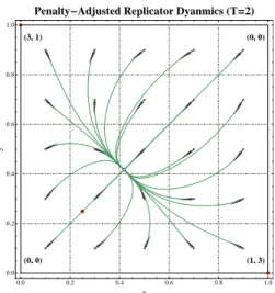
Figure 1. Phase portraits of the penalty-adjusted replicator dynamics (RDT) in a2×2 potential game (Nash equilibria are depicted in dark red
and interior rest points in light/dark blue; for the game’s payoffs, see the ver-tex labels). For high discount ratesT 0, the dynamics fail to keep track of the game’s payoffs and their only rest point is a global attractor which ap-proaches the barycenter ofXasT →+∞(corresponding to a QRE of very low rationality level). As the players’ discount rate drops down to the critical valueTc ≈0.935, the globally stable QRE becomes unstable and undergoes
a supercritical pitchfork bifurcation (a phase transition) which results in the appearance of two asymptotically stable QRE that approach the strict Nash equilibria of the game asT →0+.
Example 3. By far the most widely used specification of a QRE is thelogit equilib-rium which corresponds to the Gibbs choice map (2.9): in particular, we will say that q∈Xis a logit equilibrium ofGwhenqkα = exp(ρukα(q))/Pβexp(ρukβ(q))
3.1. Stability analysis. We begin by linking the rest points of (PD) to the game’s QRE:
Proposition 3.2. LetG≡G(N,A, u)be a finite game and assume that each player
k∈Nis endowed with a quantal response functionQk:RAk →Xk Then:
(1) ForT >0, the rest points of the penalty-regulated dynamics (PD)coincide with the restricted QRE ofGwith rationality levelρ= 1/T.
(2) ForT = 0, the rest points of (PD)are the restricted Nash equilibria ofG. Proof. Proof. Since the proposition concerns restricted equilibria, it suffices to establish our assertion for interior rest points; given that the faces ofXare forward-invariant under the dynamics (PD), the general claim follows by descending to an appropriate restrictionG0 ofG.
To wit, (PD) implies that any interior rest pointq∈rel int(X)will haveukα(q)−
T θ0k(qkα) =ukβ(q)−T θ0k(qkβ)for allα, β∈Ak and for allk∈N. As such, ifT = 0,
we will have ukα(q) =ukβ(q) for all α, β ∈ Ak, i.e. q will be a Nash equilibrium
of G; otherwise, for T >0, a comparison with the KKT conditions (2.13) implies thatq is the (unique) solution of the maximization problem:
qk = arg maxxk∈Xk n Xk βxkβukβ(xk;q−k)−T hk(xk) o = arg maxx k∈Xk n Xk βxkβ·T −1u kβ(xk;q−k)−hk(xk) o =Qk T−1uk(q) , (3.1) i.e. qis aQ-equilibrium of Gwith rationality levelρ= 1/T. Proposition3.2shows that the discount rateTof the dynamics (PD) plays a dou-ble role: on the one hand, it determines the discount rate of the players’ assessment phase (2.2), so it reflects the importance that players give to past observations; on the other hand,T also determines the rationality level of the rest points of (PD), measuring how far the stationary points of the players’ learning process are from being Nash. That being said, stationarity does not capture the long-run behavior of a dynamical system, so the rest of our analysis will be focused on the asymptotic properties of (PD). To that end, we begin with the special case of potential games where the players’ payoff functions are aligned along a potential function in the sense of (1.2); in this context, the game’s potential function is “almost” increasing along the solution orbits of (PD) ifT is small enough:
Lemma 3.3. LetG≡G(N,A, u)be a finite game with potentialU and assume that each player k∈ N is endowed with a decomposable penalty functionhk:Xk →R.
Then, the function
F(x)≡T X
k∈N
hk(xk)−U(x) (3.2)
is Lyapunov for the penalty-regulated dynamics (PD): for any interior orbitx(t)of (PD), we have dtdF(x(t))≤0 with equality if and only ifx(0)is a QRE of G. Proof. Proof. By differentiatingF, we readily obtain:
∂F ∂xkα
where θk is the kernel of the penalty function of player k and we have used the
potential property (1.2) of G to write ∂x∂U
kα = ukα. Hence, for any interior orbit
x(t)of (PD), some algebra yields:
dF dt = X k Xk α ∂F ∂xkα ˙ xkα =−X k Xk α 1 θ00(x kα) (T θ0k(xkα)−ukα(x)) 2 +X kΘ 00 k(xk) Xk α 1 θ00k(xkα) (T θk0(xkα)−ukα(x)) 2 =−X k 1 Θ00k(xk) " Xk απkαw 2 kα− Xk απkαwkα 2# , (3.4)
where we have set πkα = Θ00k(xkα)/θ00k(xkα) andwkα =T θk0(xkα)−ukα(x). Since
πkα≥0andP k
απkα = 1by construction, our assertion follows by Jensen’s
inequal-ity (simply note that the conditionwkα =wkβ for allα, β∈Ak is only satisfied at
the QRE ofG).
Needless to say, Lemma3.3can be easily extended to orbits lying in any subface
X0ofXby considering the game’s restricted QRE. Indeed, given that the restricted
QRE ofGthat are supported in a subfaceX0ofXcoincide with the local minimizers ofF|X0, Lemma3.3gives:
Proposition 3.4. Let x(t) be a solution orbit of the penalty-regulated dynamics (PD) for a potential gameG. Then:
(1) ForT >0,x(t)converges to a restricted QRE of Gwith the same support asx(0).
(2) For T = 0, x(t) converges to a restricted Nash equilibrium with support contained in that ofx(0).
Proposition 3.4implies that interior solutions of (PD) forT > 0can only con-verge to interior points in potential games; as we show below, this behavior actually applies toany finite game:
Proposition 3.5. Let x(t) be an interior solution orbit of the penalty-regulated dynamics (PD)forT >0. Then, any ω-limit ofx(t)is interior; in particular, the boundarybd(X)of Xrepels all interior orbits.9
Proof. Proof. Our proof will be based on the integral representation (PRL) of the penalty-regulated dynamics (PD). Indeed, with ukα bounded onX(say by some
M >0), we get: |ykα(t)| ≤ |ykα(0)|e−T t+ Z t 0 e−T(t−s)|ukα(x(s))| ds ≤ |ykα(0)|e−T t+ M T 1−e −T t , (3.5) so anyω-limit of (PRL) must lie in the rectangleCT =Q
kC T k where C T k ={yk∈ RAk : |y
kα| ≤ M/T}. However, since Qk maps RAk to rel int(Xk) continuously,
Qk(CkT)will be a compact set contained inrel int(Xk), and our assertion follows by
recalling thatx(t) =Q(y(t)).
The above highlights an important connection between the score variables ykα
and the players’ mixed strategy shares xkα: the asymptotic boundedness of the
scores implies that the solution orbits of (PD) will be repelled by the boundary
bd(X) of the game’s strategy space. On the other hand, this connection is not a two-way street because the smooth best response map Qk:RAk →Xk is not a
diffeomorphism: Qk(y) =Qk(y+c(1, . . . ,1)) for everyc ∈R, soQk collapses the
directions that are parallel to(1, . . . ,1).
To obtain a diffeomorphic set of score-like variables, let Ak ={αk,0, αk,1, . . .} denote the action set of playerk and consider therelative scores:
zkµ=θ0k(xkµ)−θk0(xk,0) =ykµ−yk,0, µ= 1,2, . . . , (3.6) where the last equality follows from the KKT conditions (2.13). In words, zkµ
simply measures the score difference between the µ-th action of playerk and the “flagged” 0-th action; as such, the evolution ofzkµ over time will be:
˙
zkµ= ˙ykµ−y˙k,0=ukµ−T ykµ−(uk,0−T yk,0) = ∆ukµ−T zkµ, (3.7)
where∆ukµ=ukµ−uk,0. In particular, these relative scores remain unchanged if a players’ payoffs are offset by the same amount, a fact which is reflected in the following:
Lemma 3.6. Let Ak,0 =Ak\ {αk,0} = {αk,1, αk,2, . . .}. Then, with notation as above, the map ιk:xk7→zk is a diffeomorphism fromrel int(Xk)toRAk,0.
Proof. Proof. We begin by showing that ιk is surjective. Indeed, let zk ∈ RAk,0
and set yk = (0, zk,0, zk,1, . . .). Then, if xk =Qk(yk), the KKT conditions (2.13)
become −θ0k(xk,0) = ζk and zkµ −θk0(xkµ) = ζk for all µ ∈ Ak,0. This gives
zkµ=θ0k(xkµ)−θ0k(xk,0)for allµ∈Ak,0, i.e. ιk is onto.
Assume now that θ0k(xkµ)−θk0(xkµ) = θ0k(x
0 kµ)−θ 0 k(x 0 k,0) for some xk, x0k ∈
rel int(Xk). A trivial rearrangement givesθk0(xkα)−θk0(x
0 kα) =θ 0 k(xkβ)−θ0k(x 0 kβ)
for all α, β ∈ Ak, so there exists some ξk ∈ Rsuch that θ0k(x
0
kα) = ξk +θk0(xkα)
for all α ∈ Ak. With θ0k strictly increasing, this implies that x0kα > xkα (resp.
x0kα< xkα, resp. x0kα =xkα) for allα∈Ak ifξk >0(resp. ξk <0, resp. ξk= 0).
However, given that the components of xk and x0k both sum to 1, we must have
x0kα=xkα for allαi.e. the mapxk7→zk is injective.
Now, treating xk,0 = 1−Pµ∈Ak,0xkµ as a dependent variable, the Jacobian matrix ofιk will be:
Jµνk = ∂zkµ ∂xkν =θk00(xkµ)δµν+θ0k 1−P µ∈Ak,0xkµ . (3.8)
Then, lettingθkµ00 =θ00k(xkµ)andθk,000=θk0
1−Pk
µxkµ
, it is easy to see thatJk µν
is invertible with inverse matrix
Jkµν= δµν θ00kµ −
Θ00k
where Θ00 k = P α∈Ak1/θ 00 kα −1
. Indeed, dropping the index k for simplicity, a simple inspection gives:
X ν6=0 JµνJνρ= X ν6=0 θµ00δµν+θ000 · δνρ/θν00−Θ 00/(θ00 νθ 00 ρ) =X ν6=0 θµ00δµνδνρ/θν00+θ 00 0δνρ/θ00ν−θ 00 µΘ 00δ µν/(θ00νθ 00 ρ)−θ 00 0Θ 00/(θ00 νθ 00 ρ) =δµρ+θ000/θ00ρ−Θ00/θ00ρ−θ000Θ00 X ν6=0 1(θν00θρ00) =δµρ. (3.10)
The above shows thatιk is a smooth immersion; sinceιk is bijective, it will also be
a diffeomorphism by the inverse function theorem, and our proof is complete. With this diffeomorphism at hand, we now show that the penalty-regulated dynamics (PD) are contracting ifT >0(a result which ties in well with Proposition 3.5above):
Proposition 3.7. LetK0⊆rel int(X)be a compact set of interior initial conditions and let Kt={x(t) :x(0)∈K0} be its evolution under the dynamics (PD). Then, there exists a volume formVolonrel int(X)such that
Vol(Kt) = Vol(K0) exp(−T A0t), (3.11) where A0 = Pk(card(Ak)−1). In other words, the penalty-regulated dynamics
(PD) are incompressible forT= 0 and contracting forT >0.
Proof. Proof. Our proof will be based on the relative score variables zkµ of (3.6).
Indeed, letU0 be an open set of QkRAk,0 and let Wkµ= ∆ukµ(x)−T zkµ denote
the RHS of (3.7). Liouville’s theorem then gives
d
dtVol0(Ut) = Z
Ut
divW dΩ0, (3.12)
where dΩ0 =Vk,µdzkµ is the ordinary Euclidean volume form on QkRAk,0, Vol0 denotes the associated (Lebesgue) measure onQ
kRAk,0andUtis the image ofU0at timetunder (3.7). However, given that∆ukµdoes not depend onzk(recall thatukµ
anduk,0 themselves do not depend on xk), we will also have ∂W∂zkµ
kµ =−T. Hence, summing over allµ∈Ak,0andk∈N, we obtaindivW =−Pk(card(Ak)−1)T =
−A0T and (3.12) yieldsVol(Ut) = Vol(U0) exp(−A0T t).
In view of the above, letι= (ι1, . . . , ιN) : rel int(X)→QkRAk,0 be the product
of the “relative score” diffeomorphisms of Lemma3.6, and let Vol =ι∗Vol0 be the pullback of the Euclidean volumeVol0(·)on QkRAk,0 to rel int(X), i.e. Vol(K) =
Vol0(ι(K))for any (Borel)K⊆rel int(X). Then, lettingU0=ι(K0), our assertion follows from the volume evolution equation above and the fact thatι(x(t))solves
(3.7) wheneverx(t)solves (PD).
When applied to (RDT) for T = 0, Proposition 3.7 yields the classical result
that the asymmetric replicator dynamics (RD) are incompressible – and thus do not admit interior attractors (Hofbauer and Sigmund[15],Ritzberger and Weibull [31]).10 We thus see that incompressibility characterizes a much more general class
10This does not hold in the symmetric case because the symmetrized payoffu
α(x)depends on
of dynamics: in our learning context, it simply reflects the fact that players weigh their past observations uniformly (neither discounting, nor reinforcing them).
That said, in the case of the replicator dynamics, we have a significantly clearer picture regarding the stability and attraction properties of a game’s equilibria; in particular, the folk theorem of evolutionary game theory (Hofbauer and Sigmund [15]) states that:11
(1) If an interior trajectory converges, its limit is Nash. (2) If a state is Lyapunov stable, then it is also Nash.
(3) A state is asymptotically stable if and only if it is a strict Nash equilibrium. By comparison, in the context of the penalty-regulated game dynamics (PD), we have:
Theorem 3.8. Let G≡G(N,A, u) be a finite game, let hk:Xk →Rbe a
decom-posable penalty function for each playerk∈N, and letQk:RAk→Xk denote each
player’s choice map. Then, the penalty-regulated dynamics (PD)have the following properties:
(1) ForT >0, ifq∈Xis Lyapunov stable then it is also a QRE ofG; moreover, ifqis aQ-approximate strict Nash equilibrium andT is small enough, then
q is also asymptotically stable.
(2) ForT = 0, ifq∈Xis Lyapunov stable, then it is also a Nash equilibrium of G; furthermore,q is asymptotically stable if and only if it is a strict Nash equilibrium ofG.
Proof. Proof. Our proof will be broken up in two parts depending on the discount rateT of (PD):
The caseT >0. LetT >0 and assume thatq∈Xis Lyapunov stable (and, hence, stationary). Clearly, ifqis interior, it must also be a QRE ofGby Proposition3.2, so there is nothing to show. Suppose therefore thatq∈bd(X); then, by Proposition 3.5, we may pick a neighborhoodU ofqinXsuch thatcl(U)does not contain any
ω-limit points of the interior ofXunder (PD). However, sinceqis Lyapunov stable, any interior solution that is wholly contained in U must have anω-limit in cl(U), a contradiction.
Regarding the asymptotic stability of Q-approximate strict equilibria, assume without loss of generality that q∗= (α1,0, . . . , αN,0)is a strict Nash equilibrium of Gand letq≡q(T)∈Xbe aQ-approximation ofq∗with rationality levelρ= 1/T. Furthermore, letWkµ= ∆ukµ−T zkµand consider∆ukµ as a function of onlyx`µ,
µ∈A`,0, by treatingx`,0= 1−Pµx`µ as a dependent variable. Then, as in the
proof of Lemma3.6, a simple differentiation yields:
∂Wkµ ∂z`ν q = −T if`=k,ν =µ, 0 if`=k,ν 6=µ, P ρ∈A`,0J νρ ` (q) ∂ ∂w`ρ∆ukµ otherwise, (3.13)
whereJ`νρ(q)denotes the inverse Jacobian matrix (3.9) of the mapx7→zevaluated atq.
11Recall thatq∈Xis said to beLyapunov stable(orstable) when for every neighborhoodUof
qinX, there exists a neighborhoodV ofqinXsuch that ifx(0)∈V thenx(t)∈Ufor allt≥0;
qis calledattractingwhen there exists a neighborhoodU ofqinXsuch thatlimt→∞x(t) =qif x(0)∈U; finally,qis calledasymptotically stablewhen it is both stable and attracting.
We will show that all the elements of (3.13) with` 6=k or µ 6=ν are of order
o(T)as T →0+, so (3.13) is dominated by the diagonal elements ∂Wkµ
∂zkµ =−T for
small T. To do so, it suffices to show thatT−1J`νρ →+∞ as T → 0+; however, sinceqis aQ-approximation of the strict equilibriumq∗= (α1,0, . . . , αN,0), we will also have qkµ ≡ qkµ(T) → q∗kµ = 0 and qk,0 → qk,∗0 = 1 as T → 0
+. Moreover, recalling that q is a QRE of G with rationality level ρ = 1/T, we will also have
∆ukµ(q) =T θ0(qkµ)−T θ0(qk,0), implying in turn thatT θ0(qkµ(T))→∆ukµ(q∗)<0
asT →0+. We thus obtain: 1 T θ00(q kµ(T)) = θ 0(q kµ(T)) θ00(q kµ(T)) 1 T θ0(q kµ(T)) → 0 ∆ukµ(q∗) = 0, (3.14)
and hence, on account of (3.9) and (3.14), we will have J`νρ =o(T) for small T. By continuity, the eigenvalues of (3.13) evaluated atq≡q(T)will all be negative if
T >0is small enough, soqwill be a hyperbolic rest point of (3.7); by the Hartman-Grobman theorem it will then also be structurally stable, and hence asymptotically stable as well.
The caseT = 0. ForT = 0, letqbe Lyapunov stable so that every neighborhoodU
ofqinXadmits an interior orbitx(t)that stays inUfor allt≥0; we then claim that
q is Nash. Indeed, assume ad abusrdum thatαk,0 ∈supp(q)hasuk,0(q)< ukµ(q)
for someµ∈Ak,0≡Ak\ {αk,0}, and letU be a neighborhood ofqsuch thatxk,0>
qk,0/2 and ∆ukµ(x)≥ m >0 for all x∈ U. Picking an orbit x(t)that is wholly
contained inU, the dynamics (3.7) readily givezkµ(t)≥zk,0(0) +mt, implying in turn thatzkµ(t)→+∞as t→ ∞. However, withzkµ =θ0(xkµ)−θ0(xk,0), this is only possible ifxkµ(t)→0, a contradiction.
Assume now thatq= (α1,0, . . . , αN,0)is a strict Nash equilibrium ofG. To show that q is Lyapunov stable, it will be again convenient to work with the relative scores zkµ and show that if m ∈ Ris sufficiently negative, then every trajectory
z(t)that starts in the open setUm={z∈QkRAk,0 :zkµ< m}always stays inUm;
sinceUmmaps viaι−1: QkRAk,0 →rel int(X)to a neighborhood ofqinrel int(X),
this is easily seen to imply Lyapunov stability forqin X.
In view of the above, pick m∈Rso that ∆ukµ(x(z))≤ −ε <0 for all z ∈Um
and letτm= inf{t:z(t)∈/ Um}be the time it takesz(t)to escapeUm. Then, ifτm
is finite andt≤τm, the relative score dynamics (3.7) readily yield
zkµ(t) =zkµ(0)+
Z t
0
∆ukµ(Q0(z(s)))ds≤zkµ(0)−εt < m for allµ∈Ak,0, k∈N.
(3.15) Thus, substitutingτm fortin (3.15), we obtain a contradiction to the definition of
τmand we conclude thatz(t)always stays inUmifmis chosen negative enough –
i.e. qis Lyapunov stable.
To show thatq is in addition attracting, it suffices to let t→ ∞ in (3.15) and recall the definition (3.6) of thezkµvariables. Finally, for the converse implication,
assume thatqis not pure; in particular, assume thatqlies in the relative interior of a non-singleton subfaceX0spanned bysupp(q). Proposition3.7shows thatqcannot attract a relatively open neighborhoodU0 of initial conditions inX0 because (PD) remains volume-preserving when restricted to any subface X0 of X. This implies thatq cannot be attracting inX, soqcannot be asymptotically stable either.
In conjunction with our previous results, Theorem 3.8 provides an interesting insight into the role of the dynamics’ discount rate T: for small T > 0, the dy-namics (PD) are attracted to the interior of X and can only converge to points that are approximately Nash; on the other hand, for T = 0, the solutions (PD) are only attracted to strict Nash equilibria (see also Fig.1). As such, Theorem3.8 and Proposition 3.4suggest that if one seeks to reach a (pure) Nash equilibrium, the best convergence properties are provided by the “no discounting” case T = 0. Nonetheless, as we shall see in the following section, if one seeks to implement the dynamics (PD) as a bona fide learning algorithm in discrete time, the “positive discounting” regimeT >0is much more robust than the “no disounting” case – all the while allowing players to converge arbitrarily close to a Nash equilibrium. 3.2. The case T < 0: reinforcing past observations. In this section, we ex-amine briefly what happens when players use a negative discount rate T <0, i.e. they reinforce past observations instead of discounting them. As we shall see, even though the form of the dynamics (PRL)/(PD) remains the same (the derivation of (PRL) and (PD) does not depend on the sign ofT), their properties are quite different in the regimeT <0.
The first thing to note is that the definition of a QRE also extends to negative rationality levels ρ < 0 that describe an “anti-rational” behavior where players attempt to minimize their payoffs: indeed, the QRE of a gameG≡G(N,A, u)for negativeρare simply QRE of the opposite game−G≡(N,A,−u), and asρ→ −∞, these equilibria approximate the Nash equilibria of−G.
In this way, repeating the analysis of Section3.1, we obtain:
Theorem 3.9. Let G≡G(N,A, u)be a finite game and assume that each player
k∈N is endowed with a decomposable penalty function hk:Xk →R with induced
choice mapQk:RAk →Xk. Then, in the case of a negative discount rateT <0:
(1) The rest points of the penalty-regulated dynamics (PD)are the restricted QRE of the opposite game−G.
(2) The dynamics (PD)are expanding with respect to the volume form of Proposi-tion3.7and (3.11)continues to hold.
(3) A strategy profileq∈Xis asymptotically stable if and only if it is pure (i.e. a vertex ofX); any other rest point of (PD)is unstable.
Theorem3.9will be our main result forT <0, so some remarks in order: Remark 7. The gamesG and −G have the same restricted equilibria, so the rest points of (PD) for smallT >0(corresponding to QRE with largeρ= 1/T →+∞) transition smoothly to perturbed equilibria with small T <0 (ρ→ −∞) via the “fully rational” case T = 0(which corresponds to the Nash equilibria of the game whenρ=±∞). In fact, by continuity, the phase portrait of the dynamics (PD) for sufficiently smallT (positive or negative) will be broadly similar to the base case
T = 0(at least, in the generic case where there are no payoff ties inG). The main difference between positive and negative discount rates is that, for small T < 0, the orbits of (PD) are attracted to the vertices ofX(though each individual vertex might have a vanishingly small basin of attraction), whereas for smallT > 0, the dynamics are only attracted to interior points (which, however, are arbitrarily close to the vertices ofX).
H0, 0L H3, 1L H1, 3L H0, 0L 0.0 0.2 0.4 0.6 0.8 1.0 0.0 0.2 0.4 0.6 0.8 1.0 x y
Penalty-Adjusted Replicator DyanmicsHT=0.25L
H0, 0L H3, 1L H1, 3L H0, 0L 0.0 0.2 0.4 0.6 0.8 1.0 0.0 0.2 0.4 0.6 0.8 1.0 x y
Penalty-Adjusted Replicator DynamicsHT=-1.5L
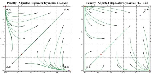
Figure 2. Phase portraits of the penalty-adjusted replicator dynamics (RDT) showing the transition from positive to negative discount rates in the
game of Fig. 1. For smallT >0, the rest points of (PD) areQ-approximate Nash equilibria (red dots), and they attract almost all interior solutions; asT
drops to negative values, the non-equilibrium vertices ofXbecome asymptoti-cally stable (but with a small basin of attraction), and each one gives birth to an unstable QRE of the opposite game in a subcritical pitchfork bifurcation. Of these two equilibria, the one closer to the game’s interior Nash equilibrium is annihilated with the pre-existing QRE atT ≈ −0.278, and asT→ −∞, we obtain a time-inverted image of theT→+∞portrait with the only remaining QRE repelling all trajectories towards the vertices ofX; Figure2(b)shows the case where only one (repelling) rest point remains.
Remark 8. It should be noted that the expanding property of (PD) forT <0does not clash with the fact that the vertices of X are asymptotically stable. Indeed, as can be easily seen by Lemma3.6, sets of unit volume become vanishingly small (in the Euclidean sense) near the boundary bd(X) of X; as such, the expanding property of the dynamics (PD) precludes the existence of attractors in the interior ofX, but not of boundary attractors.12
Proof. Proof of Theorem3.9. The time inversion t7→ −tin (PD) is equivalent to the inversionu7→ −u,T 7→ −T, so our first claim follows from theT >0 part of Proposition 3.2; likewise, our second claim is obtained by noting that the proof of Proposition 3.7does not differentiate between positive and negative temperatures either.
For the last part, our proof will be based on the dynamics (3.7); more precisely, focus for convenience on the vertex q = (α1,0, . . . , αN,0) of X, and let Ak,0 =
Ak\ {αk,0} as usual. Then, a simple integration of (3.7) yields
zkµ(t) =zkµ(0)e−T t+
Z t
0
e−T(t−s)∆ukµ(x(s))ds. (3.16)
12Obviously, the same applies to every subfaceX0 ofX, explaining in this way why only the vertices ofXare attracting.
However, given that∆ukµ is bounded onX(say by some M >0), the last integral
will be bounded in absolute value byM|T|−1 e|T|t−1, and hence:
zkµ(t)≤ −M|T|−1+ zkµ(0) +M|T|−1 e|T|t. (3.17) Thus, if we pick zkµ(0) < −M|T|− 1
, we will have limt→∞zkµ(t) = −∞ for all
µ ∈ Ak,0, k ∈ N, i.e. x(t) → q. Accordingly, given that the set UT = {z ∈
Q
kRAk,0 :zkµ<−M|T|−
1
} is just the image of a neighborhood ofqin rel int(X)
under the diffeomorphism of Lemma3.6,qwill attract all nearby interior solutions of (PD); by restriction, this property applies to any subface ofXwhich containsq, soq is attracting. Finally, ifzkµ(0)<−M|T|
−1
, we will also havezkµ(t)< zkµ(0)
for allt≥0 (cf. the proof of Proposition 3.5), soq is Lyapunov stable, and hence asymptotically stable as well.
Conversely, assume that q ∈ X is a non-pure Lyapunov stable state; then, by descending to a subface of X if necessary, we may assume that q is interior. In that case, ifU is a neighborhood ofqin rel int(X), Proposition3.7shows that any neighborhoodV ofqthat is contained inU will eventually grow to a volume larger than that ofU under (PD), so there is no open set of trajectories contained inU. This shows that only vertices ofXcan be stable, and our proof is complete.
4. Discrete-time learning algorithms
In this section, we examine how the dynamics (PRL) and (PD) may be used for learning in finite games that are played repeatedly over time. To that end, a first-order Euler discretization of the dynamics (PRL) gives the recurrence
Ykα(n+ 1) =Ykα(n) +γ[ukα(X(n))−T Ykα(n)],
Xk(n+ 1) =Q(Yk(n+ 1)),
(4.1) which is well-known to track (PRL) arbitrarily well over finite time horizons when the discretization stepγ is sufficiently small. That said, in many practical scenar-ios, players cannot monitor the mixed strategies of their opponents, so (4.1) cannot be updated directly. As a result, in the absence of perfect monitoring (or a simi-lar oracle-like device), any distributed discretization of the dynamics (PRL)/(PD) should involve only the players’ observed payoffs and no other information.
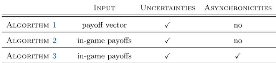
In what follows (cf. Table 1 for a summary), we will drop such information and coordination assumptions one by one: in Algorithm 1, players will only be assumed to possess a bounded, unbiased estimate of their actions’ payoffs; this assumption is then dropped in Algorithm2 which only requires players to observe their in-game payoffs (or a perturbed version thereof); finally, Algorithm3provides a decentralized variant of Algorithm 2 where players are no longer assumed to update their strategies in a synchronous way.
4.1. Stochastic approximation of continuous dynamics. We begin by recall-ing a few general elements from the theory of stochastic approximation. Followrecall-ing Benaïm[3] andBorkar[6], letSbe a finite set, and letZ(n),n∈N, be a stochastic process inRS such that
Z(n+ 1) =Z(n) +γn+1U(n+ 1), (4.2) whereγnis a sequence of step sizes andU(n)is a stochastic process inRSadapted to
Input Uncertainties Asynchronicities
Algorithm 1 payoff vector X no
Algorithm 2 in-game payoffs X no
Algorithm 3 in-game payoffs X X
Table 1. Summary of the information and coordination requirements of the learning algorithms of Section4.
we will say that (4.2) is a stochastic approximation of the dynamical system
˙
z=f(z), (MD)
if E[U(n+ 1)|Fn] = f(Z(n))for all n. More explicitly, if we split the so-called
innovation term U(n)of (4.2) into its average valuef(Z(n)) =E[U(n+ 1)|Fn]and
a zero-mean noise termV(n+ 1) =U(n+ 1)−f(Z(n)), (4.2) takes the form
Z(n+ 1) =Z(n) +γn+1[f(Z(n)) +V(n+ 1)], (SA) which is just a noisy Euler-like discretization of (MD); conversely, (MD) will be referred to as themean dynamics of the stochastic recursion (SA).
The main goal of the theory of stochastic approximation is to relate the process (SA) to the solution trajectories of the mean dynamics (MD). Some standard assumptions that enable this comparison are:
(A1) The step sequenceγnis(`2−`1)–summable, viz. Pnγn=∞andPnγ
2
n<∞.
(A2) V(n)is a martingale difference withsupnEhkV(n+ 1)k2 Fn
i <∞. (A3) The stochastic processZ(n)is bounded: supnkZ(n)k<∞(a.s.).
Under these assumptions, the next lemma provides a sufficient condition which ensures that (SA) converges to the set of stationary points of (MD):
Lemma 4.1. Assume that the dynamics (MD) admit a strict Lyapunov function (i.e. a real-valued function which decreases along non-stationary orbits of (MD)) such that the set of values taken by this function at the rest points of (MD) has measure zero inR. Then, under Assumptions(A1)–(A3)above, every limit point of the stochastic approximation process (SA)belongs to a connected set of rest points of the mean dynamics (MD).
Proof. Proof. Our claim is a direct consequence of the following string of results inBenaïm [3]: Prop. 4.2, Prop. 4.1, Theorem 5.7, and Prop. 6.4. As an immediate application of Lemma4.1, letGbe a finite game with potential
U. By Lemma3.3, the functionF=T h−Uis Lyapunov for (PRL)/(PD); moreover, sinceU is multilinear andhis smooth and strictly convex, Sard’s theorem (Lee[22]) ensures that the set of values taken by F at its critical points has measure zero. Thus, any stochastic approximation of (PRL)/(PD) which satisfies Assumptions (A1)–(A3) above can only converge to a connected set of restricted QRE.
4.2. Score-based learning. In this section, we present an algorithmic implemen-tation of the score-based learning dynamics (PRL) under two different information assumptions: first, we will assume that players possess an unbiased estimate for the payoff of each of their actions (including those that they did not play at a given instance); we will then drop this assumption and describe the issues that arise when players can only observe their in-game payoffs.
4.2.1. Learning with imperfect payoff estimates. If the players can estimate the payoffs of actions that they did not play, the sequence of play will be as follows:
(1) At stage n+ 1, each player selects an actionαk(n+ 1) ∈Ak based on a
mixed strategyXk(n)∈Xk.
(2) Every player receives a bounded and unbiased estimate uˆkα(n+ 1) of his
actions’ payoffs, viz.
(a) E[ˆukα(n+ 1)|Fn] =ukα(X(n)),
(b) |uˆkα(n+ 1)| ≤C(a.s.),
whereFnis the history of the process up to stagenandC >0is a constant.
(3) Players choose a mixed strategyXk(n+ 1)∈Xk and the process repeats.
It should be noted here that players are not explicitly assumed to monitor their opponents’ strategies, nor to communicate with each other in any way: for instance, in congestion and resource allocation games, players can compute their out-of-game payoffs by probing the game’s facilities for a broadcast. That said, the specifics of how such estimates can be obtained will not concern us here: in what follows, we only seek to examine how players can exploit such information when it is available. To that end, the score-based learning process (PRL) gives:
Algorithm 1Score-based learning with imperfect payoff monitoring
n←0;
foreachplayer k∈Ndo
initializeYk∈RAk and setXk←Qk(Yk); # initialization
Repeat
n←n+ 1;
foreachplayerk∈Ndosimultaneously
select new actionαk∈Ak according to mixed strategy Xk; # choose action
foreachplayerk∈Ndo foreachactionα∈Ak do
observeuˆkα; # estimate payoff of each action
Ykα←Ykα+γn(ˆukα−T Ykα); # update score of each action
Xk ←Qk(Yk); # update mixed strategy
until termination criterion is reached
To study the convergence properties of Algorithm1, letYk(n)denote the score
vector of player k at the n-th iteration of the algorithm – and likewise for the player’s mixed strategyXk(n)∈Xk, chosen actionαk(n)∈Ak and payoff estimates
ˆ
ukα(n)∈R. Then, for allk∈Nandα∈Ak, we get:
E[(Ykα(n+ 1)−Ykα(n))/γn+1|Fn] =E[ˆukα(n+ 1)|Fn]−T Ykα(n)
=ukα(X(n))−T Ykα(n). (4.3)
Together with the choice ruleXk(n) =Qk(Yk(n)), the RHS of (4.3) yields the score
dynamics (PRL), so the process X(n) generated by Algorithm 1 is a stochastic approximation of (PRL). We thus get:
Theorem 4.2. Let G be a potential game. If the step size sequence γn satisfies
(A1) and the players’ payoff estimatesuˆkα are bounded and unbiased, Algorithm1
converges (a.s.) to a connected set of QRE ofGwith rationality parameterρ= 1/T. In particular,X(n)converges withinε(T)of a Nash equilibrium ofGand the error
ε(T)vanishes asT →0.
Proof. Proof. In view of the discussion following Lemma4.1, we will establish our claim by showing that Assumptions (A1)–(A3) are all satisfied in the case of the stochastic approximation
Ykα(n+ 1) =Ykα(n) +γn+1[ˆukα(n+ 1)−T Ykα(n)]. (4.4)
Assumption (A1) is true by design, so there is nothing to show. Furthermore, expressing the noise term of (4.4) asVkα(n+1) = ˆukα(n+1)−ukα(X(n)), we readily
obtainE[Vkα(n+ 1)|Fn] = 0andE V2 kα(n+ 1) Fn ≤2C2, so Assumption (A2) also holds. Finally, withuˆkαbounded (a.s.),Ykαwill also be bounded (a.s.): indeed,
note first that0≤1−T γn ≤1for allnlarger than somen0; then, using the uniform norm for convenience of notation, the iterates of (4.4) will satisfy kY(n+ 1)k ≤ (1−T γn+1)kY(n)k+γn+1C for all sufficiently largen. Hence:
(1) If kY(n)k ≤ C/T, we will also have kY(n+ 1)k ≤ (1−T γn+1)C/T +
γn+1C=C/T.
(2) If kY(n)k > C/T, we will have kY(n+ 1)k ≤ kY(n)k −T γn+1kY(n)k+
γn+1C≤ kY(n)k, i.e. kYkdecreases.
The above shows thatkY(n)kis bounded byT−1C∨max
n≥n0kY(n)k, so Assump-tion (A3) also holds. By ProposiAssump-tion3.2and the discussion following Lemma4.1, we then conclude thatX(n)converges to a connected set ofrestrictedQRE ofG. How-ever, sinceY(n)is bounded,X(n)will be bounded away from the boundarybd(X)
ofXbecause the image of a compact set underQis itself compact inrel int(X). As such, any limit point ofX(n)will be interior and our claim follows. 4.2.2. The issue with in-game observations. Assume now that the only information at the players’ disposal is the payoff of their chosen actions, possibly perturbed by some random noise process. Formally, ifαk(n+ 1)denotes the action of playerkat
the(n+ 1)-th stage of the process, we will assume that the corresponding observed payoff is of the form
ˆ
uk(n+ 1) =uk(α1(n+ 1), . . . , αN(n+ 1)) +ξk(n+ 1), (4.5)
where the noise process ξk is a bounded, F-adapted martingale difference (i.e. E[ξk(n+ 1)|Fn] = 0 and kξkk ≤ C for some C > 0) with ξk(n+ 1)
indepen-dent ofαk(n+ 1).13
13These assumptions are rather mild and can be easily justifed by invoking the independence between the nature-driven perturbations to the players’ payoffs and the sampling done by each player to select an action at each stage. In fact, this accounts not only for i.i.d. perturbations