Robust Wilks' Statistic based on RMCD for One-Way Multivariate Analysis of Variance (MANOVA)

(1)

Robust Wilks' Statistic based on RMCD for One-Way

Multivariate Analysis of Variance (MANOVA)

Abdullah A. Ameen and Osama H. Abbas

Department of Mathematics, College of Science, University of Basra, Basra, Iraq.

Abstract

The classical Wilks' statistic is the most using for testing the hypotheses of equal mean vectors of several multivariate normal populations for one-way MANOVA. It is extremely sensitive to the influence of outliers. Therefore, the robust Wilks' statistic based on reweighted minimum covariance determinant (RMCD) estimator with Hampel weighted function has been proposed. The distribution of the proposed statistic differs from the classical one.

Mont Carlo simulations are used to evaluate the performance of the test statistic under the normal and contaminated distribution for the data set. Moreover, the type I error rate and power of test have been considered as statistical measures to comparison between the classical and the robust statistics.

The results show that, the robust Wilks' statistic based on RMCD is closely to the classical Wilks' statistic in case of normal distribution for the data set while in case of contaminated distribution the method in question is the best.

Keywords: One-Way Multivariate Analysis of Variance, Wilks' Statistic, Outliers, Robustness, Minimum Covariance Determinant Estimator.

1 Introduction

One-way multivariate analysis of variance (MANOVA) deals with testing the hypothesis of equal mean vectors of several multivariate normal groups. The classical Wilks' statistic is the most using for testing the hypotheses in the one-way MANOVA. Under the classical assumptions that all groups arise from multivariate normal distributions, many test statistics are extremely sensitive to the influence of outliers (Beak and Cook (1983)). Thus, in order to reduce the influence of outliers, the robust statistics have been proposed. In the one-group, the Hotelling's statistic is the standard tool for inference about the center of a multivariate normal distribution, Willems et al. (2002) proposed the robust Hotelling's statistic based on the minimum covariance determinant (MCD) estimator. Meral Candan and Serpil Aktas (2003) implemented the robust Hotelling's statistic based on the minimum volume ellipsoid (MVE) estimator to test the hypothesis about the location parameter of one group. In the two groups, Ameen (2007) suggested the robust Hotelling's statistic based on the reweighted minimum covariance determinant (RMCD) estimator to test a hypothesis about equal two mean vectors. Van Aelst and Willems (2011) proposed a robust Wilks' statistic for test the hypotheses in the one-way MANOVA based on S and the MM-estimators.

The effect of outliers on the classical Wilks' statistic will be illustrated in the simulation study in Section 4. Therefore we proposed robust estimators instead of the classical ones for computing Wilks' statistic. For this purpose, the minimum covariance determinant (MCD) estimator that proposed by Rousseeuw in 1985 which is a highly robust estimators of location and scatter are used. Thus, the MCD estimator is summarized in section 3. In order to increase the efficiency while retaining high robustness, one can apply reweighted estimators for the MCD estimator. In section 2, we constructed the robust Wilks' statistic differs from the classical one. Monte Carlo simulations are used to evaluate the performance of the proposed test statistic under various distributions in terms of the simulated significance level, power of the test and

(2)

2 The Robust Wilks' Statistic

To formalize the hypotheses in one-way multivariate analysis of variance (MANOVA), let us assumed that there are many of independent random groups, say 𝑘 groups, for every sample there are 𝑛𝑘 multivariate normal observations 𝐲𝑖𝑗 , 𝑖 = 1, 2, ⋯ , 𝑘 , 𝑗 = 1, 2, ⋯ , 𝑛𝑖 of 𝑝 dimension with mean vector 𝜇𝑖 and equal covariance matrix ∑. Then, the null and alternative hypotheses can be written as:

𝐻0∶ 𝝁1= 𝝁2= ⋯ = 𝝁𝑘 𝐻1∶ 𝝁𝑖≠ 𝝁𝑗 𝑓𝑜𝑟 𝑎𝑡 𝑙𝑎𝑒𝑠𝑡 𝑜𝑛𝑒 𝑜𝑓 𝑖 ≠ 𝑗

There are many of statistics used for testing 𝐻0, one of the most widely used is Wilks' statistic Λ

which is defined as (Rencher (2002)):

Λ = |𝐸|

|𝐸 + 𝐻| … (1)

where 𝐻 and 𝐸 are the "between" and "within" of 𝑝 × 𝑝 matrices, respectively, have formulas:

𝐻 = ∑ 𝑛𝑖(𝐲̅𝑖 ∙− 𝐲̅∙ ∙) 𝑘 𝑖=1 (𝐲̅𝑖 ∙− 𝐲̅∙ ∙)𝑡, 𝐸 = ∑ ∑(𝐲𝑖 𝑗− 𝐲̅𝑖 ∙) 𝑛_𝑖 𝑗=1 (𝐲𝑖 𝑗− 𝐲̅𝑖 ∙) 𝑡 𝑘 𝑖=1 where 𝐲̅𝑖 ∙= 1 𝑛𝑖 ∑ 𝐲𝑖 𝑗 𝑛𝑖 𝑗=1 , 𝐲̅∙ ∙= 1 𝑛∑ ∑ 𝐲𝑖 𝑗 𝑛𝑖 𝑗=1 𝑘 𝑖=1 , 𝑛 = ∑ 𝑛𝑖 𝑘 𝑖=1

The null hypothesis 𝐻0 is reject if Λ ≤ Λ𝛼,𝑝,𝑣_𝑒,𝑣_ℎwhere Λ𝛼,𝑝,𝑣_𝑒,𝑣_ℎ is the exact critical values for Wilks' table with level of significance 𝛼 and degrees of freedom 𝑝, 𝑣𝑒 and 𝑣ℎ.

The distribution of Wilks' statistic Λ considered by Anderson (1958) as a ratio of two Wishart distributions but it is very complicated, so one of the good approximations of the Wilks' statistic is Bartlett approximation given by (Rencher (2002)):

− (𝑣𝐸−

1

2(𝑝 − 𝑣𝐻+ 1)) ln Λ ≈ 𝜒𝑝 𝑣𝐻

2 _{… (2)}

Under the classical assumptions that all samples arise from multivariate normal distribution, the classical Wilks' statistic is extremely sensitive to the influence of outliers. In this paper, the robust Wilks' statistic to test the null hypothesis in the one-way multivariate analysis of variance (MANOVA) has been proposed, defined as:

Λ𝑤=

|𝐸_𝑤| |𝐸𝑤+ 𝐻𝑤|

… (3)

where 𝐻𝑤 and 𝐸𝑤 are the weighted "between" and "within" matrices given by:

𝐻𝑤 = ∑ 𝑤𝑖 ∙ (𝐲̅̅̅̅𝑤 𝑖 ∙− 𝐲̅̅̅̅𝑤 ∙ ∙) 𝑘 𝑖=1 (𝐲̅̅̅̅𝑤 𝑖 ∙− 𝐲̅̅̅̅𝑤 ∙ ∙) 𝑡 , 𝐸𝑤= ∑ ∑ 𝑤𝑖 𝑗 (𝐲𝑖 𝑗− 𝐲̅̅̅̅𝑤_{𝑖 ∙}) 𝑛_𝑖 𝑗=1 (𝐲𝑖 𝑗− 𝐲̅̅̅̅𝑤_{𝑖 ∙}) 𝑡 𝑘 𝑖=1

(3)

where 𝑤𝑖 ∙= ∑ 𝑤𝑖 𝑗 𝑛𝑖 𝑗=1 , 𝐲̅̅̅̅𝑤 𝑖 ∙= 1 𝑤𝑖 ∙ ∑ 𝑤𝑖𝑗 𝐲𝑖𝑗 𝑛𝑖 𝑗=1 and 𝐲𝑤 ̅̅̅̅_{∙ ∙}= ∑ ∑𝑤𝑖 𝑗 𝐲𝑖 𝑗 𝑤 𝑛_𝑖 𝑗=1 𝑘 𝑖=1 , 𝑤 = ∑ 𝑤𝑖 ∙ 𝑘 𝑖=1

The null hypothesis 𝐻0 is rejected if Λ𝑤≤ Λ𝛼,𝑝,𝑣_𝐸𝑤,𝑣_𝐻𝑤where Λ𝛼,𝑝,𝑣_𝐸𝑤,𝑣_𝐻𝑤 is the exact critical values for

Wilks' table with level of significance 𝛼 and degrees of freedom 𝑝, 𝑣_{𝐸 𝑤}, and 𝑣_𝐻𝑤 where

𝑣_{𝐸 𝑤}= 𝑤 − ∑𝑤𝑖 𝑤𝑖 ∙ 𝑘 𝑖=1 , 𝑣_𝐻𝑤= ∑ 𝑤𝑖 𝑤𝑖 ∙ 𝑘 𝑖=1 −∑ 𝑤𝑖 𝑘 𝑖=1 𝑤 , 𝑤𝑖= ∑ 𝑤𝑖𝑗 2 𝑛_𝑖 𝑗=1

Analogously to 𝜒2_{approximation of the classical statistic which is defined in}₍₂₎_{, we can assume for}_Λ 𝑤 the following approximation:

− (𝑣_{𝐸 𝑤}−1

2(𝑝 − 𝑣𝐻 𝑤+ 1)) ln Λ𝑤 ≈ 𝜒𝑝 𝑣𝐻𝑤

2 _{⋯ (4)}

3 Robust estimators

To obtain a robust procedure for inference about the mean vectors in the one-way MANOVA, we construct a robust version of the Wilks' statistic by replacing the classical estimator by the RMCD estimator.

The algorithm to calculate the MCD estimator that proposed by Rousseeuw and Van Driessen (1999) is: (1) Repeat the following steps for m times:

(i) Draw a subsample 𝐽1= {𝑖1 , 𝑖2 , ⋯ , 𝑖𝑝+1} of size 𝑝 + 1.

(ii) Compute the mean vector and covariance matrix of this subsample as:

𝝁 ̂𝐽₁ = 1 𝑝 + 1 ∑ 𝐲𝑖 𝑖∈𝐽1 , ∑̂𝐽₁ = 1 𝑝 ∑(𝐲𝑖− 𝝁̂𝐽1)(𝐲𝑖− 𝝁̂𝐽1) 𝑡 𝑖∈𝐽1

(iii) For all observations compute the Mahalanobis distances as:

𝑀𝐷𝐽₁(𝐲𝑖) = √(𝐲𝑖− 𝝁̂𝐽₁) 𝑡

∑̂𝐽1

−1_(𝐲

𝑖− 𝝁̂𝐽₁) , 𝑖 = 1, 2, ⋯ , 𝑛

(iv) Draw a new subset 𝐽2= {𝑖1, 𝑖2, ⋯ , 𝑖ℎ} of size ℎ =𝑛+𝑝+12 of observations with the smallest

𝑀𝐷𝐽1(𝐲𝑖).

(v) Compute the mean vector and covariance matrix of this subsample as:

𝝁̂𝐽2 = 1 ℎ ∑ 𝐲𝑖 𝑖∈𝐽2 , ∑̂𝐽2= 1 ℎ − 1 ∑(𝐲𝑖− 𝝁̂𝐽2)(𝐲𝑖− 𝝁̂𝐽2) 𝑡 𝑖∈𝐽2

(vi) Repeat the two steps (iv) and (v) until 𝝁̂𝐽2 = 𝝁̂𝐽1 and ∑̂𝐽2= ∑̂𝐽1

(2) Keep the subset 𝐽∗ which has the minimal determinant across all 𝑚 replications, and the final MCD estimates for location and scatter parameters are:

𝝁

̂𝑀𝐶𝐷= 𝝁̂𝐽∗ , ∑̂𝑀𝐶𝐷= ∑̂𝐽∗

In order to increase the efficiency while retaining high robustness, one can apply reweighted estimators for the MCD estimator by using the following steps:

(4)

𝑀𝐷(𝐲𝑖𝑗) = √(𝐲𝑖𝑗− 𝝁̂𝑀𝐶𝐷) 𝑡

∑̂𝑀𝐶𝐷−1 (𝐲𝑖𝑗− 𝝁̂𝑀𝐶𝐷) , 𝑖 = 1, 2, ⋯ , 𝑘 , 𝑗 = 1,2, ⋯ , 𝑛𝑖

1. Compute the weights 𝑤𝑖𝑗 for each observation 𝐲𝑖𝑗 by using the Hampel weighted function (1974) as:

𝑤𝑖𝑗 = { 1 , 𝑀𝐷(𝐲𝑖𝑗) ≤ 𝑑0 𝑑/ 𝑀𝐷(𝐲𝑖𝑗) , 𝑀𝐷(𝐲𝑖𝑗) > 𝑑0 ⋯ (5) where 𝑑 = 𝑑0 𝑒𝑥𝑝 (− 1 2( 𝑀𝐷(𝐲_𝑖𝑗)−𝑑0 𝑏2 ) 2 ) , 𝑑0= √𝑝 + 𝑏₁ √2 , 𝑏1= 2 , 𝑏2= 1.25 2. Compute the weighted mean vector 𝝁̂𝑤 and weighted covariance matrix ∑̂𝑤 as:

𝝁 ̂𝑤= ∑𝑛𝑖=1𝑤𝑖𝐲𝑖 ∑𝑛𝑖=1𝑤𝑖 , ∑̂𝑤= 1 ∑𝑛 𝑤_𝑖2 𝑖=1 − 1 ∑ 𝑤𝑖2 𝑛 𝑖=1 (𝐲𝑖− 𝝁̂𝑤)(𝐲𝑖− 𝝁̂𝑤)𝑡

3. Repeat above steps until 𝝁̂𝑤= 𝝁̂𝑀𝐶𝐷 and ∑̂𝑤= ∑̂𝑀𝐶𝐷.

By using the weights 𝑤𝑖𝑗 ( 𝑖 = 1, 2, ⋯ , 𝑘 , 𝑗 = 1, 2, ⋯ , 𝑛𝑖) in (5), we can calculate the robust Wilks' statistic Λ𝑤 which is defined in (3).

4 Monte Carlo Simulation

A Monte Carlo simulation is the best way to evaluate the performance of the proposed statistic. The assessment of the performance of any test statistics involves two measures which are significance level (the type I error rate) and the power of test. Additionally, we will investigate the behavior of the robust statistic in the presence of the outliers and will compare the results to the classical statistic.

To study the type I error and the power of test of the proposed robust test, let us consider number of groups

𝑘 = {2, 3}, dimension of observation 𝑝 = {2,4}, and sample sizes 𝑛𝑖 , 𝑖 = 1, 2, ⋯ , 𝑘. The sample sizes for three and four groups are selected as shown in the table 1.

4.1 Significance level

To investigate the type I error rates 𝛼̂ of the proposed robust test under the null hypothesis 𝐻0: 𝝁1=

𝝁2= ⋯ = 𝝁𝑘 = 0, i.e. each location vector 𝝁𝑖= (0, 0, ⋯ , 0)𝑡and the covariance matrix ∑ = (1 − 𝜌)𝐼 + 𝜌𝐽, with correlation coefficients 𝜌 = {0, 0.25, 0.5, 0.75, 0.9}.

Thus, we calculated the classical Wilks' statistic Λ and the robust Wilks' statistic based on RMCD estimator. The classical Wilks' statistic is compared to the Bartlett approximation given by equation (2) while the Wilks' statistic based on RMCD is compared to the approximate distribution given in equation (4). This is repeated

𝑅 = 1000 times and then calculate the percentages of values 𝛼̂ = 𝐿(𝑇)/𝑅 (where 𝐿(𝑇) is the number of times of rejected the test statistic when the hypothesis is true) of the test statistics above. The appropriate critical value of the corresponding approximate distribution are taken as an estimate of the true significance level 𝛼. The true significance level 𝛼 = 0.05 with the number of replications 𝑅 = 1000, and from the standard error formula of Saltier and Fawcett 𝛼 ± 2√𝛼(1 − 𝛼)/𝑅 yields the standard deviation interval around the nominal level as (0.036, 0.064).

The figures (1) and (2) show the results for three and four groups. It is clearly seen that the type I error rates 𝛼̂

of robust Wilks' statistic is closely to the classical Wilks' statistic, i.e. the difference between the type I error rates

𝛼̂ is very small for all investigated combinations of number of groups 𝑘, dimension of observation 𝑝, and sample sizes.

(5)

The type I error rates for classic and robust Wilks' statistics remain constant after the change of correlation coefficient between the variables.

4.2 Power of test

In order to evaluate the power of the test 𝜋̂ of our statistics we will generate data (observations)

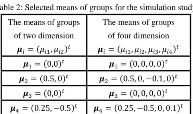
𝐲𝑖𝑗 ~ 𝑁𝑝(𝜇𝑖, ∑) under an alternative hypothesis 𝐻1∶ 𝝁𝑖≠ 𝝁𝑗 𝑓𝑜𝑟 𝑎𝑡 𝑙𝑎𝑒𝑠𝑡 𝑜𝑛𝑒 𝑜𝑓 𝑖 ≠ 𝑗 . The same combinations of dimensions 𝑝, number of groups 𝑘, sample sizes 𝑛𝑖 , 𝑖 = 1, 2, ⋯ , 𝑘 and correlation coefficients 𝜌 as in the experiments for studying the significance level will be used but each group has a different mean 𝝁𝑖= (𝜇𝑖1, 𝜇𝑖2, ⋯ , 𝜇𝑖𝑝)𝑡. The means of dimensions 𝑝 = {2,4} for the groups 𝑖 = 1, 2, 3, 4 are selected as shown in the table 2.

Again, the classical statistic and the robust statistic are calculated. This is repeated 𝑅 = 1000 times and then calculate the power of test 𝜋̂ = 𝐾(𝑇)/𝑅 (where 𝐾(𝑇) is the number of times of rejected the test statistic when the hypothesis is false) of the test statistics above.

The results for three and four groups are shown in figures (3) and (4). It is clearly seen that the power of test

𝜋̂ of the robust Wilks' statistic and the classical Wilks' statistic are closely for all investigated combinations of number of groups 𝑘, dimension of observation 𝑝, and group sizes.

4.3 Robustness Comparisons

Now we will investigate the robustness of the one-way MANOVA hypothesis test based on the proposed robust of the Wilks' statistic. For this purpose we will generate data sets under the null hypothesis 𝐻0: 𝝁1=

𝝁2= ⋯ = 𝝁𝑘 and will contaminate them by adding outliers. More precisely the data will be generated from the following contamination model:

𝐲𝑖𝑗~ (1 − 𝜀)𝑁𝑝(𝟎, ∑) + 𝜀 𝑁𝑝(𝝁𝑖, 0.1∑) where 𝝁𝑖= (5 + 𝑝, 5 + 𝑝, ⋯ , 5 + 𝑝)𝑡, ∑ = (1 − 𝜌)𝐼 + 𝜌𝐽 and 𝜀 = 0.1

The same combinations of dimensions 𝑝, numbers of groups 𝑘, sample sizes 𝑛𝑖 , 𝑖 = 1,2, ⋯ , 𝑘 and correlation coefficients 𝜌 as in the experiments for studying the significance level will be used.

The results of the type I error rates 𝛼̂ and the power of test 𝜋̂ of our statistics for three and four groups are shown in figures (5) - (8). In figures (5) and (6) the type I error rates for the classical Wilks' statistic lie outside of the standard deviation interval (0.036, 0.064). Hence, the classical Wilks' statistic is very bad compared to the robust Wilks' statistic for all the different combinations of number of groups 𝑘, dimension of observation 𝑝, and sample sizes.

The figures (7) and (8) show the results of the power of test 𝜋̂ of the robust Wilks' statistic and the classical Wilks' statistic. It is clearly seen that the robust Wilks' statistic is the best compared to the classical Wilks' statistic for all investigated combinations of number of groups 𝑘, dimension of observation 𝑝, and sample sizes.

5 Conclusions

In the present study, the significance level and the power of test were compared with the classical and the robust Wilks' statistic based on RMCD estimator. Various different situations were investigated by changing the dimension, the group sizes, the number of groups, and the correlation coefficient. The results show that, the robust Wilks' statistic based on RMCD estimator is closely to the classical Wilks' statistic in case of normal distribution for the data set, while in case of contaminated distribution the method in question is robust and efficient comparison with the classical Wilks' statistic which is very bad.

(6)

References

Ameen, A. A. (2007),"Robust Hotelling 𝑇2_{, Wilks'}_Λ_and_𝑅2_{Statistics to Test A Hypothesis for Equality of} Two Multivariate Means and Testing The Contribution of Individual Variables on These Statistics", Ph.D. Thesis, College of Sciences, University of Basra.

Anderson, T. (1958), "An Introduction to Multivariate Statistical Analysis", John Wiley and Sons, New York. Beak, R. C. and Cook, R. D. (1983), "Outliers", Technometrics, Vol.25, 119-149.

Campbell, N. A. (1980), "Robust Procedures in Multivariate Analysis I: Robust Covariance Estimation", Applied Statistics, 29(3), 231-239.

Croux, C., Haesbroeck, G. and Rousseeuw, P. J. (2002)," Location Adjustment for the Minimum Volume Ellipsoid Estimator", Statistics and Computing 12: 191–200.

Rencher, A. C. (2002), "Methods of Multivariate Analysis", Second Edition, John Wiley and Sons, New York. Rousseeuw, P.J., (1985), "Multivariate estimation with high breakdown point". In: Grossman, W., P5ug, G., Vincze, I., Wertz, W. (Eds.), Mathematical Statistics and Applications, Vol. B. Reidel, Dordrecht, pp. 283–297. Rousseeuw P. J., and Van Driessen, K. (1999), "A fast algorithm for the minimum covariance determinant estimator", Technometrics, 41(3), 212-223.

Meral Candan and Serpil Aktas (2003), "Hotelling's Statistic Based on Minimum Volume Ellipsoid Estimator", G. U. Journal of Science, 16(4), 691-695.

Salter, K.C. and Fawcett, R.F. (1989), "A robust and powerful rank test of treatment effects in balanced incomplete block designs", Communications in Partial Differential Equations, 14(4), 807-828.

Todorov, V. and Filzmoser, P. (2010), "Robust Statistic for the One-Way MANOVA", Computational Statistics and Data Analysis, 54, 37-48.

Van Aelst, S. and Willems, G. (2011), "Robust and Efficient One-Way MANOVA Tests", Journal of the American Statistical Association, 106-494.

Willems, G., Pison, G., Rousseeuw, P. J. and Van Aelst, S. (2002),"A robust Hotelling Test", Metrika, 55,125-138.

Table 1: Selected group sizes for the simulation study Three groups (𝑛1, 𝑛2, 𝑛3) Four groups (𝑛1, 𝑛2, 𝑛3, 𝑛4) (10, 10,10) (10, 10, 10, 10) (10, 20, 20) (10, 20,20, 30) (30, 30, 30) (30,30, 30, 30)

Table 2: Selected means of groups for the simulation study The means of groups

of two dimension

𝝁𝑖= (𝜇𝑖1, 𝜇𝑖2)𝑡

The means of groups of four dimension 𝝁𝑖= (𝜇𝑖1, 𝜇𝑖2, 𝜇𝑖3, 𝜇𝑖4)𝑡 𝝁1= (0,0)𝑡 𝝁1= (0, 0, 0, 0)𝑡 𝝁2= (0.5, 0)𝑡 𝝁2= (0.5, 0, −0.1, 0)𝑡 𝝁3= (0,0)𝑡 𝝁3= (0, 0, 0, 0)𝑡 𝝁4= (0.25, −0.5)𝑡 𝝁4= (0.25, −0.5, 0, 0.1)𝑡

(7)

Figure (1)

The type I error plots for the classical and robust Wilks' statistics when the data are followed multivariate normal distribution with 𝑘 = 3, the left side is for 𝑝 = 2, and the right side is for 𝑝 = 4, with three cases of sample sizes where the top part is for 𝑛1= 10, 𝑛2= 10, 𝑛3= 10, the middle part is for 𝑛1= 10, 𝑛2= 20, 𝑛3= 20, and the bottom part is for 𝑛1= 30, 𝑛2= 30, 𝑛3= 30.

0 0.1 0.2 0.3 0.4 0.5 0.6 0.7 0.8 0.9 0.02 0.03 0.04 0.05 0.06 0.07 0.08 0.037 0.063 Correlation Coefficient S ig ni fica nce L eve l Classic Wilks

Robust Wilks based on RMCD

(8)

Figure (2)

The type I error plots for the classical and robust Wilks' statistics when the data are followed multivariate normal distribution with 𝑘 = 4, the left side is for 𝑝 = 2, and the right side is for 𝑝 = 4, with three cases of sample sizes where the top part is for 𝑛1= 10, 𝑛2= 10, 𝑛3= 10, 𝑛4= 10, the middle part is for 𝑛1= 10, 𝑛2=

20, 𝑛3= 20, 𝑛4= 30, and the bottom part is for 𝑛1= 30, 𝑛2= 30, 𝑛3= 30, 𝑛4= 30.

(9)

Figure (3)

The power of test plots for the classical and robust Wilks' statistics for the data from multivariate normal distribution with 𝑘 = 3, the left side for 𝑝 = 2, and the right side is for 𝑝 = 4, with three cases of sample sizes, the top part 𝑛1= 10, 𝑛2= 10, 𝑛3= 10, the middle part 𝑛1= 10, 𝑛2= 20, 𝑛3= 20, and the bottom part

𝑛1= 30, 𝑛2= 30, 𝑛3= 30. 0 0.1 0.2 0.3 0.4 0.5 0.6 0.7 0.8 0.9 0 0.1 0.2 0.3 0.4 0.5 0.6 0.7 0.8 0.9 1 Correlation Coefficient P ow er o f t est Classic Wilks

0 0.1 0.2 0.3 0.4 0.5 0.6 0.7 0.8 0.9 0 0.1 0.2 0.3 0.4 0.5 0.6 0.7 0.8 0.9 1 Correlation Coefficient P ow er o f t est Classic Wilks

(10)

Figure (4)

The power of test plots for the classical and robust Wilks' statistic for the data from multivariate normal distribution with 𝑘 = 4, the left side for 𝑝 = 2, and the right side is for 𝑝 = 4, with three cases of sample sizes, the top part 𝑛1= 10, 𝑛2= 10, 𝑛3= 10, the middle part 𝑛1= 10, 𝑛2= 20, 𝑛3= 20, and the bottom part

(11)

Figure (5)

The type I error plots for the classical and robust Wilks' statistic for the data from multivariate contaminated distribution with 𝑘 = 3, the left side for 𝑝 = 2, and the right side is for 𝑝 = 4, with three cases of sample sizes, the top part 𝑛1= 10, 𝑛2= 10, 𝑛3= 10, the middle part 𝑛1= 10, 𝑛2= 20, 𝑛3= 20, and the bottom part

𝑛1= 30, 𝑛2= 30, 𝑛3= 30. 0 0.1 0.2 0.3 0.4 0.5 0.6 0.7 0.8 0.9 0 0.01 0.02 0.03 0.04 0.05 0.06 0.07 0.08 0.037 0.063 Correlation Coefficient S ig ni fica nce L eve l Classic Wilks

0 0.1 0.2 0.3 0.4 0.5 0.6 0.7 0.8 0.9 0 0.01 0.02 0.03 0.04 0.05 0.06 0.07 0.08 0.037 0.063 Correlation Coefficient S ig ni fica nce L eve l Classic Wilks

(12)

Figure (6)

The type I error plots for the classical and robust Wilks' statistics for the data from multivariate contaminated distribution with 𝑘 = 4, the left side for 𝑝 = 2, and the right side is for 𝑝 = 4, with three cases of sample sizes, the top part 𝑛1= 10, 𝑛2= 10, 𝑛3= 10, 𝑛4= 10, the middle part 𝑛1= 10, 𝑛2= 20, 𝑛3= 20, 𝑛4= 30, and the bottom part 𝑛1= 30, 𝑛2= 30, 𝑛3= 30, 𝑛4= 30. 0 0.1 0.2 0.3 0.4 0.5 0.6 0.7 0.8 0.9 0 0.01 0.02 0.03 0.04 0.05 0.06 0.07 0.08 0.037 0.063 Correlation Coefficient S ig ni fica nce L eve l Classic Wilks

(13)

Figure (7)

The power of test plots for the classical and robust Wilks' statistics for the data from multivariate contaminated distribution with 𝑘 = 3, the left side for 𝑝 = 2, and the right side is for 𝑝 = 4, with three cases of sample sizes, the top part 𝑛1= 10, 𝑛2= 10, 𝑛3= 10, the middle part 𝑛1= 10, 𝑛2= 20, 𝑛3= 20, and the bottom part

(14)

Figure (8)

The power of test plots for the classical and robust Wilks' statistics for the data from multivariate contaminated distribution with 𝑘 = 4, the left side for 𝑝 = 2, and the right side is for 𝑝 = 4, with three cases of sample sizes, the top part 𝑛1= 10, 𝑛2= 10, 𝑛3= 10, 𝑛4= 10, the middle part 𝑛1= 10, 𝑛2= 20, 𝑛3= 20, 𝑛4= 30, and the bottom part 𝑛1= 30, 𝑛2= 30, 𝑛3= 30, 𝑛4= 30. 0 0.1 0.2 0.3 0.4 0.5 0.6 0.7 0.8 0.9 0 0.1 0.2 0.3 0.4 0.5 0.6 0.7 0.8 0.9 1 Correlation Coefficient P ow er o f t est Classic Wilks