Extending Hyperband with Model-Based Sampling Strategies

(1)

Ludwig-Maximilians-Universität München

Faculty for Mathematics, Computer Science and Statistics

Master Thesis

Extending Hyperband with Model-Based Sampling Strategies

Author:

Niklas

Klein

Supervisors:

Prof. Dr. Bernd

Bischl

Janek

Thomas

(2)

(3)

Declaration

I hereby confirm that I have written the accompanying thesis by myself, without contributions from any sources other than those cited in the text and bibliography.

Munich, May 7, 2018

(4)

Abstract

We address the problem of hyperparameter optimization for machine learning algorithms. This is a difficult task for two main reasons: On one hand, the function modelled by the machine learning algorithm is usually derivative free (black-box). On the other hand, function evaluations are typically very expensive in terms of their computational time.

The focus of this thesis lies mainly on the hyperparameters of gradient boosting models and neural networks. Both methods contain a large amount of interdependent hyperparameters. This makes the optimization especially difficult.

Simple optimization approaches such as grid or random search generally do not provide satisfying results. We are going to examine more sophisticated strategies like Bayesian Optimization which try to model the underlying black-box function in order to find a better configuration.

A more recent approach is given by Hyperband, which is the eponym of this thesis. In essence, it adaptively allocates resources across a set of randomly sampled configurations based on their performances. We will explore this algorithm in detail and eventually propose a possible way of combining the advantages of model-based optimization and Hyperband. Afterwards, we present our implementation of Hyperband which we based on the R6 class system. This object oriented variant provides a very generic framework which enables the user to easily modify the conventional Hyperband algorithm. We finally present the results of a benchmark experiment where we compare the aforementioned combination of Hyperband and MBO with the original algorithm. Our findings show that for boosting models, both variants perform about equal (for few training iterations, the hybrid optimizer outperforms the conventional Hyperband while for more training iterations, it is the other way around). When considering neural networks, for which Hyperband was initially intended, both Hyperband-based methods outshine the base line model (e.g. a Random Search). Particularly striking is the fact that even though our hybrid approach generated an overhead (through the additional computations resulting from the model-based procedure), it generally needed less computational time than the conventional Hyperband.

(5)

(6)

1 Introduction

Boosting algorithms and neural networks tend to be very complex systems. Many small ingredients interact in a very elusive manner. In addition to this, particularly the neural networks architectures have become much more complicated. For both methods we address the problem of finding a good set of hyperparameters. These cover the actual settings of our algorithm and must be declared outside of the training phase. Hence, we do not directly target the model parameters. The latter ones are optimized during the training phase (e.g. the weights of a convolutional neural network).

One scope of hyperparameters is to control the flexibility of the model. Figure 1 shows the training progress of an arbitrary neural network. After roughly 10−15 training iterations, the validation loss (turquoise) begins to increase. It is arguable that the model begins to adapt to the training data too much. But hyperparameters may include many other components, depending on the algorithm at hand.

Figure 1: An arbitrary neural network. On the x-axis we see the epochs. That is one forward and one backward pass across the whole training set. By contrast, the y-axis shows the loss of the network. The red curve represents the training and the turquoise one the validation error. After roughly 15 epochs of training, the net seems to begin overfitting the training data.

Machine learning algorithms in general are sometimes referred to as “black boxes”. In science, a black box is a system where one has no knowledge of its internal mechanics (see Figure 2). This could be a computer program, where the user is not allowed to see the code (e.g. due to a closed source program). But also the human brain is considered to be a black box.

So when people use this metaphor for machine learning algorithms, they actually try to paraphrase the vast difficulty of tuning these machines. Severe trouble is mainly caused by the interaction of each of its components and the very costly evaluations. Hence, machine learning algorithms are no black boxes as such. To clarify the reasoning, consider the following thought experiment from Card (2017):

(10)

We have some switches and buttons, which represent our hyperparameters. By modifying their state we cause light bulbs to either power or remain disabled. For a small system we could learn the mechanics of our black box by trying all possible input combinations. Unfortunately, as the system grows in size this approach becomes more and more difficult, if not impossible. Even if we obtain access to the wiring diagram, which is our black box, we will not be able to fully explain its behaviour. This is due to the fact that complexity originates primarily from the interaction of ordinary components.

In the context of machine learning, our algorithms are very complicated wiring diagrams which we have access to, and the buttons are the corresponding hyperparameters. Testing a new input combination is usually very expensive in terms of a given budget (e.g. the time).

Figure 2: A black box uses inputs to generate outputs. For the observer it is not possible to comprehend the procedures inside of the black box. He may only see the input and the corresponding output.

(11)

2 The Hyperparameter Optimization Problem

In this chapter we introduce both, gradient boosting and neural networks.

After a short introduction to each methods mechanics, we aim towards their individual hyperpa-rameters and the arising difficulties to find a good composition of them.

2.1 Gradient Boosting

In the world of supervised learning, we usually have a vector of input variables xand an output variabley. The goal is to use a labeled training set {(x(1), y(1)), . . . ,(x(n), y(n))} to approximate a functionf, which minimizes the empirical risk Remp =Pni=1L(y(i), f(x(i))): ,

ˆ

f = arg min

f

Remp (1)

Gradient boosting (Friedman 2001) is an ensemble method and very successful at this task. 2.1.1 Brief Introduction

We can think of a gradient boosting model as the weighted sum of many weak learners b:

ˆ f(x) = M X m=1 ˆ β[m]b(x,θˆ[m]) (2) These weak learners, solely, are relatively poor performing predictors and in general just slightly above chance. A common choice are small trees or even stumps. So when composing a new boosting model, we gradually add these weak learners to our ensemble. For each weak learner we impose the requirement to improve the overall performance of our model. This is were the eponym of the model class becomes apparent. At each boosting iteration m and for all observations i, we compute the negative gradient of our loss function L:

r[m](i)=−

_δL(_y(i)_{, f}(_x(i)))

δf(x(i))

(3) The r[m](i) _{are called pseudo residuals and tell us which way to go in function space in order to} reduce the loss. Following up, we fit a weak learner on the negative gradient vector r[m]_:

ˆ θ[m]= arg min θ n X n=1 (r[m](i)−b(x(i), θ))2 (4) We can think of this concept as fitting a weak learner on the error of the current model. Up next, we find our weighting parameter ˆβ by conducting a line search. To finish the boosting iteration, we add both parts into our ensemble:

(12)

ˆ

f[m](x) = ˆf[m−1](x) + ˆβ[m]b(x,θˆ[m])) (5) In the next iteration, we simply repeat the process by fitting another weak learner on the error of the updated model. This approach is also called forward stagewise additive modelling. An advantageous aspect of gradient boosting is that it generalizes the idea of boosting. This means that we are allowed to use an arbitrary loss function. Hence, in order to conduct classification, all we have to do is to select it appropriately (e.g. the binomial loss for binary classification problems).

2.1.2 XGBoost and its Hyperparameters

One of the most famous boosting frameworks is XGBoost, an abbreviation for extreme gradient boosting (Chen et al. 2018). It provides a highly parallelized tree boosting implementation and contributed to many winning solutions in various Kaggle challenges. An essential characteristic is its huge variety of regularization parameters. For instance, consider its risk function:

R[m] emp= n X i=1 L(y(i), f[m−1](x(i)) +b[m](x(i))) +γJ1(b[m]) +λJ2(b[m]) +αJ3(b[m]) | {z } regularization (6) The leading part is essentially the same as we introduced in section 2.1. But behind that we observe three additional terms. The first component γ covers the minimum loss reduction required to make a further split (we can think of the tree depth). Additionally, λ introduces an L2 and α an L1 regularization on the models weights.

But these are by no means all hyperparameters we have to deal with. We have to incorporate a learning rateν, shrinking the step size of each iteration:

ˆ

f[m](x) = ˆf[m−1](x) +νβˆ[m]b(x,θˆ[m])) (7) This can also be regarded as a regularization in order to prevent overfitting. While γ affects the tree size indirectly, we can also opt to cap it in a rule-based fashion (e.g. a maximum tree depth). The subsample parameter defines the fraction of observations to be randomly sampled for each tree. Inspired by random forests, another regularization technique is feature subsampling (Chen & Guestrin 2016). We can choose to incorporate only a certain subset of columns when growing a tree. Going one step further, we are even able to subsample the features at each split in our trees. Table 1 summarizes the introduced parameter set.

It becomes immediately apparent that finding the right configuration is very hard. Chapter 3 will introduce various techniques to tackle this issue.

(13)

Table 1: XGBoost feasible hyperparameters. Most of them aim towards regularization. The range column indicates each hyperparameters possible region for their values.

parameter range description

γ [0,∞] minimum loss reduction required to make a split λ L2 regularization term on the weights α L1 regularization term on the weights max_depth The maximum allowed depth of each tree

subsample (0,1] fraction of randomly sampled instances for each tree colsample_bytree (0,1] fraction of randomly sampled features for each tree colsample_bylevel (0,1] fraction of randomly sampled features for each split

(14)

2.2 Neural Networks

As of 2018, neural networks play a vital role in many fields. For sophisticated projects, such as the realization of autonomous cars, they can act in a supportive fashion. This includes subtasks for the perception and localization of the car as well as the control over the drivers state (Fridman 2018). Neural networks also find use for mundane tasks, like speech recognition. In order to predict the input sequence of phonetic states from audio data, Amazons virtual assistant “Alexa” utilizes a distributed variant of recurrent neural networks (Strom 2015). But also expert problems, like the analysis of medical images, are being tackled successfully by deep neural networks (Qayyum et al. 2017).

2.2.1 Introduction

Neural networks in general integrate the process of feature engineering into their modeling pipeline. The closer past has shown that this works particularly well for certain types of data. Judging by the results of the annual ImageNet contest (Russakovsky et al. 2015), convolutional neural networks represent the undisputed state of the art for image processing. This covers for instance object and speech recognition, but also segmentation exercises.

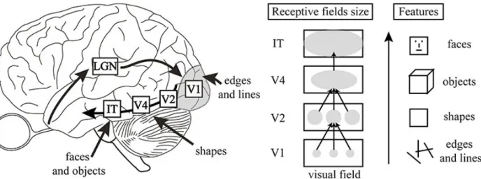
Convolutional neural networks, from now on abbreviated CNNs, are inspired by the visual cortex of mammals. Figure 3 describes the fundamental idea. Initially, a stage named V1 extracts so called low level features. These include edges, lines or color gradients. Subsequent stages assemble these low level features to increasingly compounded structures. We can think of ordinary Lego bricks in the first stage. These are plugged together to form shapes as depicted by stage V2. Finally, these shapes are assembled to yield “complete” objects as depicted by stageV4. Eventually, the human brain can recognize such objects and assign them to a class (e.g. a face).

Figure 3: Visual cortex and feature extraction (Herzog & Clarke 2014). The image describes how the visual cortex of a human works. The assembly of low level features (e.g. edges, lines or color gradients) leads to complex high level features such as faces.

To cast this idea into a model, we have to become acquainted with the name giver of the model class, which is the discrete convolution. Consider Figure 4a. The left side shows a simple

(15)

black-and-white image. In contrast, the right side represents the associated pixel entries (i.e. what a computer “sees”). We deduce zeroes representing the color black, 255 the color white and everything in between the gray levels.

Now suppose we would like to detect vertical edges in that image. One way to achieve this is by applying a filter called Sobel-Operator (Sobel 1968). Figure 4b shows one step of the required procedure. We position the Sobel-Operator on the red framed location of the image and compute the dot product. That is:

S(i,j)= (I ?Gx)(i,j)=−1·0 + 0·255 + 1·255

−2·0 + 0·0 + 2·255 (8)

−1·0 + 0·255 + 1·255

where Si,j indicates the output at row iand column j. The ? implies convolution between the

input image I and the filter Gx. After applying the filter to every feasible location of our input

image (Figure 4c), we have to normalize the pixel entries, as can be seen in Figure 4d. The resulting output array is called feature map.

What the Sobel-Operator actually did was investigating the neighborhood of each central pixel. Technically, this equals the computation of an approximation of the gradient.

(a) How to represent a digital image: ordinary black-and-white image on the left, pixel entries on the right. Zeros indicate the color black, 255 the color white and everything in in between the gray levels.

(b) Exemplary application of the Sobel-Operator on an arbitrary location of our input image. We simply compute the dot product to obtain the convolved value: Si,j = 1·255 + 2·255 + 1·255 = 1020 (more details of the computation can be seen in Equation 8).

(16)

(c) Results after applying the Sobel-Operator to every possible location in our input image. Framed in red: the outcome of the application of the Sobel-Operator to the area shown in Figure 4b.

(d)Normalized pixel values to reveal the vertical edges in the input image. The corresponding image is called feature map.

Figure 4: Applying the Sobel-Operator on a black-and-white image in order to detect vertical edges.

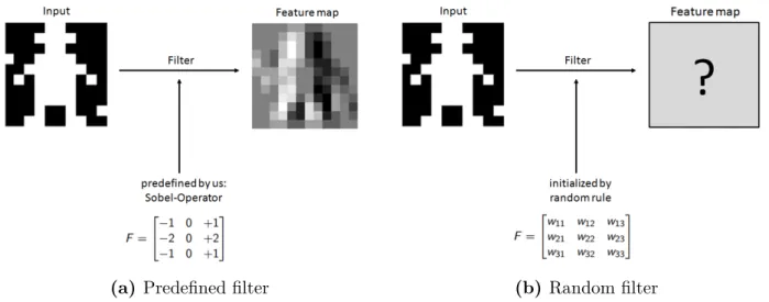
Figure 5a summarizes what happened: a predefined filter was used to convolve the input image into a feature map. What a convolutional neural network does is very similar. One crucial difference arises in the fashion filter entries, which are our model parameters, are selected. In fact, a CNN initializes them by a random rule (see Figure 5b).

(a) Predefined filter (b) Random filter

(17)

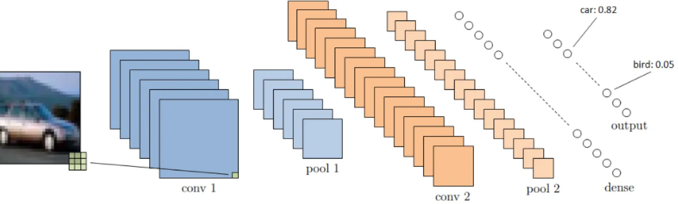
To construct a model of this idea, we use filters for automatic feature extraction and dense layers to associate them. Suppose we would like to recognize objects from the CIFAR-10 dataset (Krizhevsky 2009). It consists of 60.000 32×32 color images, evenly distributed over 10 classes. Those classes are cars, trucks, airplanes, birds and other animals. A potential architecture to do this could look like it is shown in Figure 6. We have some feature maps in our first layer. Each of them is constructed by an individual, randomly initialized filter.

Figure 6: Architecture of a small convolutional neural network. The model has two convolution and corre-sponding pooling layers, followed by one dense and one output layer.

Subsequently we apply an operation called pooling to reduce the size of our feature maps. As a consequence, we get rid of a lot of data. One advantage is that our computation is less expensive. While doing so, we try to retain as much information as possible. One typical approach for this is called max pooling and depicted by Figure 7. We use the common filter size 2 as well as the standard step size of 2. That means that for each 2×2 block we extract its maximum value and eventually quarter the size of our feature map.

Our model architecture of Figure 6 repeats the whole procedure one more time. In the second round we use the features of pooling layer 1 to produce the second convolution layer. That is the part where we plug our Lego bricks together in order to build more sophisticated structures.

Figure 7: Max pooling procedure. The blue array represents a feature map. We choose a 2×2 filter and a step size of 2. For each 2×2 block, we extract the maximum value. At the first location we obtainmax{2,8,4,3}= 8. The two by two rectangle represents the pooled feature map.

Finally, we feed the features which are contained in pooling layer 2 into a dense layer. This is our actual predictor. Each time we propagate a batch of images through the network, we compare the results of our predictor with the ground truth. For each of our parameters and quite similar to chapter 2.1.1, we compute the negative gradient of a loss function. This will tell us in which way we have to adjust each parameter of our model, in order to reduce the

(18)

loss. We call this propagating the error backwards through the net to measure each parameter’s contribution to it. To obtain a good model, we have to repeat this step many times. Thus, fitting a neural networks is an iterative procedure. One forward pass and one backward pass across the whole training set is called epoch. Generally, we repeat the whole technique for multiple epochs.

2.2.2 Hyperparameters of a Neural Network

When we decide to address a problem with a neural network, the first challenge is to find a suitable architecture. Once we found a basic framework to operate with, the next problem appears:

Neural networks have an inconceivable amount of hyperparameters, which makes tuning very hard. In order to ease the problem a little bit we settle on the architecture of Figure 6. That means that we fixate some hyperparameters, such as filter sizes or the amount of feature maps and neurons in all layers.

A feasible architecture is demonstrated by Table 2. Since CIFAR-10 contains only color images, we have to incorporate three channels (red, green and blue) for the filters of our first conv layer. As a consequence, each filter in layer one has 3×3×3 = 27 parameters. Including the bias, the first layer has a total of 33_×_{8 + 8 = 224 model parameters. The whole architecture has 66}_._634, while most of them result from the dense layer with 64 neurons (1.024×64 + 64 = 65.600) Table 2: Model architecture of Figure 6. Since we’re dealing with color images, the filter of our first layer has to incorporate the channels of the RGB color model. Hence, each 3×3 filter of layer one has 33_{= 27 parameters.} For convolution filters we chose padding and a step size of 1. Thus, both conv layers will conserve its inputs height and width. The pooling filters have a dimension of 2×2 as well as a step size of 2.

layer filter/neurons feature maps model parameters current dimension

conv 1 3×3×3 8 224 32×32 pool 1 2×2 16×16 conv 2 3×3 16 160 16×16 pool 2 2×2 8×8 flatten 1×1.024 dense 120 65.600 output 10 1.210 total 66.634

Before we can utilize this architecture, some obligatory hyperparameters must be set.

(19)

of each weight. This is done by an enveloping optimization algorithm. Figure 8 shows that beside stochastic gradient descent, a lot more options to choose from are available. While the three shown examples all share the “sub-hyperparameters” learning rate and learning rate decay, they also introduce some individual ones. For example, when we opt for sgd, we also have to find a good value for momentum and decide whether we want to apply nesterov or not.

Figure 8: The optimizers for a neural network. All shown examples share some “sub-hyperparameters”. For instance the learning rate or the learning rate decay. But they also introduce individual ones, which makes the search for the right choice even more difficult.

Another global hyperparameter is the batch size. If we set it too small, convergence will take really long. Choosing it to high, the performance of our model will very likely suffer (Keskar et al. 2016). There is also a strong interaction between the learning rate and the batch size. A larger batch size requires a smaller learning rate. Smith et al. (2017) propose adaptive batch sizes. They argue that after some epochs with small batches, we have very likely skipped bad local minima and eventually converge into a good point faster.

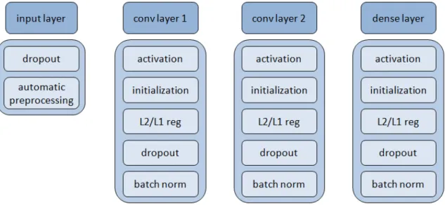
Figure 9: Layers and hyperparameters. Particularly appealing when dealing with image data, one could utilize dataset augmentation on the input as automatic preprocessing. For conv and dense layers, a crucial hyperparameter is the activation function. Furthermore, a wide range of regularization parameters are available.

(20)

Each individual layer represents another building block full of hyperparameters. That includes the input as well. We could opt to apply live dataset augmentation within our model pipeline. For images one can think of flipping each instance by a given degree as well as mirroring each of them. Doing that, we can easily increase our train set by a magnitude of 8.

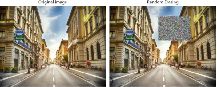
Zhong et al. (2017) even apply regularization on the input by randomly erasing parts of each image (see Figure 10).

Figure 10: Randomly erasing parts of input images in order to increase regularization (Zhong et al. 2017).

As we progress to the actual layers, one indispensable hyperparameter is a set of activation functions. They are attached at the end of each layer and supply the model with non-linearity. While the standard ReLU (max(0, x)) is usually a good choice, more sophisticated mutations are operational. For instance the LeakyReLU, which aims to fix the dying ReLU problem. The latter one means that a ReLU outputs 0 for any input and since the gradient at that state is also always 0, it is very unlikely that it can recover on its own. LeakyReLUs try to overcome this issue by assigning a very small negative slope for values x <0 (Maas et al. 2013).

When we start the training process, we initialize all model parameters by a certain rule. This weight initialization can have a significant impact on the networks convergence rate and thus on the overall quality of a model. The neural network library Keras (Chollet 2015) for example provides over 15 variants. Those include conventional sampling from a normal distribution but also advanced techniques that incorporate the structure of the input data. Xavier initialization for instance tries to match the variance of the outputs of a layer with the variance of its inputs. According to their inventors, this is working particularly well for layers with sigmoidal activation functions (Glorot & Bengio 2010). He et al. (2015) captured this idea and customized a version called “He normal” for the ReLU family.

Each layer of a neural network can be furnished with various regularization techniques. One of the most famous is called Dropout (Srivastava et al. 2014). For each batch that we propagate through the network, a preset fraction of neurons will be randomly deactivated. It is believed that this prevents hidden units from learning every detail of the data and thus to memorize it.

(21)

deep learning, the latter one is commonly known as weight decay).

A recent advance in deep learning is called batch normalization (Ioffe & Szegedy 2015). The idea is to normalize the distribution of each input unit of a layer across the current batch. Since the inputs for the next layer are based on all instances of the current batch, it does also introduce regularization, as well as an interaction with the learning rate. Their originators claim that batch normalization enables the usage of higher learner rates which will speed up training time. While we covered a striking amount of hyperparameters, it still represents only a small fraction of possibilities when dealing with neural networks. Many more subject-specific options like gradient clipping or the choice of custom tailored right loss functions can be taken into account.

(22)

3 Methods for Hyperparameter Optimization

The last chapter introduced gradient boosting, and technically speaking, convolutional neural networks. Both methods provide a large variety of hyperparameters. This makes the search for a good composition very tedious. People quite often do not have sufficient experience to “guess” good parameters. They typically rely on default or recommended values. Unfortunately, these are not always suitable for the problem at hand.

This issue is aggravated by the fact that literature on good tuning techniques is very under-represented (Bischl 2017). Brute force methods like grid search are easy to implement but not really helpful. The combinatorial explosion makes it very expensive. In addition to this, it will very likely waste a lot of time on irrelevant areas. Likewise, as it relies purely on luck, random search isn’t a reliable choice either. Yet, it often serves as the standard baseline model.

The upcoming subchapter introduces a much more sophisticated technique which is called Bayesian or model-based optimization. Its central idea is to propose new configurations in a sequential fashion.

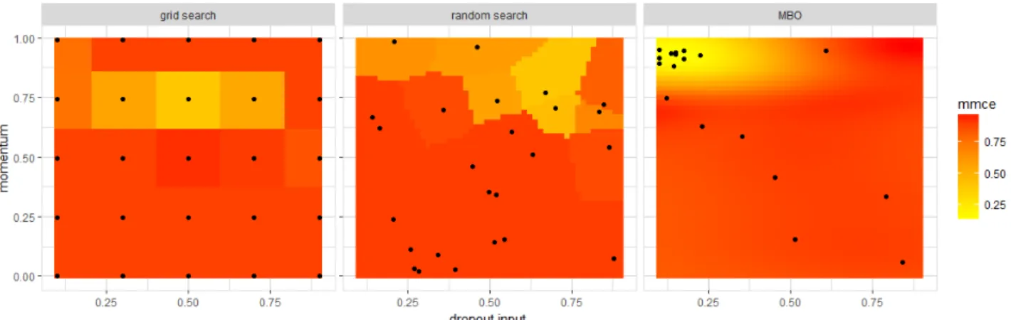
Figure 11 hints at each method’s characteristics. Here we try to find a good combination of momentum and input dropout for a neural network. Suppose we are limited by a temporal restriction and thus can only train for 10 epochs. Obviously, we want a high momentum in combination with a low to medium dropout value. The grid search spends a lot of resources in bad areas. Random search does basically the same. MBO however quickly zeros itself in on a promising area. Both grid search and random search perform 25 model evaluations. Their lowest mean missclassification errors (mmce) are 34.53% and 39.25% respectively. Despite conducting only 18 model evaluations, MBO manages to get a mmce of 11.46%.

Figure 11: Grid search, random search and MBO. We try to find a good combination of momentum and input dropout. Both grid search and random search waste a lot of resources on irrelevant ares. MBO needs fewer evaluations to find a better configuration. Its lowest mmce is at 11.46%, while random search and grid search only manage to get an error of 34.53% and 39.25% respectively.

Chapter 3.2 presents a completely different approach to hyperparameter optimization, called Hyperband. Especially for neural networks, the relatively new algorithm provides state of the art results. In the end we propose a general strategy to combine both methods: model-based optimization and Hyperband.

(23)

3.1 Bayesian Optimization

Assume we would like to minimize an unknown function f. This means in particular that we are not able to compute derivatives. The only thing we can do is to observe the function’s output y for an arbitrary set of input parameters x∈X:

y=f(x) f :_X→_R

To minimize the function, our task is to find the best input combination: x∗ = arg min

x∈_X

f(x)

Now suppose the function is very expensive to evaluate. We can think of a high monetary cost for each trial of an engineering problem. Another paradigm could be a long-term study in order to test the effect a new drug. For machine learning models, the costliness arises from the time it will take to train one model. Therefore, we cannot simply “brute force” a good result by performing an endless amount of evaluations.

Bayesian optimization is a sequential and derivative free approach to tackle these kinds of problems. The central idea is to use regression to approximate the unknown target function. Algorithm 1 briefly describes the general strategy.

We begin to draw |ninit| configurations from the parameter space X. Following up, each one of

them is being evaluated: y(d) =_f(_x(d)). The tuples of configuration and corresponding output are called the initial design:

(x(1), y(1)) (x(2), y(2))

...

(x(ninit)_{, y}(ninit))

In the next step, we fit a regression model on this design. We call it the surrogate model and it essentially tries to interpolate the unknown function. This model must also include predictions for the uncertainty at each location.

A so called infill criterion utilizes this information to propose a new interesting configuration. In a nutshell, it governs the trade-off between exploitation and exploration. To put it another way, if we inspect regions with high variance, we conduct exploration. Going into areas with good estimated values on the other hand means exploitation.

The final step is to evaluate the new configuration and add it to the design. We then repeat the procedure until we exhaust a certain amount of budget (e.g. time).

(24)

Algorithm 1 Bayesian optimization pseudo code 1: Input: budget and parameter space _X

2: Sample|ninit|configurations x(d) fromX.

3: Evaluate each configuration: y(d) =f(x(d)) We call the tuples (y(d)_{, x}(d))_,_∀_d_∈(1_{, ..., n}

init) theinitial design.

4: while budget not exhausted do

5: Fit a regression model on the current design to predict ˆf(x). We call this the surrogate model.

6: Propose a new configuration x(d+1) _{via an infill criterion.}

This governs the trade-off between exploitation and exploration. 7: Evaluate the new configuration and add it the the design

8: end while

9: return best configuration

In order to obtain a better understanding of this intuition, let us consider a graphic example. Suppose we would like to find the minimum of Equation 9:

f(x) =x2+sin(1.1·π·x) (9) While in practice this would be unknown, the black solid line in each top plot of Figure 12a, b, c and d shows the functions true course.

We choose ninit = 3 for our initial design. The evaluated configurations are represented by the

three red points in Figure 12a. Based on them, the dashed line in the upper plot of Figure 12a represents the current prediction of the surrogate model.

Highlighted in grey we also see the prediction of the standard error. These are the areas we mean when speaking of exploration. The bottom plot of Figure 12a show the infill criterion (here we use the expected improvement “ei”, which will be discussed in more detail in section 3.1.3). Its maximum value tells us which configuration we should try next (the blue triangle in the upper plot).

Figure 12b shows the updated surrogate model. A green square depicts the new configuration which is now also part of our design. In this iteration, the infill criterion leads us almost to the global optimum of the function.

The third iteration is portrayed by Figure 12c. We can see that the infill criterion now proposes a point which is slightly worse than the previous evaluation.

Figure 12d demonstrates the situation after a total of 5 iterations. Eventually, we end up very close or even at the global minimum.

(25)

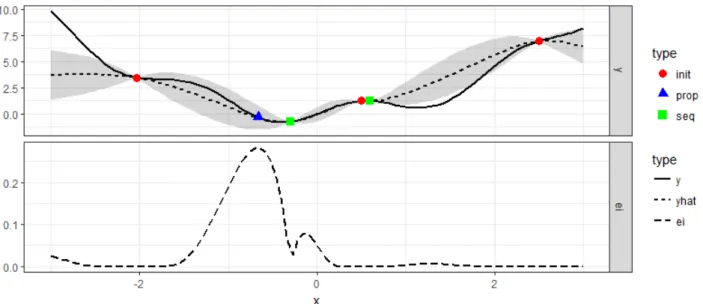
(a) The black solid line in the top plot shows the function of Equation 9 (which we normally know nothing about). Three red dots represent the initial design. A dashed line displays the current prediction of our surrogate model. Shaded in grey we see the standard deviation for each point, which was also estimated by the surrogate model. In the bottom plot, another dashed line represents the infill criterion (here we use the expected improvement, “ei”). It proposes to evaluate the x-value of its maximum next. This configuration is indicated by the blue triangle in the upper plot. Therefore, we decide to exploit instead of explore.

(b) After the first iteration, we incorporate the new point (the green square) into our design. The dashed line in the upper plot shows the new prediction of the surrogate model. According to the infill criterion, we should now evaluate the blue triangle.

(26)

(c) After the second iteration, the infill criterion proposes a new configuration, which is slightly worse than the previous one.

(d) The fifth iteration shows that we end up very close to the global minimum.

Figure 12: Bayesian optimization of Equation 9. We see the development of the surrogate model (black solid line) over 5 iterations. Eventually, we find the global optimum. Both, the computations and plots were realized with the mlrMBO package (Bischl et al. 2017).

3.1.1 Initial Design

The first step in Bayesian optimization entails the creation of an initial design. This initial design represents the foundation for our surrogate model. Two common alternatives to obtain a set of configurations include random and latin hypercube sampling (LHS).

LHS will maximize the minimum distance between the configurations. Figure 13 shows a simple example for a problem with two parameters. In Figure 13b we can see that random sampling may result in very akin configurations. Yet in certain situations, unequal distances might even be advantageous (Morar et al. 2017).

(27)

(a) Sampling with LHS (b) Sampling completely at random

Figure 13: LHS vs random sampling. LHS will maximize the minimum distance between each configuration. This ensures more exploration but does not necessarily lead to a better result.

3.1.2 Surrogate Models

The key task of the surrogate model is to interpolate the unknown function f(x). Choosing a model depends mainly on the domain of the input variables. A Gaussian process for instance can only handle numeric values. If we incorporate categorical variables, one possible solution could be supplied by random forests. Both of these methods provide a native uncertainty estimation. This is crucial if we want to use an infill criterion.

Gaussian process

In general, a Gaussian process (GP) is a collection of random variables. Every finite subset of these random variables has a multivariate normal distribution (Snoek et al. 2012). We introduce the GP as the distribution over functions:

f ∼GP(m, K) (10)

where m:_X→_R represents the mean function:

m(x) = E[f(x)] (11)

and K :_X2 _→

R the covariance function:

K(x, x0) =E[(f(x)−m(x))(f(x0)−m(x0))] (12) Now assume we would like to know the function values f(x) for some data points x = (x(1)_{, ..., x}(n)_{). Since} _f₍_x_{) = (}_f₍_x(1)_{, ..., f}₍_x(n)_{)) is a subset of random variables, it has the}

joint distribution

(28)

So basically the entire Gaussian process is defined by its mean and covariance function. In order to infer a new point, we condition the unknown function value on the known ones:

P(f(x(n+1))|x(n+1), f(x(1)), x(1), ..., f(x(n)), x(n))

For each new point the GP returns the mean and the variance of a normal distribution over all possible values of f at x. If there are no “nearby” known points, the mean function will dominate the result. Crucial for this is the choice of the covariance function as it essentially acts as a kernel to measure the similarity of two points.

Recall the problem of Equation 9 and the initial design shown in the upper plot of Figure 12a. Figure 14 compares the standard Gaussian covariance function:

k(h) =exp− 1 2θ2||h|| 2 =exp− 1 2θ2||x, x 0_||2

with the Matérn3/2 (which was also used for the surrogate model of Figure 12): k(h) = 1 + q 3|h| l exp − q 3|h| l

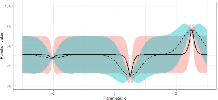
The dashed line represents the Gaussian Kernel and the shaded turquoise area its uncertainty estimation. It appears to be smoother than the Matérn3/2 (the solid black line and the red area respectively). This might be more suitable for problems with little prior knowledge.

Figure 14: Gaussian covariance kernel vs Matérn3/2. The dashed line represents the mean function of the Gaussian kernel. In turquoise, we see its uncertainty estimation. The Matérn3/2 is depicted by the solid line and in red we can see its estimation of the standard error. In the Matérn3/2, the mean function dominates very early. Thus it is a very flexible and general kernel and in addition to that does not assume quite as much smoothness as the Gaussian kernel. Therefore, it might be a good choice when dealing with very little prior knowledge. The plot was generated with the DiceKriging package (Roustant et al. 2012), which uses “kriging”. This is a variant of Gaussian process regression with slightly different assumptions about the mean (Jones et al. 1998).

(29)

Random forests

For mixed parameter spaces which include categorical variables we need another model class. A suitable choice is given by random forests as they naturally handle this kind of data. Random forests are an ensemble learning method, primarily applied on classification and regression problems (Breiman 2001).

To fully understand the idea behind random forests, we have to take a step back and acquaint ourselves with Classification and Regression Trees (Breiman et al. 1984). Such a tree divides the feature space Xinto M rectanglesR and fits a simple model to each of them (e.g. a constant):

f(x) =

M X

m=1

cm1(x∈Rm)

Figure 15 shows the results of three different regression trees. Once again, we use the function of Equation 9 for our demonstration. To compute the model for the left plot, we used 20 equidistant function evaluations (points). The trees of the intermediate and right plot had 30 and 50 observations respectively at their disposal. Several stopping criteria, such as the minimal number of observations per node, prevent the tree from overfitting.

Figure 15: Regression tree on the sinus function of Equation 9. For the left tree we used 20 equidistant function evaluations (points). The tree of the plot in the middle used 30 and the right 50 points respectively. Each classification tree was created with the rpart package (Therneau & Atkinson 2018).

CART is a very simple algorithm. One drawback is its vulnerability to minor changes in the data. If we apply a trained CART model on new data, we will likely experience very high variance. This inevitably means that the predictive performance of a single tree is very poor (Hastie et al. 2009a).

Leo Breiman (1996) proposes bootstrap aggregation (abbreviated bagging) in order to tackle this problem. Bagging means that we create multiple models and average them. The twist is that for each model we draw a small subset of our data D (with replacement). Given this randomization in the training data, we can greatly lower the variance (Hastie et al. 2009a).

ConsiderM identically distributed (but not independent) trees with positive pairwise correlation ρ. We can write the variance of their average as (Hastie et al. 2009b):

ρσ2+ 1−ρ M σ

2 ₍₁₃₎

As we increase the number of treesM, the right term of Equation 13 shrinks away. Unfortunately the correlation part ρσ2 _{still remains. Consequently, at some point we cannot significantly}

(30)

reduce the variance any further by adding more trees into our ensemble.

In order to obtain even lower variance and thus better performance, one has to reduce the correlation between the trees. This effect can be achieved by only picking a random subset of of the p features in the data at each node split:

mtry ≤p

Every single tree is now forced to use different predictors for splitting at every node. Thereby, we now do not only construct bootstrap trees (i.e. trees with different training data), but also more de-correlated ones (Hastie et al. 2009b). Algorithm 2 sums up how the random forest

works. Eventually we obtain an ensemble of trees. For regression, we average the result of all trees.

Algorithm 2 Random Forest

1: Input: Data D, number of trees M, number of variables to draw at each splitmtry 2: for m = 1 to M do

3: Draw a bootstrap sample D[m] _from_D 4: Fit a tree t[m](_x) with data _D[m]

5: For each split consider only mtry randomly selected features 6: Grow tree

7: end for

8: return ensemble of trees: {tm}M

To predict a new point x: Regression: ˆfM₍_x_{) =} 1 M M X m=1 tm(x)

Classification: let ˆCmx be the class prediction of the mth tree.

Then: ˆCM(x) = majority vote{Cˆm(x)}M

To utilize infill criteria, we need an estimation of the uncertainty. Like a Gaussian process, the random forest has this property naturally. In essence it is a consequence of the bagging procedure. We exploit this and compute the mismatch of each single tree’s prediction with the full ensemble: ˆ σ2(x) = 1 M M X m=1 (ˆtm(x)−fˆM(x))2

In this equation ˆtm₍_x_{) corresponds to a tree which was trained with the m’th bagging subset,}

whereas ˆfM₍_x_{) represents the full ensemble.}

3.1.3 Infill Criterions

The infill criterion proposes new configurations. Perhaps the easiest variant is called “mean”. As the name suggests, it does only consider the mean which was estimated by the surrogate model. Figure 16a shows the problem of Equation 9. Our mean infill criterion proposes almost the same location where we already evaluated a configuration. We might even get stuck there.

(31)

(a)

Typically, the infill criterion does also include the uncertainty for its proposal. In other words, it controls the trade-off between exploration and exploitation. One of the most established variants is the expected improvement:

EI(x) =E(I(x)) =E(max{ymin−Y(x),0}) (14)

We can think of this as the search for the greatest potential improvement over the currently best observed value ymin. Y(x) is a random variable representing the posterior distribution at x. In

the case of a Gaussian process surrogate model, the Y(x) corresponds to a normal distribution. Figure 12a, b, c and d used the expected improvement for all of its proposals.

An easier alternative which we need in the last section of this chapter is called lower confidence bound:

LCB(x, λ) = ˆµ(x)−λseˆ(x) (15) The trade-off between the exploitation and exploration is only controlled by a parameter λ. Note that the infill criterion themself requires optimization as well. The mlrMBO package (Bischl et al. 2017) uses a technique called focus search. It basically constructs a huge random design whereof all points are being evaluated by the surrogate model. Following up, the area next to the most promising configuration is shrunken down and the procedure repeated to enforce local convergence.

(32)

3.2 Hyperband

In Bayesian Optimization, we gradually propose new configurations.

Hyperband turns the tables as it instead gradually allocates resources across a set of randomly sampled configurations. For resources, we can think of a budget which is appropriate to the algorithm. In the world of boosting, these resources could be the total number of boosting iterations. A neural network on the other hand has two obvious alternatives: the epochs or the mini batch updates. Also, a temporal resource type would work for both methods.

3.2.1 Successive Halving and the B to n Problem

Li et al. (2016) establish the Hyperband algorithm as a solver for multi-armed bandit problems. In order to understand this, imagine a gambler in a casino who wants to maximize his profit. He is free to choose between n different slot machines and has a fixed budget B. At first glance, he has absolutely no knowledge of each slot machine’s rate of return. So he begins to spend b units of budget for each machine, such that b·n << B. To put it another way, this means “pulling” each bandits armb times. As a consequence, he loses some of his budget B. Likewise, he does also gain a bit of information concerning each machine’s return rates. The upcoming question for the gambler is how to allocate his remaining budget on the bandits.

To translate this idea into our hyperparameter optimization problem, we simply think of configurations instead of armed bandits. This means that a limited amount of resources must be distributed across competing configurations such that we optimize our performance measure. Initially, each configuration’s capabilities are only little known. As we begin to carefully allocate more resources, each configuration might become better understood.

One way to solve the question on how to allocate the resources could be provided by Successive Halving (Jamieson & Talwalkar 2015). Algorithm 3 shows the mechanics.

Summarized, all Successive Halving is doing is to evaluate each configuration and then to eliminate the worse half according to the performance measure. Subsequently, more budget will be allocated to the victors. The whole procedure is repeated for dlog₂ (n)e times, where n represents the total number of initial arms.

Algorithm 3 Successive Halving 1: input: total budget B

2: input: n arms

3: initialize: S0 ← {1,2,3, ..., n} 4: for r = 0 to (dlog₂ (n)e −1)do 5: sample each arm i∈Sr for

br =

B

|Sr|dlog2 (n)e

times, and let ˆpr

i be the reward

6: let Sr+1 be the set of d1₂ ·Sre arms with the largest reward

7: end for

(33)

This, and the budget allocation of line 5 of Algorithm 3, ensure that the entire budget will never be exceeded.

Suppose we had a total budget of B = 1000 and n = 100 arms. Table 3 shows the procedure of the Successive Halving algorithm. At first, we allocate b0 = 1 unit of budget to each of our n = 100 arms. Subsequently, we eliminate the worst 50 arms from our investigation. To each of our remaining arms, we allocate 2 additional resources. Equation 16 shows how to calculate the budget allocation for the second round r = 1. b c represents the floor and d e the ceiling function respectively. br = _B |Sr|dlog2 (n)e = 1000 |S1| |{z} |{1,2,...,50}| dlog₂ (100)e = 2 (16)

After a total of |r|= 7 iterations, we obtain the best arm according to the Successive Halving criterion. Overall, we spent 877 of our 1000 resources.

Table 3: Example for Successive Halving. For a budget ofB= 1000 andn= 100 arms, we conduct a total of |r|= 7 iterations. In the first one, each of our arms receives 1 unit of budget. Next, we filter the worst 50 arms and allocate another 2 units of budget the the victors.

iteration r number of arms left budgetbr for each arm total budget spent

0 100 1 100 1 50 2 200 2 25 5 325 3 13 10 455 4 7 20 595 5 4 35 735 6 2 71 877

Assume we would like to find a good set of hyperparameters for a neural network.

To do this, we are limited by a fixed budget B. In order to conduct Successive Halving, we have to select a number of configurations n which we would like to try. As a consequence, we implicitly decide the amount of resourcesb0 which are allocated to each configuration. Therefore, we also determine how “long” we examine each configuration, until the “bad” ones are being sorted out. For the previous example of Table 3, we obtained b0 = 1.

(34)

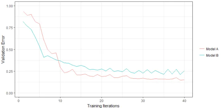
Consider Figure 17. It shows the error-behavior of two arbitrary neural network configurations on the same data. Both curves intersect at roughly 10 training iterations (e.g. epochs). While “Model B” manages to decrease its validation error faster than “Model A”, it does also level off at a higher terminal error. This means in particular, according to the Successive Halving criterion, we would very likely opt for the inferior “Model B”.

To evade the wrong choice in this situation, we required b0 ≥10. For a budget of B = 1000, that only happens if we set n≤20 (see Equation 17).

b0 = 1000 |S0|dlog2 (n)e _! ≥10 (17) ⇔n≤20

This is called the B to n problem. We do not know how to choose n appropriately in order to obtain the best possible configuration. Choosing n too high will very likely lead to wrong decisions. Selecting a value which is too low means that we hardly experience a sufficient range of configurations. Hyperband captures the basic idea of Successive Halving and refines it in order to tackle the B to n problem.

Figure 17: The B ton problem. In red and turquoise, we see the validation loss of two arbitrary neural networks on the same data. While “Model B” manages to learn faster, it also levels off at a higher error than “Model A”. Thus, if we conduct Successive Halving and setnto high, we opt for the wrong configuration.

3.2.2 The Hyperband Algorithm

To pursuit the intent of overcoming the Bton problem, Hyperband introduces so-called brackets. Each bracket is a slight modification of the Successive Halving algorithm. The main difference is that all brackets consider a different value forn.

(35)

Algorithm 4 Hyperband

1: input: R=max.resources, η=prop.discard 2: initialize: smax =blogη(R)cand B = (smax+ 1)·R

3: for s∈ {smax, smax−1, ...,0}do

4: initialize: n=dB R · ηs (s+1)e and r =R·η −s 5: sample: T = get_hyperparameter_configurations(n)

inner loop: begin Successive Halving with (n, r)

6: for i∈ {0, ..., s} do 7: ni =bn·η−ic 8: ri =r·ηi 9: L = {run_then_return_val_loss(t, ri) :t∈T} 10: T = get_top_k_models(T, L, k=bni ηc) 11: end for 12: end for 13: return

R represents the maximum amount of resources which can be allocated to a single configuration. The second one, η, is a control parameter. It proportions the number of configurations to be discarded in each round of Successive Halving. In the proper meaning of the word, it is actually only “halving” when we set η= 2. Thus, Hyperband enables us to alter the fraction of configurations which we would like to sort out.

As we call Hyperband, two important values will be initialized (line 2 of algorithm 4). This is the total number of bracketssmax+ 1 as well as the amount of budgetB each bracket is allowed

to spend.

Let us work through the first brackets =smax. This is the most “aggressive” one, as it setsn

to maximize the exploration and thereby sorts out quite fast. The n configurationsT will be sampled from a distribution which is defined over the configuration space. This could either be a simple hypercube with minimum and maximum boundaries for each hyperparameter, but also a distribution which includes some useful priors. In line 9, we begin to train each configuration t ∈ T for ri units of budget. Based on their validation losses, we update T such that it now

only contains the best k=bni

ηc configurations. The second round i= 1 repeats the procedure

and allocates more resources to the more promising configurations.

Summing up, we have an outer loop, iterating across several distinct brackets and an inner loop, conducting Successive Halving in each of these brackets.

3.2.3 Hyperband Example

Suppose we would like to call Hyperband with R= 81 and η = 3. According to the algorithm, we initialize

smax =blogη(R)c=blog3(81)c= 4

B = (smax+ 1)·R= (4 + 1)·81 = 405

(36)

these brackets are allowed to spend up to B = 405 resources.

Hyperband begins with the most aggressive bracket s=smax = 4. The first step is to sample

n= _B R · ηs (s+ 1) =405 81 · 34 (4 + 1) = 81

configurations from the predefined hyperparameter space. In Addition to that, we state the initial budget for each configuration in this bracket:

r=R·η−s = 81·3−4 = 1

Now we start with the first round of Successive Halving, that is i= 0. At each iteration i, we assign the current number of configurations ni:

ni =bn·η−ic

n0 =b81·3−0c= 81 The same has to be done for ri:

ri =r·ηi

r0 = 1·30 = 1

Trivially, for i= 0, ni as well as ri are equal to n and r respectively.

Up next, we evaluate each configuration and keep the best: k = _n i η =81 3 = 27

To conduct the second round, we assign the new values for n1 and r1: n1 =b81·3−1c= 27

r1 = 1·31 = 3 This time we keep the best

k=

27

3

= 9

configurations. Fori∈ {0, .., s}ands =smax = 4, we experience a total of 5 rounds of Successive

(37)

18 shows the entire results of all brackets. We see that bracket 1 completely exhausted the allowed amount ofB = 405 units of budget. The second, third and fourth bracket do not entirely consume their budgets. In the fifth and last bracket, we sample only ni = 5 configurations.

Each of them are allocatedri = 81 units of budget.

Figure 18: Hyperband withR = 81 andη = 3. The first brackets= 4 samplesni = 81 configurations. It discards the worst 2₃ after each configuration has been allocated merelyri= 1 units of budget. Brackets= 0 on the other hand does almost exactly the opposite. While it only samplesni= 5 configurations, all of them are trained forri= 81 units of budget before Successive Halving is executed.

(38)

3.3 Combining Hyperband with Model-Based Optimization

This chapter presents a possible way of combining Hyperband with Bayesian Optimization. In particular, we want to improve the selection of configurations.

Recall that the conventional Hyperband algorithm samples a different amount n of new configu-rations in each bracket. In essence, this tackles the B to n problem.

However, as we decreasen, the risk of having proportionally more bad than good configurations increases. Assume that we have large boundaries for a couple of hyperparameters in our search space (e.g. bad prior knowledge). This will amplify the effect and hence, the rear brackets will very likely waste many resources on a bad configuration.

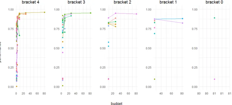
Figure 19a shows this problem while optimizing a neural network with Hyperband. Each dot in this plot represents a configuration at a certain state and bracket (the budget allocation). These interconnected dots are the configurations which were not sorted out immediately but retrained instead. Both rear brackets s= 1 and s= 0 sample predominantly “bad” configurations. The accuracy of each bracket’s best configuration are 0.962,0.953,0.939,0.881 and 0.89 (from s= 4 to s= 0). Hence, the most exploratory bracket s= 4 yielded the best performance.

In order to approach this problem, we propose to transfer information between each bracket. Figure 20 illustrates the basic idea. For Hyperband input parameters R = 81 and η = 3, we obtain a total of 5 brackets. The first one, s = 4, samples n = 81 configurations. Successive halving enables us to observe the behaviour for some of these configurations at different “budget stages”. Our central idea is to exploit this information and fit a surrogate model to learn

X |{z} conf igurations × _R |{z} budget → _R |{z} perf ormance (18) In particular, we want to use the most exploratory bracket as an initial design.

For the example of Figure 20, we know for at least n= 27 configurations how they performed with r0 = 1 and r1 = 3 units of budget. The best configurations of this bracket even contain 5 different values of ri.

Suppose we were optimizing neural networks and had a search space with three hyperparameters. The evolution of the best configuration’s accuracy in bracket s= 4 might look like this:

## optimizer learning.rate batch.normalization current_budget y

## 1 adam 0.05690947 TRUE 1 0.456

## 2 adam 0.05690947 TRUE 3 0.727

## 3 adam 0.05690947 TRUE 9 0.912

## 4 adam 0.05690947 TRUE 27 0.960

## 5 adam 0.05690947 TRUE 81 0.975

So for r0 = 1, the architecture obtains an accuracy of 45.6%. But for r1 = 3, the same configuration yields 72.7%. According to Equation 18, we utilize the budget as an additional hyperparameter. Furthermore, we take the complete brackets= 4 to represent our initial design.

(39)

Based on these, we want to propose n = 34 configurations for the subsequent bracket s= 3. In particular, we want configurations which are good for the maximum amount of resources in this bracket. So in order to conduct multi-point proposals, we need a purpose-built infill criterion. Actually invented to parallelize and therefore accelerate Bayesian Optimization, qLCB (Hutter et al. 2012) provides exactly what we need. Recall LCB from Equation 15. A simple trade-off between exploration and exploitation is controlled by a parameter λ. Now instead of one fixed value for λ, qLCB samples k different values λk from an exponential distribution. With

parameter 1

λ and expected valueλ we would like to sample:

qLCB(x, λk) = ˆµ(x)−λkseˆ(x), (19)

λk ∼Exp(1

λ), k = 1, ..., m

Each of these values forλk is optimized separately. In essence, low values ofλk mean exploitation

while high values on the other hand mean exploration.

Figure 19b shows the effect of this strategy on the same problem of Figure 19a. We see that the new sampling strategy avoids bad configurations in the rear brackets. In this particular example, the best performance was even observed in bracket s= 1 (accuracy of 0.973).

We call this method “Hyperband + MBO Budget”.

Supplementary, we want to propose two additional variants to combine Hyperband with MBO. For both of them, their surrogate models try to learn the simplified space

X |{z} conf igurations → _R |{z} perf ormance (20) The first of them which we call “Hyperband + MBO Mean” aggregates configurations based on their mean performance. Every configuration is weighted equally in the mean independent of the budget used for its evaluation. For instance, the configuration of the best model of bracket s= 4:

## optimizer learning.rate batch.normalization current_budget y

## 1 adam 0.05690947 TRUE 1 0.456 ## 2 adam 0.05690947 TRUE 3 0.727 ## 3 adam 0.05690947 TRUE 9 0.912 ## 4 adam 0.05690947 TRUE 27 0.960 ## 5 adam 0.05690947 TRUE 81 0.975 will be reduced to

## optimizer learning.rate batch.normalization y_mean.perf

## 1 adam 0.05690947 TRUE 0.806

The second modification “Hyperband + MBO Max” aggregates multiple occurring configurations by only using the best observed performance instead:

(40)

## optimizer learning.rate batch.normalization y_max

## 1 adam 0.05690947 TRUE 0.975

We will evaluate all of these mutations in chapter 5 on several problems.

(a) Optimizing a neural network with Hyperband. Here we suppose bad prior knowledge for some of our hyperparameters. Thus we have to deal with larger boundaries in our search space. Brackets= 1 ands= 0 issue a lot of resources on bad configurations. The best performance was achieved by brackets= 4, the most exploratory one (accuracy of 0.962).

(b) Optimizing a neural network with the combination of MBO and Hyperband on the same problem as Figure 19a. We utilized the budget as an additional hyperparameter (see Equation 18 and Figure 20). All brackets do now exhibit very similar performance values. The best performance was achieved by bracket

s= 1 (accuracy of 0.973)

(41)

Figure 20: Information transfer between Hyperband brackets. We want to utilize the configuration’s of bracket

s= 4 as our initial design. Equation 18 states that we also include each configurations budgetri as an additional hyperparameter for our surrogate model. Thus, we obtain an initial design with 81 + 27 + 9 + 3 + 1 = 121 configurations. Following up, a multi-point infill criterion will proposen= 34 configurations for the upcoming brackets= 3. After brackets= 3 has finished, we add these 34 + 11 + 3 + 1 = 49 configurations into our design. The design now contains 121 + 49 = 170 configurations. Hence, the configurations for brackets= 2 will be based on even more information than those of brackets= 3. Brackets= 1 on more thans= 2 ands= 0 on more thans= 1.

(42)

4 Implementation

One crucial part of this thesis was the implementation of the Hyperband algorithm. Since we planned further extensions of the original version, our central goal was to obtain a very generic variant. Therefore we opt for R6 (Chang 2017).

4.1 A Brief Introduction to R6

R6 is based on an encapsulated object oriented system, similar to those in Python or Java. In addition to data, objects do now contain methods. We can think of these methods as functions or “abilities” of the object. Using these methods enables us to directly modify the object. Suppose we would like to design an R6 class that creates objects for anytime algorithms. When initialized, the “algorithm objects” should contain a model as well as a method to continue the training of the model. The class could look like this:

algorithm = R6Class("Algorithm",

# The public argument is always a list and defines the interface of the object.

public = list( my.data = NULL, initial.budget = NULL, current.budget = NULL, init.fun = NULL, train.fun = NULL, model = NULL,

# To construct a new algorithm object, we have to call the $new() method. # It will automatically invoke the $initialize() method. Thus, to create an # algorithm object, we have to input four arguments:

initialize = function(my.data, initial.budget, init.fun, train.fun) { self$my.data = my.data

self$current.budget = initial.budget

self$model = init.fun(self$my.data, self$current.budget) self$train.fun = train.fun

},

# For an arbitrary budget, the $train method will call the train.fun:

train = function(budget) {

self$model = self$train.fun(self$model, self$my.data, budget) self$current.budget = self$current.budget + budget

} ) )

By calling the $new() method, we can create algorithm objects. The main ingredients are the init.fun, a function to initialize models and a train.funto access the train method:

(43)

myAlgorithmObject = algorithm$new(my.data = my.data,

initial.budget = 10,

init.fun = init.fun,

train.fun = train.fun)

This is were the advantage of R6 manifests itself. We chose an init.fun such that we obtain a boosting ensemble from the XGBoost package (Chen et al. 2018):

myAlgorithmObject

## <Algorithm> ## Public:

## current.budget: 10

## initialize: function (my.data, initial.budget, init.fun, train.fun) ## model: xgb.Booster

## my.data: xgb.DMatrix ## train: function (budget)

But we could have chosen anything else, such as a neural network from the MXNet package (Chen et al. 2017) in combination with mlr (Bischl et al. 2016). All we have to change are our

init.fun and train.fun: myOtherAlgorithmObject

## initialize: function (my.data, initial.budget, init.fun, train.fun) ## model: classif.mxff from package mxnet

## my.data: list

## train: function (budget)

By calling the train method, we directly manipulate the object. That means that we alter the current.budget, but in particular, the state of the model.

myAlgorithmObject$train(20)

## initialize: function (my.data, initial.budget, init.fun, train.fun) ## model: xgb.Booster

## my.data: xgb.DMatrix ## train: function (budget)