Mersland, R. and Strøm, R. Ø. (2010),
“Microfinance Mission Drift?”
World Development. Vol. 38(1), pp. 28-36.
1
Microfinance mission drift?
Roy Mersland
University of Agder, Kristiansand, Norway
R. Øystein Strøm
Østfold University College, 1757 Halden, Norway
Abstract
Claims have been made that microfinance institutions (MFIs) experience mission drift as they increasingly cater to customers who are better off than their original customers. We investigate mission drift using average loan size as a main proxy and the MFI’s lending methodology, main market, and gender bias as further mission drift measures. We employ a large data set of rated, multi-country MFIs spanning 11 years, and perform panel data estimations with instruments. We find that the average loan size has not increased in the industry as a whole, nor is there a tendency towards more individual loans or a higher proportion of lending to urban costumers. Regressions show that an increase in average profit and average cost tends to increase average loan and the other drift measures. More focus should be given to cost efficiency in the MFI.
2
1 Introduction
The microfinance industry is coming of age, and with its maturation have come claims that the industry is abandoning its mission to serve the poor (Dichter and Harper, 2007). According to Nobel Peace Prize winner Muhammad Yunus, clients who are financially better off crowd out poorer clients in any credit scheme (Christen and Drake, 2002 p. 10). The mission of all
microfinance institutions (MFIs) is to provide banking services to the poor, that is, to lend very small sums to very poor borrowers. The objectives of this paper are first to determine the extent of mission drift, and second, to provide explanations for why mission drift does or does not occur.
Financial viability is a major concern for the industry. A recent survey conducted by the MicroBanking Bulletin (autumn 2007) based on the THEMIX 2006 benchmark data set of 704 MFIs reveals that 41% are not financially self-sustainable; they rely on donor support to keep afloat. However, in pursuing financial objectives, there is the risk of losing sight of social objectives. Ever since PRODEM, a Bolivian non-governmental MFI, was commercialized and transformed into the shareholder-owned Banco Sol in 1992, addressing the risk of mission drift has been high on the industry’s agenda (Rhyne, 1998). Recent events, such as the initial public offering of Banco Compartamos in Mexico that led to a handful of people making a USD 450 million fortune, have added steam to the debate (Rosenberg, 2007).
Thus, some critics fear that MFIs become too focused on making profits at the expense of outreach to poorer customers. The argument is that higher profits lead to lower outreach. However, Rhyne (1998) and Christen and Drake (2002) conjecture that a more commercialized microfinance industry is better able to serve the poorest members of the community, since their
3
profit motives lead them to be more efficient and more willing to seek out new markets for their loan products. The implication is that when we seek explanations for mission drift, we should focus upon the MFI’s costs as well as its profits. In this paper, we address these issues in the framework of a bank’s profit function freixasrochet2008, where we also include the MFI’s risk. Preliminary empirical evidence supports the Rhyne (1998) and Christen and Drake (2002) position. Hishigsuren (2007) thoroughly analyzes one MFI in Bangladesh using archival, survey, and interview data from different stakeholders. This important case study concludes that the MFI shows no statistically significant mission drift when measured by depth, quality, and scope of outreach to poor clients, at the same time that the MFI is able to achieve greater cost efficiency. In country studies, Paxton et al. (2000) argue that there is a trade-off between serving the poorest segments and being financially viable, since transaction costs associated with smaller loans are high when compared to those associated with larger loans. However, in a study of commercialized and transformed MFIs in Latin America, Christen (2001) concludes that mission drift has not taken place. Littlefield et al. (2003) find that programs that target very poor clients perform better than others in terms of cost per borrower, an efficiency indicator that neutralizes the effect of smaller loan size. Fernando (2004) analyzes 39 transformed MFIs and finds that their financial positions improved significantly and they did not lose sight of their mission. Both case and country studies lack generality. Until now, Cull et al. (2007) is the only larger cross-country study to address mission drift. Using a sample of 124 MFIs in 49 countries, they find that MFIs can stay true to their mission even when they aggressively pursue financial goals. Our study differs from theirs in that the data material is larger, we use instruments in estimation, and our study is specifically geared towards the mission drift question.
Woller et al. (1999) and Woller (2002) hold that mission drift occurs when an MFI leaves the poor customer segment. We subscribe to this view, to which there seems to be general
4
customers, its depth dimension of outreach (Schreiner, 2002), is weakened. Depth outreach concerns the MFI’s provision of financial services to the poorest segments, and is first and foremost defined as average loan as in Cull et al. (2007), but depth outreach also includes the extent of lending in rural communities, to women, and lending through group loans (Bhatt and Tang, 2001). This paper gives characteristics of outreach measures, and provides explanations for mission drift using panel data regression estimations with the generalized method of moments (GMM) for average loan and logistic regressions for the other depth measures. The GMM methodology enables estimations without endogeneity bias, and, since we use a set of country variables in the instrument set, country effects are neutralized.
Despite the interest that has been expressed in mission drift, few studies have been carried out to examine the issue, even fewer rigorous empirical studies. ”Since relatively few rigorous studies on the impact of microfinance have been completed, ideology tends to dominate’’ the
debate on misson drift, a New Yorker article by Bruck (2006) runs. In this paper we intend to
replace ideology with analysis. The ongoing debate and the lack of cross-country studies involving a large number of MFIs indicate a need for our study. We address mission drift explicitly using data from rated MFIs in 74 countries.
We test three main hypotheses for mission drift derived from Freixas and
Rochet (2008): profitability per customer, costs per customer, and customer risk. The first two hypotheses imply that an MFI will increase the size of its average loan in order to improve financial results, while risk is uncertain. The MFI may limit risk by making smaller loans, or by migrating to customers who are better off. The first strategy implies a smaller average loan size, the second a larger.
The data set used to conduct this study includes observations of 379 MFIs in 74 countries collected by rating agencies during the years 2001 to 2008. Since the data were collected by third parties, they are more reliable than self-reported data. We find no evidence of mission
5
drift in the industry as a whole; however, panel data estimations using GMM reveal that the size of the average loan increases with increased average profit and average cost. These results imply that mission drift may occur if an MFI seeks higher financial returns, but that this effect is neutralized if the MFI is more cost efficient. These results confirm the Rhyne (1998) and Christen and Drake (2002) conjecture. Furthermore, we find that average cost is more important than average profit in determining average loan size. Though profit seeking leads to mission drift, attention should be given to reducing an MFI’s costs.
The remainder of this paper proceeds as follows: In section 2, we describe our data on rated MFIs. In section 3, we discuss what we mean by mission drift and provide descriptive statistics. The aggregate data show no signs of mission drift. In section 4, we develop our theory and hypotheses. Section 5 provides an overview of the panel data methods used. The hypotheses are tested in section 6, and our conclusions are presented in section 7.
2 Data
Our study is based on observations of 379 rated MFIs in 74 countries. Third-party organizations established the standardized ratings, and outside organizations subsidized part of the costs involved (www.ratingfund.org). The main motive for an MFI to submit to a rating is improved access to external funding. The third-party and standardized MFI data collected from the rating agencies is judged to be better than self-reported data as found, for instance, in the Mixmarket database. The data set includes both financial and outreach data, and is thus well suited for studying the mission drift issue.
At each rating, four years of data were commonly obtained, although some MFIs report five and six years of data. The rating agency obtains data for the current year as well as for
immediately preceding years when visiting. The method of data collection means that the panel of data is highly balanced. This means that we have 1,159 observations for average loan and a
6
similar number for other variables in the analysis. The ratings were performed from 2001 to 2008, which means that we have data from 1998 to 2008, with more than 100 observations for each year from 2001 to 2006. The variables used in the analysis are defined in table 1.
Table 1
The index number problems associated with country specific effects make comparisons
between countries difficult (Deaton, 1995). We alleviate these problems by several procedures. First, we convert the monetary variables into USD at the going exchange rate, and then adjust them for purchasing power parity (PPP) bias based on IMF data. According to the purchasing power parity principle in international finance (Solnik and McLeavey, 2004) the first step means that country inflation rates are reflected in the exchange rate. However, conversion by market rates only is criticized for not taking account of the true purchasing power in the local market. The IMF’s GDP-PPP is an attempt to correct for this. By adjusting with this index, we make each loan (and each local cost) more comparable across nations. Second, we use country variables as instruments in the regressions. Third, panel data statistical methods, specifically the fixed effects method, remove time invariant and idiosyncratic differences from the data
(Woolridge, 2002).
3 Mission drift
The average loan is the most commonly used indicator among microfinance investors and donors to measure the degree of MFI outreach to poor customer segments (Bhatt and Tang, 2001; Cull et al., 2007; Schreiner, 2002). Mission drift occurs when the size of the average loan increases. This indicates that an MFI has moved into new customer segments, either because it begins to include customers who are better off or because existing clients experience success and are thus able to take on larger loans. In Schreiner (2002) average loan is one proxy for the
7
First, increasing the depth of outreach means reaching more women. Outreach to women has been a priority almost since the inception of Grameen bank (Dowla and Barua, 2006). Second, group lending has been the cornerstone of microfinancing. Instead of requiring formal
collateral, loans are backed by peer groups (Armendariz de Aghion and Morduch, 2005; Ghatak and Guinnane, 1999). Therefore, a shift from group lending to individual lending leads the MFI away from uncollateralized lending necessary to reach the poorest customers and may bring about mission drift and a reduction in the overall developmental impact stemming from group participation (Thorp et al., 2005). Third, reaching rural areas is a significant goal in
microfinance, since this is where poverty is most concentrated (United Nations, 2006). When the relative weight of loan allocation shifts to the urban market, mission drift occurs.
Table 2 provides an overview of the depth characteristics. Table 2
The table shows that the average loan is less than USD 750, and the median is as low as USD 332 in PPP-adjusted terms. Thus, the loans are on average small. The growth rate at the bottom of the table shows that the average loan in 2007 is smaller than the average loan in 1999. This may come about either because each individual MFI reduces the average loan, or because MFIs that have a higher proportion of smaller loans are rated late in the sample period.
The lending methodology summarized in the ”Group’’ column shows that individual loans are the most common, but that group lending is increasing in the period. In fact, the average loan size is USD 1,134 for individual loans, USD 177 for village loans and USD 401 for the solidarity group. More group lending can be an explanation for the near constant average loan size in the period. The main market variable ”Rural’’ also shows an increase in depth outreach. However, the MFI’s gender bias is smaller, thus, the MFIs on average report a lower preference for female clients. All in all, the various measures do not add up to a confirmation of the
8
Let us look closer at the average loan. A mission drift for the individual MFI would be
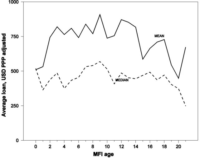
indicated if there were an increase in average loan size relative to the MFI’s starting year. Thus, older MFIs should service larger loans if mission drift is the case. We have removed average loans higher than USD 10,000 (PPP-adjusted) from the sample in order to prevent outliers influencing the average. This gives a loss of 9 observations out of 1,159 for average loan, or 0.8 per cent of the sample. Figure 1 confirms findings in table 2.
Figure 1
Figure 1 depicts both the mean and the median average loan, so as to avoid the impact of a few high average loans in a given year. Both series show that average loan size does not increase with the MFI’s experience. Rather, the trend is downward over the years. Given that the International Monetary Fund’s (IMF) records of the developing countries GDP per capita PPP-adjusted shows an increase from USD 2,834 to USD 5,588 or 97.1 per cent in the period 1998 to 2008, the non-rise of the average loan is even more remarkable. Replacing the average loan in figure 1 with the mean average loans for each MFI, we again obtain that average loan does not rise with MFI age. Thus, evidence from aggregate data cannot confirm the claim that as MFIs get older, they tend to drift from its original mission, thus leading to lower outreach.
3 Mission drift: Theory and hypotheses
We now develop hypotheses to explain the apparent lack of mission drift. The assumption is that all MFIs need to be financially sustainable in order to continue business. Thus, the decision to stay in an initial market segment or to allow a drift into a new segment is guided by
consideration of profits. Thus, we may focus upon the MFI’s profit function alone. This also allows the severest test in favor of the mission drift argument.
Disregarding governance issues, assume that an MFI is risk averse with an exponential utility
9
is its measure of risk aversion. When profits are normally distributed, the expected utility of profits may be written:
𝐸 𝑢 𝜋 = 𝑢 𝜋 −1
2𝜌𝜍2 = 𝑢 𝑃
Here, 𝜍 is the risk of profits. Thus, in order to maximize expected utility, the MFI should
maximize P.
We need to specify P to arrive at an estimable function. As a first step, consider the bank’s
profit function 𝜋 (Freixas and Rochet, 2008):
𝜋 𝐷, 𝐿 = 𝑟𝐿−𝑟 + 𝑟 1 − 𝛼 − 𝑟𝐷 𝐷 − 𝐶 𝐷, 𝐿 ,
where 𝑟𝐿 is the rate of loans, 𝑟𝐷 is the rate of deposits, r is the rate on the interbank market, L is
loans, D is deposits, 𝛼 is the percentage of deposits for compulsory reserves, and C(D,L) is the
production function or management costs. The bank’s profit is the sum of the intermediation margins on loans and deposits, net of management costs. The risk of profits is composed of risk in the intermediation margins, changes in the demand for loans and supply of deposits, the repayment on loans, and management cost risk. For now, we assume that for an MFI the chief risk lies in repayment.
Three arguments for this can be laid down. First, the MFI may be able to maintain near constant intermediation margins, even though the loan rate on the interbank market is variable. This is the case when the MFI is the sole provider of financial services in its area, and therefore, has some degree of monopoly power over customers. Then the MFI is able to control its own risk level (Freixas and Rochet, 2008, p. 8991). Furthermore, relationship banking is a characteristic of microfinance. In such a setting, the customer becomes locked in with the bank (Sharpe, 1990; Rajan, 1992; Mersland, 2009). The MFI has some power to fix deposit and lending rates, and is therefore able to neutralize changing rates on the interbank market. Second, an MFI’s management cost is primarily related to labor. These should be predictable and thus contain small risk. Third, repayment costs are likely to be risky even though microfinance observers
10
find that the poor repay their loans. MFIs try to minimize their losses by making small loans with short maturity terms; by making group loans, so that peers control each other; and by differentiating between individuals based on their reputations as their individual credit histories accumulate (Ghatak and Guinnane, 1999). Nonetheless, repayment seems to be the chief risk element in microfinance, since an MFI is often unable to differentiate between good and bad risks and to monitor a client’s performance (Armendariz de Aghion and Morduch, 2005). The upshot is that only repayment risk remains, leaving us with:
𝑃 = 𝑟𝐿−𝑟 𝐿 + 𝑟 1 − 𝛼 − 𝑟𝐷 𝐷 − 𝐶 𝐷, 𝐿 −
1
2𝜌𝜍2 𝐿 ,
where 1 𝜌2 is a constant. We see that P is a risk-adjusted profit measure and assume that the
management cost function is linear. By a simple rearrangement of the last equation and a
division by the number of credit clients, CC, the average loan 𝐿 may be written:
𝐿 = 1 𝑟𝐿− 𝑟 𝑃 𝐶𝐶− 𝑟 1 − 𝛼 − 𝑟𝐷 𝑟𝐿− 𝑟 𝐷 𝐶𝐶+ 1 𝑟𝐿− 𝑟 𝐶(𝐷, 𝐿) 𝐶𝐶 + 1 2𝜌𝜍2 𝐿
The right-hand side shows (risk adjusted) profit, deposits, management costs, and loan risk per credit client. The model yields the predictions that average loan size will increase with higher profits, lower deposits, higher management costs, and higher risk per credit client. Notice that the intermediation margins are the same for average profit and average cost. If the signs are equal, but coefficients differ, either average profit or average cost will be the more important variable. Testing takes this last equation as the point of departure. However, it raises problems of endogeneity, which we address using instruments, see section 5.
The prediction for risk indicates that higher risk per customer may lead to mission drift, since the bank may then favor higher loans to members of society who are better off. This is a mission drift hypothesis. However, a risk exposure argument would result in the opposite prediction. When risk per customer increases, one would expect MFIs to reduce the average loan size. After all, this is one of the ways any bank uses to limit risk exposure to particular
11
customers. This is a risk exposure hypothesis. Thus, the risk prediction in the last equation is not clear-cut.
In addition to the model variables, an MFI’s time in business may induce it to accept smaller loan sizes. This time variable is important, since the mission drift argument implies that the older an MFI, the more it will drift towards higher income segments. Figure 1 demonstrates that the average loan size for all MFIs does not increase with MFI age. Two effects pulling in the same direction may be at work here. The first is a cost effect in which operating costs may drop over time as an MFI expends less effort to promote microloans and to ensure their repayment. The second effect stems from the fact that a repeat relationship with the same customer segment reveals its typical creditworthiness. An MFI may be willing to extend marginal and smaller loans deeper into a segment with a good record. The initial low-risk customers in a given segment may establish a good reputation, which benefits followers with lower loan demands. An experienced MFI is more likely than a novice to obtain such customer information and to risk lending to smaller customers.
The hypotheses are summarized in table 3, together with descriptive statistics on variables that enter the analysis.
Table 3
As we have noted, average loans higher than USD 10,000 (PPP-adjusted) constitute 0.8 per cent of the sample. Since these outliers may influence regression results, they are removed in
estimations. We use only the MFI’s assets as a control variable because the many country instruments (see section 5) will act as controls.
McIntosh and Wydick (2005) suggest that increased competition among MFIs may lead to mission drift when cross-subsidiation of the weakest customers becomes less feasible. They assume that MFIs compete in a market with a fixed number of customers. However, the effects of competition is mediated through the profits. Thus, profits constitute the final step in the
12
argument leading to mission drift. This variable is already in our setup. Furthermore, the
assumption of a fixed number of customers is clearly not realistic in the microfinance market. If anything, the rapid increase in the customer base is a characteristic of microfinance. In fact, in our sample the yearly growth rate of credit clients is 44.2 per cent in 875 observations. This growth gives hopes that the MFIs are able to achieve large scale advantages. Therefore, both profits and cost advantages are covered in our estimations.
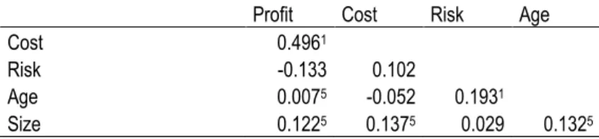
Table 4 shows the correlations between the explanatory variables. We include this table to facilitate a discussion of the potential multicollinearity among the independent variables. Table 4
The table shows a number of significant bivariate correlations among the averages of our
explanatory variables. For instance, average cost is significantly correlated to average profit and to firm size, measured as assets. However, these, and all other correlation coefficients, are rather low. Kennedy (2008, p. 196) notes that correlations need to be in the area of 0.8 to 0.9 to detect collinearity among two variables. None of the correlation coefficients in the table are in this range.
5 Tests and methods
We implement our estimates when average loan is the dependent variable and the independent variables’ hypotheses set out in table 3. In addition to the variables, the panel data includes a fixed effects error term together with a pure error term. The fixed effect, or time invariant, error term contains unobserved effects, such as the MFI’s “way of doing things”. We include country instruments in estimations, see below, which neutralize country effects.
The same independent variables are used for the other mission drift variables, that is, lending methodology, main market, and gender bias.
13
Before we proceed to estimation we should check if panel data estimation is really necessary, or if the variations for each MFI are so small that pooled regressions suffice. An ANOVA test (Hsiao, 2003, ch. 2) reveals individual, time, and joint effects in our panel data. The ANOVA
analysis uses the individual (i) and time (t) residuals of the pooled OLS regression. The
ANOVA test is a test of whether the regression slopes are homogeneous for all individual MFIs
at all times. The results of F tests of individual, time, and joint effects, show that all effects are
significant at the 1% level, thus rejecting the homogeneity assumption across MFIs and time. The test indicates that a pooled OLS regression is inappropriate, and that we should use panel data estimation (Woolridge, 2002).
A difficulty in estimation is that the profit, cost, and risk variables are determined
simultaneously with average loan. Thus, the relation suffers from an endogeneity bias. The bias may be removed in the statistical sense if we can find a set of relevant instruments that are
independent of the error term. We need at least as many instruments (L) as regressors (K) in
order to identify the coefficients 𝛽𝑗, (𝑗 = 1, ⋯ ,5). Fortunately, panel data provide a wealth of
opportunities for constructing instruments, far more than in a simple cross-sectional analysis (Deaton, 1995). We find instruments among country specific variables and the lagged explanatory variables. Since our choice results in the number of instruments exceeding the
number of regressors 𝐿 > 𝐾, we have a set of overidentifying restrictions. The instruments’
independence of the error term is then tested with the Hansen (1982) J test which is distributed
as 𝜒2(𝐿 − 𝐾), where (L-K) is the degrees of freedom. A high value indicates that at least some of the instruments are correlated with the error term, and thus, endogeneity in the statistical sense is not removed.
We find instruments among country specific variables and the lagged explanatory variables for the estimation. The country variables are the IMF data on GDP per capita (adjusted for
14
GDP, and finally, the overall Heritage Foundation index of economic freedom. For all these series, yearly records for the needed period from 1998 to 2008 are kept for nearly all countries. For new Balkan countries we use records for neighbors, if the country records are missing. The instruments will neutralize country specific effects, whether these are due to wealth level, growth, and risk. The economic freedom index includes measures for the individual’s freedom to enter into contracts (for instance, to invest), as well as measures for the government size and the country’s level of corruption. Thus it also contains important country institutional
conditions in addition to the macroeconomic conditions from IMF. The World Bank’s Doing
Business index is an alternative to the economic freedom index, however, the index starts only
in 2004.
The country instruments are generally weak. We supplement with lagged explanatory variables as instruments. This is possible because the independent variables are all simultaneous, and therefore, the lagged variables are unrelated to average loan. However, the lagged variables should be related to the explanatory variable.
We perform estimations using the GMM estimator. With the optimal weighting matrix the GMM estimator allows for arbitrary heteroskedasticity and serial dependence when the number
of MFIs N is large, and the number of time periods T is low (Woolridge, 2002, p. 193-4). This
is fulfilled here, since we have 379 MFIs and 𝑇 = max𝑇6.
We use three different panel data methods, fixed effects, random effects, and first difference. The fixed-effects panel data estimation amounts to subtracting the individual MFI averages from the annual observation, and performing regression on these transformed variables. The procedure removes individual MFI heterogeneity, since fixed effects are assumed constant during the observation period. For instance, an MFI’s country identity is assumed fixed. Thus, the fixed effects are removed together with the constant. The random-effects estimation is performed by assuming that the fixed effect error is part of the error term. We implement this
15
by running first a generalized least squares (GLS) regression, obtain the variances, and use these for data transformation and final estimation with GMM. The first-difference estimation
methodology involves the change in average loan due to change in profit per loan client and
other variables. This means that the difference in average loan, 𝐿 𝑡− 𝐿 𝑡−1, is regressed on
similar differences in explanatory variables. Again, the fixed effects and the constant are removed. Together, the three panel data regressions should increase our faith in the results if their coefficients are similar and significant.
6 Econometric evidence
The estimation strategy is to first estimate our relation with average loan as the dependent variable using the three panel methods: fixed-effects, random-effects, and first-difference, and then to use the same explanatory variables for lending methodology, main market, and gender bias in logistic regressions.
6.1 The average loan
The country effect instruments GDP-PPP per capita, GDP growth, inflation, the current account balance as a percentage of GDP, and the economic freedom index are transformed, so that for instance in fixed effects estimations the instruments are demeaned. The explanatory variables making up the rest of the instruments are in original levels and lagged one period. Since we also use a constant as an instrument, this gives six overidentifying restrictions for fixed effects and first difference methods, and five for random effects.
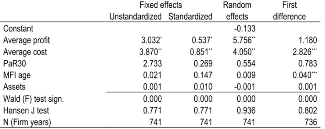
The results of estimating the regression for average loan are shown in table 5. Table 5
Notice that a regression on standardized values (average zero and standard deviation equal to 1.0 for all variables) is included. Disregarding this for the moment, we observe that average
16
profit and average cost are significant and equally signed in all panel data estimations. Thus, the results from the different panel data estimation methods are largely consistent, adding
credibility to the results. Furthermore, the overall Wald statistics are very satisfactory, and the
Hansen J statistic of overidentifying restrictions shows that instruments are not correlated with
the error term. Thus, the instruments are relevant.
Taking a closer look, we note that the profit per loan client is positive in the fixed and random-effect panel data regressions, indicating that the average loan size increases with the profits per loan client. This result confirms the hypothesis of the relationship between average profit and average loan from the Freixas and Rochet (2008) model. Thus, an MFI is able to earn a larger absolute profit with a larger average loan size. This has the potential to support Yunus’s proposition that clients who are better off crowd out poorer clients in any credit scheme (Christen and Drake, 2002, p. 10). If an MFI demands higher profits per client, the poorest customers tend to be driven away.
Table 5 also shows that the average loan size increases with costs per loan client in all regressions, confirming a further hypothesis based on the model developed by Freixas and Rochet (2008). Thus, inefficient MFIs need to shift their loan portfolios toward larger average loans. This means that inefficient MFIs are those most susceptible to mission drift. Another implication is that when an MFI increases its cost efficiency, it is better able to advance loans to the poorer members of the community. This result is in line with the observation made by Hishigsuren (2007) that the MFI in her case study increased lending to the poor, even when the time a lending officer spent with a borrowing group was cut in half. It also confirms the cost findings in Littlefield et al. (2003).
Thus, average profit and average cost have a significant impact on average loan size. Which one is the most important? The regression with standardized values allows comparisons of importance. It shows that the economic effect of average cost is more important than average
17
profit. If an MFI is able to increase its average profit by one standard deviation, the size of the average loan will increase by about 54%, and will increase by about 85% with a similar change in average cost. Conversely, this also implies that when an MFI is run more efficiently, the MFI is able to reduce average loan size and prevent mission drift. If an MFI tends to increase cost efficiency more than average profit, we should not expect mission drift.
The PaR30 risk hypothesis is uncertain, and the uncertainty is confirmed by no significant results in estimations. Thus, we cannot decide if the exposure effect of risk is stronger than the mission drift effect. For the MFI’s age the positive and significant result in table 5 means that when other variables are taken into consideration, the individual MFI tends to increase the average loan size with time. However, this result obtains in only one regression.
In unreported regressions, we run several robustness checks. First, we test if the intermediation margin risk affects our estimates. A measure of such a risk is the inverse of the cost of funds divided by the portfolio yield. The higher this is the higher the risk. However, we find no effect from this measure. If we allow intermediation margin risk to enter, we should also check for its correlation with our preferred risk measure, PaR30. However, this is very low and not
significant. We also calculated the Z risk measure (Berger et al., 2008) given by 𝑅𝑂𝐴𝑖 +
𝐸𝑖/𝐴𝑖 /𝜍𝑅𝑂𝐴𝑖, where the subscript denotes MFI number i, ROA is the return on assets, 𝜍𝑅𝑂𝐴𝑖is
its standard deviation, E is equity, and A is the MFI’s total assets. The lower is Z the higher its
probability of default. Using this measure instead of or in addition to PaR30 did not bring any material changes to the regression results. The same applies to the risk measures debt-equity ratio and the ratio of voluntary savings to loans. Last, we use deposits instead of operational costs per loan client, and obtain essentially the same results for profits per loan client as those shown in table 5. The results for the other variables remain largely unperturbed. Thus, our regression results are robust to different variable specifications.
18
6.2 Leaving the group borrowers, the villages, and the women?
If mission drift is the case among MFIs, one should expect MFIs to place less weight upon group lending, lending to rural customers, and to women. These alternative measures of the depth dimension in outreach (Schreiner, 2002) may provide further robustness tests of our results.
We use logistic regressions in this section (Woolridge, 2002, p. 453...). The reason is that lending methodology, market, and gender bias are all categorical variables. For the two first, more than two categories exist. We convert these into indicator variables. For lending
methodology this means that 1 signifies individual loan, and 0 other lending arrangements, such as group lending through a village bank. The MFI’s main market is 1 if it gives mainly to urban customers, 0 otherwise. These variables are time invariant, thus, an MFI is supposed to keep its characteristics as a lender to groups or rural customers throughout the four or five years for which we have observations.
The time invariance places restrictions on the estimation techniques available. Fixed effects estimation is no longer possible, and random effects may be doubtful since it requires stringent assumptions. We decide to pool the data, add the country instruments as control variables, and furthermore, to include year dummy variables in regressions. Moreover, correcting for
endogeneity is difficult in binary choice models (Woolridge, 2002, p. 490). Accordingly, we estimate without instruments. Since the new depth measures do not follow from the original relation, it is not certain that endogeneity corrections should be made.
The results from the pooled logistic regression are set out in table 6. Table 6
The table confirms the result for average loan in the former section. In particular, average cost turns out to be significant for all three variables and has the same sign as in average cost regressions. Thus, higher average cost will induce the MFI to seek more individual customers,
19
customers in urban communities, and to focus less on female customers. The reverse of this is of course that to the extent that the MFI is able to keep costs down, it is able to serve group, rural, and female borrowers. Furthermore, the average profit is significant for lending methodology only, thus confirming the weaker result for average profit than average cost in table 5. In these new regression we find risk is significant two times. Thus, a higher repayment risk means that MFIs lend more to individuals and assume lower bias for female customers. We perform logistic regressions with random effects panel data and with the average values for each MFI as simple robustness tests. In both, the country variables are kept as instruments, but year indicator variables are dropped. Except for main market, the results in both types of estimation parallel those in table 5.
7 Conclusion
Some commentators fear that as microfinance is becoming more ”commercialized’’, the microfinance institution (MFI) will drift away from its original goal of providing financial services to the poor. ”The Yunus faction worries about ”mission drift’’, saying that, as the drive for profitability increases, only the so-called ”less poor’’ (as opposed to the very poor) will qualify for loans’’ says Bruck (2006). On the other hand, Rhyne (1998) and Christen and Drake (2002)hold that the profit motive leads MFIs to seek out new markets and to be more efficient. We are able to enlighten the debate using data from rated MFIs in 74 countries for the period from 1998 to 2008, supplying both descriptive and econometric evidence from panel data estimations on mission drift.
Our main conclusion is that we cannot find evidence of mission drift. This is in line with the Rhyne (1998) and Christen and Drake (2002) conjecture that profits and costs may outweigh each other and thus not lead to mission drift or lower outreach. Building upon a bank profit function framework (Freixas and Rochet, 2008) we hypothesize that profit per credit client is
20
correlated with average loan amount. The econometric evidence supports this hypothesis as general methods of moment (GMM) estimations with panel data methods and instruments show that average loan size increases with an increase in average profits and average operational costs. The impact of MFI risk upon the size of the average loan is undecided. Furthermore, logistic regressions with lending methodology (group or individual), main market (rural or urban), and gender bias support the findings for average loan. Together with the descriptive evidence, this shows that the MFIs tend to maintain and even increase the depth outreach of average loan. These results confirm the findings of the few prior studies that have focused on mission drift (Littlefield et al., 2003; Cull et al., 2007; Hishigsuren, 2007), and they repel the Yunus worry, perhaps because Yunus reasons in a static framework, whereas the dynamism in MFIs’ cost reductions countervails the tendency for higher average loan.
Thus, the more cost effective an MFI is, the smaller the average loan. A prediction can thus be made that further efforts to reduce costs will result in MFIs reaching out to even poorer
segments, when profitability is at the same level. Rather than concentrating on an MFI’s ”commercialization,’’ attention should be focused on how to reduce costs per client. Since the microfinance industry is still young and growing strongly, there should be room for cost reductions in the future. Better management may provide MFIs with good economic reasons to stay in the poorer customer segment.
By using average loan as our main outreach variable we follow common practice among researchers (Bhatt and Tang, 2001; Cull et al., 2007; Schreiner, 2002) as well as practitioners, investors, and donors. There are however weaknesses in using an average value. Our alternative measurements individual loan, female clients and rural market are thus important to include. We also welcome other mission drift studies using other data and alternative outreach
measurements such as for instance percentage of MFI-clients below a PPP defined threshold or average loan for new customers.
21
There is a need for more efficiency studies to better understand cost drivers in MFIs. It is possible that specialized, credit-only MFIs, or partnerships with regular banks to facilitate savings mobilization, are more customer-friendly strategies than the current recommendation urging MFIs to become fully fledged banks (Helms, 2006). Furthermore, there is a need for rigorous studies of the several MFIs that have transformed from being non-profit to becoming for-profit. Have these left their mission to serve the poor? We hope to address these issues in future studies.
22
References
Armendariz de Aghion, B. & Morduch, J. (2005). The Economics of Microfinance.
Cambridge: MIT Press.
Berger, A.N., Klepper, L.F. & R.Turk-Ariss (2008). Bank competition and financial stability.
Policy Research Working Paper 4696, The World Bank.
Bhatt, N. & Tang, S.-Y. (2001). Delivering microfinance in developing countries:
Controversies and policy perspectives. Policy Studies Journal29, 319-333.
Bruck, C. (2006). Millions for millions. The New Yorker, Oct issue.
Christen, R. & Drake, D. (2002). Commercialization. The new reality of microfinance.
In D.Drake & Rhyne, E. (Eds.). The Commercialization of Microfinance. Balancing Business
and Development, (pp. 2-22). Bloomfield: Kumarian Press.
Christen, R.P. (2001). Commercialization and mission drift. Occasional Paper. Washington
DC: CGAP.
Cull, R., Demigüc-Kunt, A. & Morduch, J. (2007). Financial performance and outreach: A
global analysis of leading microbanks. Economic Journal 117(517), 107-133.
Deaton, A. (1995). Data and econometric tools for development analysis. In J.Behrman & T.
Srinivasan (Eds.), Handbook of Development Economics, Volume3A of Handbooks in
Economics (pp. 1785-1882). Amsterdam: Elsevier.
Dichter, T.W. & Harper, M. (2007). What’s wrong with microfinance. In T.W. Dichter & M.
Harper (Eds.), What’s wrong with Microfinance. Essex, England: Practical Action Publishing.
Dowla, A. & Barua, D. (2006). The Poor Always Pay Back. The Grameen II Story.
Bloomfield, USA: Kumarian Press, Inc.
Fernando, N.A. (2004). Micro success story, transformation of nongovernmental organizations
23
Freixas, X. & Rochet, J.-C. (2008). Microeconomics of Banking (2nd ed.). Cambridge, Mass.:
MIT Press.
Ghatak, M. & Guinnane, T.W. (1999). The economics of lending with joint liability: Theory
and practice. Journal of Development Economics 60, 195-228.
Greene, W.H. (2003). Econometric Analysis (5th ed.). New York: Prentice Hall.
Hansen, L.P. (1982). Large sample properties of generalized method of moments estimators.
Econometrica50(4), 1029-1054.
Helms, B. (2006). Access for All: Building Inclusive Financial Systems. Washington DC:
CGAP.
Hishigsuren, G. (2007). Evaluating Mission Drift in Microfinance: Lessons for Programs With
Social Mission. Evaluation Review31(3), 203-260.
Hsiao, C. (2003). Analysis of Panel Data (2. ed.). Cambridge: Cambridge University Press.
Keeney, R.R. & Raiffa, H. (1993 (1976)). Decisions with Multiple Objectives. Cambridge:
Cambridge University Press.
Kennedy, P. (2008). A Guide to Econometrics (6th ed. ed.). Oxford, UK: Blackwell Publishing.
Littlefield, E., Morduch, J. & Hashemi, S. (2003). Is microfinance an effective strategy to reach
the millennium development goals? CGAP: Focus Note No. 24, Washington DC.
McIntosh, C. & Wydick, B. (2005). Competition and microfinance. Journal of Development
Economics 78, 271-298.
Mersland, R. (2009). The cost of ownership in microfinance organizations. World Development
37(2), 469-478.
Paxton, J., D.Graham, & C.Thraen (2000). Modeling group loan repayment behavior: New
insights from Burkina Faso. Economic Development and Cultural Change 48(3), 639-55.
Rajan, R.G. (1992). Insiders and outsiders: The choice between informed and arm’s-length
24
Rhyne, E. (1998). The Yin and Yang of microfinance: Reaching the poor and sustainability.
MicroBanking Bulletin 2, 6-9.
Rosenberg, R. (2007). CGAP reflections on the Compartamos initial public offering: A case
study on microfinance interest rates and profits. Focus Note 42, Washington DC: CGAP.
Schreiner, M. (2002). Aspects of outreach: A framework for discussion of the social benefits of
microfinance. Journal of International Development 14, 591-603.
Sharpe, S.A. (1990). Asymmetric information, bank lending, and implicit contracts: A stylized
model of customer relationships. Journal of Finance 45(4), 1069-1087.
Solnik, B. & D.McLeavey (2004). International Investments (5. ed.). London: Pearson Addison
Wesley.
Thorp, R., Stewart, F. & Heyer, A. (2005). When and how far is group formation a route out of
chronic poverty? World Development 33, 907-920.
United Nations (2006). Building Inclusive Financial Sectors for Development. Washington:
United Nations.
Woller, G.M. (2002). The promise and peril of microfinance commercialization. Small
Enterprise Development 13(4), 12-21.
Woller, G.M., Dunford, C. & Woodworth, W. (1999). Where to microfinance? International
Journal of Economic Development 1(1), 29-64.
Woolridge, J.M. (2002). Econometric Analysis of Cross Section and Panel Data. Cambridge,
Mass.: The MIT Press.
25
Figure 1: Average and median USD loan size distributed by MFI age. The loans are GDP per capita PPP-adjusted. Years with fewer than 10 observations are disregarded. Average loan size is capped from above at USD 10,000. The total number of firm-year observations is 1,150.
26
Table 1: Definitions of variables used in descriptions and analysis
Name Definition
Average loan (Total value of loans)/(# credit clients)
Main market Lending to customer in mainly rural, urban or a both communities
Lending methodology Lending to groups or to individuals
Conscious gender bias A dummy variable which is 1 if an MFI has a bias towards lending to women Average profit (Net annual result)/(# credit clients)
Average operational
cost (Total operational costs)/(# credit clients)
PaR30 The fraction of the loan portfolio that is 30 days or more overdue
MFI age The years since an MFI started microfinance operations
27
Table 2: Depth outreach characteristics on average MFI
Avg.loan Group Rural Gender
Mean 747.4 2.322 2.123 0.441 Median 332.3 3 2 0 Standard Deviation 1318.1 0.807 0.848 0.497 Minimum 18.3 1 1 0 Maximum 14663 4 4 1 Observations 371 358 367 372 Growth 99-07 (%) -2.2 -3.3 9.5 -35
“Group” is shorthand for lending methodology. The variable is coded as 1 for village loan, 2 for solidarity group, and 3 for individual loans. 4 is an “other” category. “Rural” is shorthand for the MFI's main market, 1 being urban, 2 rural, and 3 a blend of the two. Again 4 is an “other” category. “Gender” is shorthand for the MFI's gender bias, being either 0 (“no”) or 1 (“yes”). The last line indicates growth rates in the variables. The percentage growth is between 1999 to 2007, but from 2001 for Gender. Years with fewer than 10 observations are excluded.
28
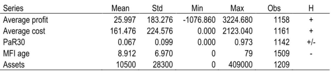
Table 3: Descriptive statistics of variables entering the analysis and their hypotheses
Series Mean Std Min Max Obs H
Average profit 25.997 183.276 -1076.860 3224.680 1158 +
Average cost 161.476 224.576 0.000 2123.040 1161 +
PaR30 0.067 0.099 0.000 0.973 1142 +/-
MFI age 8.912 6.970 0 79 1509 -
Assets 10500 28300 0 409000 1209
For definitions of variables, see table 2. “H” stands for the hypothesis in the analysis. A + sign means that the variable is supposed to be positively associated with the average loan size.
Assets are divided by USD 1,000.
29
Table 4: Correlation coefficients among the explanatory variables based on their case averages
Profit Cost Risk Age
Cost 0.4961
Risk -0.133 0.102
Age 0.0075 -0.052 0.1931
Size 0.1225 0.1375 0.029 0.1325
Raised number: The two-sided Pearson correlation coefficient is significant at the number’s level. For instance, the correlation 0.4961 is significant at the 1% level.
All monetary values are adjusted by the purchasing power parity GDP per capita obtained from IMF. “Profit” and “Cost” are averages per credit client. “Risk” is the PaR30 risk measure and “Size” is the MFI's assets.
30
Table 5: Are average profit, cost, and risk related to the MFI's average loan size?
Fixed effects Random First
Unstandardized Standardized effects difference
Constant -0.133 Average profit 3.032* 0.537* 5.756** 1.180 Average cost 3.870** 0.851** 4.050** 2.826*** PaR30 2.733 0.269 0.554 0.783 MFI age 0.021 0.147 0.009 0.040*** Assets 0.001 0.010 -0.001 0.001
Wald (F) test sign. 0.000 0.000 0.000 0.000
Hansen J test 0.771 0.771 0.936 0.802
N (Firm years) 741 741 741 736
The average loan size in rated microfinance institutions (MFI) regressed on profit function variables, risk, and control variables using different panel data methods. Data are from 1998 to 2008. The estimation is undertaken with the generalized method of moments (GMM) methodology using an optimal weighting matrix and robust standard errors (Woolridge, 2002). In the standardized regression the variables have zero average and standard deviation equal to 1.0.
Average loan is defined as the total value of outstanding loans divided by the number of credit clients. Average profit is the net annual result divided by the number of credit clients. Average cost is the total operating costs divided by the number of credit clients. PaR30 is portfolio at risk, that is, loans that are 30 days or more overdue as a fraction of total loans. MFI age is the number of years of microfinance experience. Assets are the total assets at the end of the year. All monetary variables are GDP per capita PPP adjusted with numbers from IMF, using the developing countries average GDP-PPP per capita as a benchmark. Average loan includes MFIs with average loans less than USD 10,000 (PPP-adjusted).
The instruments include the country variables GDP per capita (GDP-PPP adjusted), GDP growth, inflation, the current account balance as a per cent of GDP, and an economic freedom index from the Heritage Foundation. Furthermore, the one period lagged explanatory variables are also instruments.
A raised * means that the coefficient is significant at the 10% level; ** means significance at the 5% level, and *** means 1% significance level.
The Wald F test is an exclusion test of the hypothesis that all coefficients together are equal to zero (Greene, 2003 p. 107). A low significance value rejects the hypothesis. The Hansen (1982) J test is a test that the instruments are independent of the error term in the regression. A low significance level rejects independence.
31
Tab le 6: Are the MFI's lending methodology, its main market, and its gender bias related to average profit, cost, risk, the MFI's age, and its size?
Lending Main Gender
methodology Market bias
Average profits 0.002** 0.000 -0.001 Average costs 0.004*** 0.001*** -0.004*** Risk 4.513*** 0.089 -2.181*** MFI age 0.024* -0.025*** 0.006 Assets 0.000* 0.000 0.000*** Pseudo 𝑅2 0.153 0.095 0.095 LR test (sign.) 0.000 0.000 0.000 Observations 1015 1033 1040
Lending methodology is 1 if lending is mainly to individual, zero otherwise. Main market is 1 if lending is mainly to urban customers, 0 otherwise. Gender bias is 1 if the MFI has an explicit policy to target female customers.
Maximum likelihood estimation with logistic specifications on pooled data 1998 to 2008. Regressions include the country specific variables GDP per capita (GDP-PPP adjusted), GDP growth, inflation, the current account balance as a per cent of GDP, an economic freedom index from the Heritage Foundation; and year indicator variables.
A raised * means that the coefficient is significant at the 10% level; ** means significance at the 5% level, and *** means 1% significance level.
The LR test is an exclusion test of the hypothesis that all coefficients together are equal to zero (Greene, 2003 p. 107). A low significance value rejects the hypothesis.