Noname manuscript No.
(will be inserted by the editor)
Quantile Regression with Group Lasso for Classification
H. Hashem · V. Vinciotti · R. Alhamzawi · K. Yu
Received: date / Accepted: date
Abstract Applications of regression models for binary response are very com-mon and models specific to these problems are widely used. Quantile regres-sion for binary response data has recently attracted attention and regularized quantile regression methods have been proposed for high dimensional prob-lems. When the predictors have a natural group structure, such as in the case of categorical predictors converted into dummy variables, then a group lasso penalty is used in regularized methods. In this paper, we present a Bayesian Gibbs sampling procedure to estimate the parameters of a binary quantile regression model under a group lasso penalty. Simulated and real data show a good performance of the proposed method in comparison to mean-based approaches and to quantile-based approaches which do not exploit the group structure of the predictors.
Keywords quantile regression· binary regression· regularized regression· Gibbs sampling.
Mathematics Subject Classification (2000) 62H12·62F15 H. Hashem
Department of Mathematics, Brunel University London, UK
V.Vinciotti
Department of Mathematics, Brunel University London, UK Tel.: +44 (0) 1895267469
E-mail: [email protected]
R. Alhamzawi
College of Arts, University of Al-Qadisiyah, Iraq
K. Yu
1 Introduction
Quantile regression was introduced by Koenker and Bassett (1978) and has since then become the method of choice for regression problems where the data do not satisfy the normal distributional assumptions underlying tradi-tional methods or when the data are subject to some form of contamination. One line of research has extended the original quantile regression model to the case where the response is binary, as an alternative to traditional mean-based models, such as logistic and probit regression models. The methods were orig-inally developed in the frequentist estimation setting by Manski (1975, 1985) and were subsequently extended also to the Bayesian counterpart (Yu and Moyeed 2001; Benoit and Poel 2012; Migu´eis et al 2012) as a means to avoid large-sample based asymptotic results for inference and at the same time take regression parameter uncertainty into account.
In recent years, with the advent of highly dimensional and complex datasets in many application areas, regularized regression methods have attracted a lot of attention. These methods impose a penalty on the size of the parameters, thus making it possible to estimate regression coefficients in the presence of a large number of variables and a relatively small number of observations. In the popular lasso regression model, this penalty takes the form of an L1 penalty,
which has the advantage of providing simultaneous parameter estimation and variable selection (Tibshirani 1996). The original lasso method was extended in a number of directions, amongst which adaptive lasso (Zou 2006; Alhamzawi et al 2012) and Cox regularized regression (Tibshirani 1997). In some cases, the predictors have a natural group structure, such as in the case of a categorial variable being converted into dummy variables. In these cases, the selection of groups of variables is of interest, rather than of individual variables. In order to address this type of problems, Yuan and Lin (2006) developed the group lasso method and a number of authors have subsequently extended it and studied its theoretical properties (Bach 2008; Huang and Zhang 2010; Wei and Huang 2010; Lounici et al 2011; Sharma et al 2013; Simon et al 2013). Given the merits of the regularized methods just described, regularized methods for binary response variables have also been developed. In particular, Bae and Mallick (2004); Genkin et al (2007); Gramacy and Polson (2012) developed Bayesian logistic regression models under a lasso or ridge penalty, Meier et al (2008) developed the classical logistic regression model under a group lasso penalty, and Krishnapuram et al (2005) developed a sparse multinomial logistic regression model.
The references above refer to the estimation of mean-based regression mod-els. A small line of research has explored the link between the robust quantile regression models and the regularized models for high-dimensional data. In particular, Li and Zhu (2008) have developed quantile regression models un-der a lasso penalty, the theoretical properties of which are un-derived in Belloni and Chernozhukov (2011). Li et al (2010) provide a Bayesian formulation of the same problem. Finally, Ji et al (2012) have developed a quantile regression model under anL1penalty and for a binary response. In this paper, we extend
the work of Ji et al (2012) on binary quantile regression models with the use of a group lasso penalty. Our model is derived in the framework of probit binary regression and offers an alternative to the mean-based logistic regression model with group lasso penalty (Meier et al 2008), when the response is binary, the predictors have a natural group structure and quantile estimation is of inter-est. In section 2 we describe the model, in section 3 we describe the estimation of the parameters in a Bayesian setting, in section 4 we discuss how the model is used for prediction, in sections 5 and 6 we compare the performance of the method with related mean-based and quantile-based regression approaches on simulated and real data. Finally, in section 7, we draw some conclusions.
2 Binary quantile group lasso
Similar to a probit regression model, binary quantile regression models can be viewed as linear quantile regression models with a latent continuous response variables, e.g. Ji et al (2012). In particular, lety be the binary response vari-able, taking values 0 and 1, let xbe the vector of ppredictors, β the vector of unknown regression coefficients and (xi, yi), i = 1, . . . , n a sample of n observations on X and Y. Given a quantile θ, 0 < θ < 1, we consider the model:
yi⋆=xTiβθ+ui, i= 1, . . . , n and yi=h(yi⋆),
whereui are the errors, satisfyingP(ui≤0|xi) =θ, and his a link function. For binary response data, the link function is given byh(y⋆) =I(y⋆>0), with Ithe indicator function. In real applications,yis the observed binary response and the interest is to predictyfrom knowledge ofx.y⋆is unobserved and used mainly for modelling purposes. Some examples ofy⋆ include the actual birth weight of babies in a study where the aim is to investigate the factors behind the birth of premature babies, the credit risk of a customer in a study where the aim is to discriminate between good and bad customers (Kordas 2002) or the willingness to participate to work in a study where the factors behind the decision to work or not are investigated (Kordas 2006).
The attractive property of this latent model is that there is a correspon-dence between the quantiles ofy and the quantiles of y⋆, which are directly modelled. In particular, using the equivariance properties of quantile functions (Kordas 2006), it holds that
Qy|x(θ) =Qh(y⋆|x)(θ) =h(Qy⋆|x(θ)),
withQy|x(θ) denoting theθconditional quantile ofygivenx. From this, since Qy⋆|x(θ) =xTβθ under a linear quantile regression model, it follows that
Qy|x(θ) =h(xTβθ) =I(xTβθ>0).
So the estimation of the parameters βθ leads to the knowledge about the θ quantile of y. In the next section, we describe how to estimate βθ under a group lasso penalty.
3 Bayesian parameter estimation
In a binary quantile regression model, the parameterβθ is found by the fol-lowing minimization problem (Manski 1985):
min ||β||=1 n ∑ i=1 ρθ(yi−h(xTiβ)), (1)
whereρθ is the check function defined by ρθ(t) = { θt ift≥0, −(1−θt) ift≤0 or equivalentlyρθ(t) = |t|+ (2θ−1)t
2 . The restriction on||β||= 1 is motivated by the fact that the scale of the parameter is not identifiable, being y⋆ a latent variable. Yu and Moyeed (2001) have shown how minimizing (1) is equivalent to maximising the likelihood function, under the assumption that the error comes from an asymmetric Laplace distribution with density given by fθ(u) = θ(1 −θ) exp(−ρθ(u)). That is, minimising (1) is equivalent to maximising the likelihood
f(y|x, β, θ) =θn(1−θ)nexp ( − n ∑ i=1 ρθ(yi−h(xTiβ)) ) . (2)
This fact has created a straightforward working model for Bayesian inference quantile regression.
When the predictors have a natural group structure, the methodology above can be extended to the use of a group lasso penalty. In particular, sup-pose that the predictors are grouped intoGgroups andβg is the vector of co-efficients of thegthgroup of predictors. We denote withxigtheithobservation of the predictors in groupg. Letβ = (βT1, . . . , βGT)
T andxi = (xT i1, . . . , x
T iG)
T, i= 1, . . . , n. Under a group lasso constraint, the minimization in (1) becomes
min ||β||=1 n ∑ i=1 ρθ(yi−h(xTiβ)) +λ G ∑ g=1 ||βg||Hg, (3) where λ is a non-negative regularization parameter, controlling the sparsity of the solution, and ||βg||Hg = (β
T
gHgβg)1/2 with Hg = dgIdg and dg the dimension of the vector βg. The choice of dg in Hg has been suggested by Yuan and Lin (2006) to ensure that the penalty term is of the order of the variables in the group. Under an appropriate choice of prior distribution, the minimization problem in (3) can be shown to be equivalent to a maximum a posteriori solution. In particular, a Laplace prior onβg is chosen, that is
π(βg|λ) =Cdg √
det(Hg)λdgexp(−λ||βg||
whereCdg = 2−(dg+1)/2(2π)−(dg−1)/2/Γ((dg+ 1)/2) andΓ is the gamma func-tion. Then, using the same asymmetric Laplace distribution for the residuals u, the minimization in (3) is equivalent to the maximum of the posterior dis-tribution f(β|y, x, λ, θ)∝exp ( − n ∑ i=1 ρθ(yi−h(xTiβ))−λ G ∑ g=1 ||βg||Hg ) ,
under the constraint that||β||= 1.
3.1 Gibbs sampling procedure
We extend the Gibbs sampling procedure of Ji et al (2012) to the case of a group lasso penalty. As a first step we rewrite the prior ofβgusing the equality (Andrews and Mallows 1974)
a 2exp(−a|z|) = ∫ ∞ 0 1 √ 2πsexp (−z2 2s )a2 2 exp ( −a 2s ) ds,
which holds for anya ≥0. In particular, we take a=λ and z =||βg||Hg = (βT
gHgβg)1/2. Then the prior in (4) can be rewritten as
π(βg|λ) =Cdg √ det(Hg)λdgexp(−λ||βg|| Hg) (5) = (λ 2/2)(dg+1)/2 Γ((dg+ 1)/2) ∫ ∞ 0 exp ( −1 2β T g(sgH− 1 g )− 1βg)sdg2−1 g exp ( −λ2 2 sg ) √ det(2πsgHg−1) dsg.
As a second step, we use the fact that an asymmetric Laplace distributed random variable can be written as a mixture of aN(0,1) distributed random variable and an exponentially distributed random variable with rate parameter θ(1−θ) (Alhamzawi and Yu 2013; Kozumi and Kobayashi 2011; Lum and Gelfand 2012). This allows to rewrite the likelihood (2) as:
f(y|x, β, θ)∝exp ( − n ∑ i=1 ρθ(ui) ) = exp ( − n ∑ i=1 |ui|+ (2θ−1)ui 2 ) = n ∏ i=1 ∫ ∞ 0 1 √ 4πvi exp ( −(ui−ξvi)2 4vi −ζvi ) dvi withui=yi−h(xTiβ),ξ= (1−2θ) andζ=θ(1−θ).
From this, we can derive the following conditional distributions: f(β|y, x, λ, θ)∝ n ∏ i=1 ∫ ∞ 0 1 √ 4πvi exp ( −(ui−ξvi)2 4vi −ζvi ) dvi G ∏ g=1 exp ( −λ||βg||Hg ) f(β|y, x, v, λ, θ)∝exp ( − n ∑ i=1 (ui−ξvi)2 4vi − G ∑ g=1 λ||βg||Hg ) f(βg|y, x, v, β−g, λ, θ)∝exp ( − n ∑ i=1 (ui−ξvi)2 4vi −λ||βg||Hg ) .
If we write ˜yig =yi−h(∑Gk=1,k̸=gxTikβk)−ξvi, then using (5), we can write the conditional distribution ofβg as
f(βg|y, x, v, β−g, λ, θ)∝exp ( − n ∑ i=1 (˜yig−h(xTigβg))2 4vi −1 2β T g(sgHg−1)− 1β g ) . The derivations above lead to the following Gibbs sampling procedure for the quantileθ:
1. Sample y⋆from a truncated Normal distribution: yi⋆|yi, xi, β, vi∼ { N(xT iβ+ξvi,2vi)I(yi⋆>0) if yi= 1, N(xT iβ+ξvi,2vi)I(yi⋆<0) if yi= 0. 2. Samplevi−1, giveny⋆
i,xiandβ, from an inverse Gaussian distribution with mean and shape parameters given by, respectively,
µ= √ 1 (y⋆ i −x T iβ)2 and η= 1 2.
3. Sample sg, given βg and λ, from an inverse Gaussian distribution with mean and shape parameters given by, respectively,
µ= √ λ2 βT gHgβg and η=λ2. 4. Sample βg, giveny⋆, x, β
−g, sg, v, from a multivariate normal distribution
with mean and covariance given by
µg=ΣgxgV(y⋆−(1−2θ)v−xT−gβ−g) and Σg= (xgV xTg +s−
1
g Hg)−
1,
respectively, where V = diag
( 1
2vi )
, i = 1, . . . , n, and xg is the dg ×n matrix of observations for group g.
5. Sample λ2, given sg, from a Gamma distribution with shape and rate
parameters given by α=p+G 2 +b1 and β = G ∑ g=1 sg 2 +b2
respectively, withb1andb2two non-negative constants which we set equal
4 Class prediction
The estimation of the regression coefficients indicates the most influential vari-ables for the prediction of the binary outcome y. As with any classification problem, the main interest is in the prediction ofy from a new instancexfor which the binary outcome, or class, is unknown. In this section, we describe how the method that we propose is used to this purpose. The classification of an instance xis based on the estimated probability P(y = 1|x). For our model:
P(y= 1|x, β, θ) =P(y⋆>0|x, β, θ) =P(xTβθ+u >0|x, β, θ) =P(u >−xTβθ|x, β, θ) = 1−P(u <−xTβθ|x, β, θ) = 1−ΦALD(−xTβθ|x, β, θ),
whereΦALD is the cdf of an asymmetric Laplace distribution. Using the esti-matedβθ from the binary quantile regression model in the formula above, we get a natural estimate of the posterior probability of xbelonging to class 1. SinceP(u <0|x) =θ, it follows that (Kordas 2006):
xTβθ >=
< 0 ⇔ P(y= 1|x, β, θ) >
=
< 1−θ.
So there is a direct link before the estimated βθ and the probability that P(y = 1|x) = 1−θ. In general, we can expect the error to have a median around 0, which motivates the choice ofθ= 0.5.
In Kordas (2006), a second approach is also considered, whereP(y= 1|x, β) is computed as an average over different quantilesθ. In particular, it holds that
P(y= 1|x, β) = ∫ 1
0
I(xTβθ>0)dθ.
This probability can be estimated using a grid of values θ1, . . . , θmand then
taking P(y= 1|x, β)≈ 1 m m ∑ k=1 P(y= 1|x,βθˆk),
with ˆβθk the estimate ofβ for quantileθk.
As a final step in predicting y, we set a threshold t and classify a new objectxto class 1 if
P(y= 1|x)> t.
The thresholdt is normally chosen according to the relative misclassification costs for class 0 and 1 and corresponds to the caset= 0.5 for equal misclassi-fication costs (Hand and Vinciotti 2003).
5 Simulation study
In this section, we investigate the performance of our method with a simulation study. As typical for these applications, we simulate the data from
yi⋆=x T
iβθ+ui, i= 1, . . . , n and yi=h(y ⋆ i),
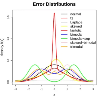
withβ chosen to have a group structure and with different choices of the error distribution. Similar to Yu et al (2013), we consider the following distributions for the error:
– Normal:N(0,1)
– t-distribution with 1 degree of freedom (Cauchy):t1 – Laplace distribution with location 0 and scale 10
– Skewed (skew): 15N ( −22 25,1 ) +15N ( − 49 125, ( 3 2 )2) +35N ( 29 250, ( 5 9 )2) – Kurtotic (kur): 2 3N(0,1) + 1 3N ( 0, ( 1 10 )2) – Bimodal (bim): 12 N ( −1, ( 2 3 )2) +12N ( 1, ( 2 3 )2) – Bimodal, with separate modes (bim-sep):12N
( −3 2, ( 1 2 )2) +12N ( 3 2, ( 1 2 )2) – Skewed Bimodal (skew-bim): 34N
( − 43 100,1 ) +14N ( 107 100, ( 1 3 )2) – Trimodal (tri): 209 N ( −6 5, ( 3 5 )2) +209 N ( 6 5, ( 3 5 )2) +101N ( 0, ( 1 4 )2) . These distributions were chosen to have a median close to or equal to zero. Figure 1 shows a plot of the density functions for the different cases considered. For the simulation, we set the sample size ton= 50.
For the β vector, we consider the case of a large number of predictors, i.e. p≫n. Similar to Li et al (2010), we create a group structure by simulating 10 groups, each consisting of 10 covariates. The 100 variables are assumed to follow a multivariate normal distributionN(0, Σ), with Σ having a diagonal block structure. Each block corresponds to one group and is defined by the matrixr|i−k|,i= 1, . . . ,10,k= 1, . . . ,10. For the correlationr, we experiment both withr= 0.95 (well-defined group structure) andr= 0.5. For theβvalues, we consider two cases:
1. The values for the first three groups are given by
(0.5,1,1.5,2,2.5,2,2,2,2,2),(2,2,1,1,1,1,3,3,3,3),(1,1,1,2,2,2,3,3,3,3) and they are set to zero for all other groups.
2. βj= 0.85 for allj.
We compare our method, Bayesian binary quantile regression with group Lasso penalty (BBQ.grplasso), with a frequentist mean-based logistic regres-sion model under a lasso penalty (R packageglmnet(Friedman et al 2010)), a frequentist mean-based logistic regression model under a group lasso penalty
−3 −2 −1 0 1 2 3 0.0 0.5 1.0 1.5
Error Distributions
x density f(x) normal t1 Laplace skewed kurtotic bimodal bimodal−sep skewed−bimodal trimodalFig. 1 Density functions of the errors considered in the simulation study.
(R packagegrpreg(Breheny and Huang 2014)) and a Bayesian binary quan-tile regression with a lasso penalty (R package bayesQR (Benoit and Poel 2012)). For grpreg and glmnet, the penalty parameter λ is selected using 5-fold cross-validation. For the Bayesian quantile methods and their Gibbs sampling procedures, we use 13000 iterations with the first 3000 iterations kept as burn-in. Furthermore, in the quantile methods, we use two methods to make class predictions, as described in Section 4: in the first case, we use the median (θ= 0.5); in the second case we take an average of three quantiles, which we set asθ= 0.25,0.5,0.75.
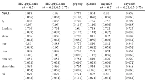
Tables 1 and 2 report the Area Under the Curve (AUC) values for the different methods and the different error distributions, with the AUC values averaged over 40 iterations and computed on a test set of the same size as the training set. In Table 1, we consider the first scenario for theβ values and we set r = 0.5, whereas in Table 2 we consider the case of all βs equal to 0.85 andr= 0.95. Similar results were obtained in the other cases. No significant differences were found between the two approaches for prediction used for the Bayesian methods, namely that based onθ= 0.5 and that based on the average of three quantiles. Tables 1 and 2 show how the BBQ.grplasso proposed in this paper significantly outperforms the other methods in all cases considered. Furthermore, the results show how grpreg is the worst performing method in all cases, surprisingly performing worse than glmnet, which is of a same nature but does not exploit the group structure of the predictors. The main competitor to BBQ.grplassoseems to be bayesQRwhich in fact differs with
Table 1 AUC values, averaged over 40 iterations (with standard deviations in brackets) for the case: n=50, p=100, r=0.5 andβvalues as in case (1).BBQ.grplasso: Bayesian binary quantile regression model proposed in this paper (based onθ= 0.5 (median) and an average of theθ= 0.25,0.5,0.75 quantiles);grpreg: frequentist mean-based logistic regression model with group lasso penalty,glmnet: frequentist mean-based logistic regression model under a group lasso penalty;bayesQR: Bayesian binary quantile regression with a lasso penalty (based onθ= 0.5 (median) and an average of theθ= 0.25,0.5,0.75 quantiles).
BBQ.grplasso BBQ.grplasso grpreg glmnet bayesQR bayesQR
(θ= 0.5) (θ= 0.25,0.5,0.75) (θ= 0.5) (θ= 0.25,0.5,0.75) N(0,1) 0.879 0.88 0.773 0.804 0.83 0.838 (0.055) (0.053) (0.103) (0.078) (0.066) (0.068) t1 0.838 0.838 0.725 0.765 0.787 0.797 (0.06) (0.06) (0.116) (0.116) (0.066) (0.068) Laplace 0.766 0.764 0.64 0.718 0.722 0.727 (0.089) (0.089) (0.125) (0.113) (0.087) (0.089) skew 0.885 0.886 0.792 0.811 0.832 0.837 (0.043) (0.043) (0.087) (0.086) (0.049) (0.051) kur 0.89 0.888 0.775 0.816 0.843 0.846 (0.049) (0.05) (0.112) (0.082) (0.058) (0.052) bim 0.898 0.898 0.782 0.789 0.853 0.857 (0.05) (0.05) (0.098) (0.117) (0.066) (0.065) bim-sep 0.881 0.881 0.784 0.819 0.826 0.829 (0.053) (0.053) (0.096) (0.078) (0.066) (0.072) skew-bim 0.885 0.886 0.797 0.814 0.838 0.848 (0.054) (0.055) (0.099) (0.09) (0.067) (0.066) tri 0.879 0.879 0.774 0.822 0.82 0.829 (0.053) (0.054) (0.117) (0.074) (0.064) (0.061)
the proposed method only in the use of the lasso penalty in contrast to the group lasso penalty. The tables also show how the superiority of the Bayesian methods version the frequentist methods is particularly pronounced for the case of non-sparse coefficients (Table 2). This is well known in the literature, as Bayesian regularized methods do not return exact zeros for the parameter estimates.
Figure 2 confirms the results of the tables by showing the average ROC curve of the methods considered for two cases of error distributions. The figures show how theBBQ.grplassooutperforms the frequentist mean-based methods for all classification thresholds and hasbayesQRas its main competitor.
6 Real application
In this section, we investigate the performance of the new method on five real applications:
– Birth weight dataset:This dataset is available in the R packagegrpreg and was used in Yuan and Lin (2006). The data record the birth weights of 189 babies, together with eight predictors. Among the predictors, two are continuous (mother’s age and weight) and six are categorical (mother’s race, smoking status during pregnancy, number of previous premature labours, history of hypertension, presence of uterine irritability, number
Table 2 AUC values, averaged over 40 iterations (with standard deviations in brackets) for the case: n=50, p=100, r=0.95 andβvalues as in case (2).BBQ.grplasso: Bayesian binary quantile regression model proposed in this paper (based onθ= 0.5 (median) and an average of theθ= 0.25,0.5,0.75 quantiles);grpreg: frequentist mean-based logistic regression model with group lasso penalty,glmnet: frequentist mean-based logistic regression model under a group lasso penalty;bayesQR: Bayesian binary quantile regression with a lasso penalty (based onθ= 0.5 (median) and an average of theθ= 0.25,0.5,0.75 quantiles).
BBQ.grplasso BBQ.grplasso grpreg glmnet bayesQR bayesQR
(θ= 0.5) (θ= 0.25,0.5,0.75) (θ= 0.5) (θ= 0.25,0.5,0.75) N(0,1) 0.962 0.962 0.606 0.895 0.928 0.943 (0.026) (0.027) (0.104) (0.046) (0.042) (0.046) t1 0.943 0.943 0.572 0.878 0.911 0.923 (0.033) (0.033) (0.096) (0.07) (0.048) (0.044) Laplace 0.872 0.872 0.57 0.784 0.834 0.848 (0.048) (0.048) (0.08) (0.1) (0.047) (0.047) skew 0.96 0.958 0.602 0.888 0.925 0.944 (0.025) (0.026) (0.104) (0.063) (0.038) (0.039) kur 0.954 0.955 0.646 0.876 0.917 0.941 (0.03) (0.031) (0.1) (0.087) (0.043) (0.037) bim 0.963 0.962 0.561 0.901 0.924 0.94 (0.033) (0.034) (0.086) (0.067) (0.045) (0.048) bim-sep 0.967 0.966 0.609 0.899 0.935 0.948 (0.029) (0.028) (0.119) (0.068) (0.036) (0.041) skew-bim 0.969 0.968 0.592 0.912 0.935 0.951 (0.019) (0.02) (0.107) (0.048) (0.033) (0.025) tri 0.96 0.959 0.601 0.89 0.928 0.94 (0.036) (0.036) (0.101) (0.071) (0.047) (0.042) t1 Error: r=0.5, case (1)
Average false positive rate
T rue positiv e r ate 0.0 0.2 0.4 0.6 0.8 1.0 0.0 0.2 0.4 0.6 0.8 1.0 BBQ.grplasso glmnet grpreg bayesQR
Laplace Error: r=0.95, case (2)
Average false positive rate
T rue positiv e r ate 0.0 0.2 0.4 0.6 0.8 1.0 0.0 0.2 0.4 0.6 0.8 1.0 BBQ.grplasso glmnet grpreg bayesQR
Fig. 2 Average ROC curves (over 40 iterations) of Bayesian binary quantile regression with
group lasso (BBQ.grplasso,θ= 0.5), compared withgrpreg,glmnetandbayesQR, under a
of physician visits). Through the use of orthogonal polynomials and dum-mmy variables, the data is converted into 17 predictors. The goal of this study is to identify the risk factors associated with giving birth to a low birth weight baby (defined as weighing less than 2500g).
– Colon dataset: This dataset is available in the R packagegglasso and was used by Yang and Zou (2013). The data report the expression level of 20 genes from 62 colon tissue samples, of which 40 are cancerous and 22 normal. In Yang and Zou (2013), the 20 expression profiles are expanded using 5 basis B-splines, creating a dataset with 100 predictors and a group structure.
– Labor force participation dataset: This dataset is available in the R package AER and was used by Liu et al (2013). The data come from the panel study of income dynamics in 1976 and contain 753 observations on women’s labour supply and 18 variables. The response variable, wife’s participation in work, is a binary variable and the predictors have a group structure, as defined in (Liu et al 2013). The aim of this analysis is to assess if there is a relation between several social factors (wife’s age, husband’s wage, wife’s father education etc.) and wife’s participation in work.
– Splice site detection dataset: This dataset is available in the R package grplassoand is a random sample of the data used in (Meier et al 2008). It contains information on 200 true human donor splice sites and 200 false splice sites. For each site, the data report the last three bases of the exon and the third to sixth bases of the intron. Thus, the data contain 7 cat-egorical predictors, with values A,C, G and T. These are converted into dummy variables, creating a natural group structure.
– Cleveland heart dataset: This dataset is available from the UCI machine learning repository. The data report information on 297 patients, 160 of whom have been diagnosed with heart disease and the remaining 137 have not been diagnosed with heart disease. The goal of the study is to predict heart disease from 13 predictors, related to patients’ characteristics (age, sex,etc) and clinical information (blood pressure, cholesterol level, etc). Four of the predictors are categorical and have been converted into dummy variables, creating a group structure.
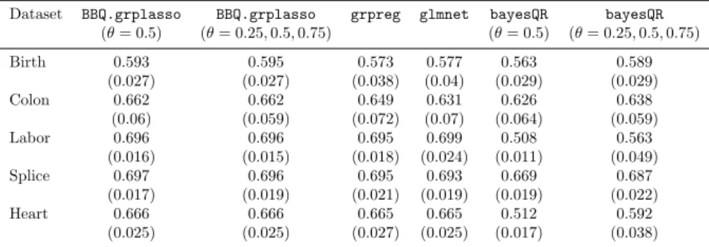
Table 3 reports the AUC values of 5-fold cross validation ROC curves, averaged over 30 iterations. As before, we compare the binary quantile re-gression method presented in this paper,BBQ.grplasso, withgrpreg,glmnet andBayesQR. The results show howBBQ.grplassois superior toBayesQRon all datasets, it outperforms the frequentist methods in the Birth and Colon datasets, but has comparable performances on the remaining datasets. Com-bined with the simulation study, this is probably a reflection of high levels of sparsity in the underlying model.
Table 3 AUC values, averaged over 30 iterations (with standard deviations in brackets) on the real data.BBQ.grplasso: Bayesian binary quantile regression model proposed in this pa-per (based onθ= 0.5 (median) and an average of theθ= 0.25,0.5,0.75 quantiles);grpreg: frequentist mean-based logistic regression model with group lasso penalty,glmnet: frequen-tist mean-based logistic regression model under a group lasso penalty;bayesQR: Bayesian binary quantile regression with a lasso penalty (based onθ= 0.5 (median) and an average of theθ= 0.25,0.5,0.75 quantiles).
Dataset BBQ.grplasso BBQ.grplasso grpreg glmnet bayesQR bayesQR
(θ= 0.5) (θ= 0.25,0.5,0.75) (θ= 0.5) (θ= 0.25,0.5,0.75) Birth 0.593 0.595 0.573 0.577 0.563 0.589 (0.027) (0.027) (0.038) (0.04) (0.029) (0.029) Colon 0.662 0.662 0.649 0.631 0.626 0.638 (0.06) (0.059) (0.072) (0.07) (0.064) (0.059) Labor 0.696 0.696 0.695 0.699 0.508 0.563 (0.016) (0.015) (0.018) (0.024) (0.011) (0.049) Splice 0.697 0.696 0.695 0.693 0.669 0.687 (0.017) (0.019) (0.021) (0.019) (0.019) (0.022) Heart 0.666 0.666 0.665 0.665 0.512 0.592 (0.025) (0.025) (0.027) (0.025) (0.017) (0.038) 7 Conclusion
In this paper, we present a novel method for binary regression problems where the predictors have a natural group structure, such as in the case of categor-ical variables. In contrast to existing methods for group-typed variables, we model the quantiles of the response variable, in order to account for possible departures from normality in the latent variable. In particular, we focus on class prediction and show how the probability of a new objectxbelonging to class 1, p(1|x), is directly linked to the quantile of the latent variable, since P(1|x) =P(y⋆>0|x). This motivates the use of quantile-based regression for probit regression models.
We compare our method with a frequentist mean-based logistic regres-sion model, under a lasso and a group lasso penalty, and with a Bayesian quantile-based regression model under a lasso penalty, on simulated and real data. The simulation shows a number of scenarios where the method out-performs the mean-based and quantile-based approaches. The R code of the method described in this paper is available fromhttp://people.brunel.ac. uk/~mastvvv/Software. Future research will consider an extension of this method to include a variable selection prior, similarly to the method of Al-hamzawi and Yu (2013) for Bayesian quantile regression.
References
Alhamzawi R, Yu K (2013) Conjugate priors and variable selection for bayesian quantile regression. Computational Statistics and Data Analysis 64:209–219
Alhamzawi R, Yu K, Benoit D (2012) Bayesian adaptive lasso quantile regression. Statistical Modelling 12(3):279 – 297
Andrews DF, Mallows CL (1974) Scale mixtures of normal distributions. Journal of the Royal Statistical Society, Series B 36:99–102
Bach F (2008) Consistency of the group lasso and multiple kernel learning. Journal of Machine Learning Research 9:1179–1225
Bae K, Mallick B (2004) Gene selection using a two-level hierarchical bayesian model. Bioin-formatics 20(18):3423–3430
Belloni A, Chernozhukov V (2011) Post l1-penalized quantile regression in high-dimensional
sparse models. Annals of Statistics 39:82–130
Benoit D, Poel D (2012) Binary quantile regression: a bayesian approach based on the asymmetric laplace density. Journal of Applied Econometrics 27(7):1174–1188 Breheny P, Huang J (2014) Group descent algorithms for nonconvex penalized linear and
logistic regression models with grouped predictors. To appear
Friedman J, Hastie T, Tibshirani R (2010) Regularization paths for generalized linear models via coordinate descent. Journal of Statistical Software 31(1):1–22
Genkin A, Lewis DD, Madigan D (2007) Large-scale bayesian logistic regression for text categorization. Technometrics 49(14):291–304
Gramacy R, Polson N (2012) Simulation-based regularized logistic regression. Bayesian Analysis 7(3):503–770
Hand D, Vinciotti V (2003) Local versus global models for classification problems: fitting models where it matters. The American Statistician 57(2):124–131
Huang J, Zhang T (2010) The benefit of group sparsity. The Annals of Statistics 38(4):1978– 2004
Ji Y, Lin N, Zhang B (2012) Model selection in binary and tobit quantile regression using the gibbs sampler. Computational Statistics and Data Analysis 56(4):827 – 839 Koenker R, Bassett GW (1978) Regression quantiles. Economerrica 46:33–50
Kordas G (2002) Credit scoring using binary quantile regression. Statistics for Industry and Technology pp 125–137
Kordas G (2006) Smoothed binary regression quantiles. Journal of Applied Econometrics 21(3):387–407
Kozumi H, Kobayashi G (2011) Gibbs sampling methods for bayesian quantile regression. Journal of Statistical Computation and Simulation 81:1565–1578
Krishnapuram B, Carin L, Figueiredo MA, Hartemink AJ (2005) Sparse multinomial logistic regression: Fast algorithms and generalization bounds. IEEE Transactions on Pattern Analysis and Machine Intelligence 27:957–968
Li Q, Xi R, Lin N (2010) Bayesian regularized quantile regression. Bayesian Analysis 5:1–24 Li Y, Zhu J (2008) L1-norm quantile regressions. Journal of Computational and Graphical
Statistics 17:163–185
Liu X, Wang Z, Wu Y (2013) Group variable selection and estimation in the tobit censored response model. Computational Statistics and Data Analysis 60:80–89
Lounici K, Pontil M, Tsybakov A, van de Geer S (2011) Oracle inequalities and optimal inference under group sparsity. Annals of Statistics 39:2164–2204
Lum K, Gelfand A (2012) Spatial quantile multiple regression using the asymmetric laplace process. Bayesian Analysis 7(2):235–258
Manski C (1975) Maximum score estimation of the stochastic utility model of choice. Journal of Econometrics 3(3):205–228
Manski C (1985) Semiparametric analysis of discrete response: asymptotic properties of the maximum score estimator. Journal of Econometrics 27(3):313–333
Meier L, van de Geer S, B¨uhlmann P (2008) The group lasso for logistic regression. Journal of the Royal Statistical Society, Serie B 70(1):53–71
Migu´eis LV, Benoit DF, Van den Poel D (2012) Enhanced decision support in credit scoring using bayesian binary quantile regression
Sharma D, Bondell H, Zhang H (2013) Consistent group identification and variable selec-tion in regression with correlated predictors. Journal of Computaselec-tional and Graphical Statistics 22(2):319–340
Simon N, Friedman J, Hastie T, Tibshirani R (2013) A sparse-group lasso. Journal of Com-putational and Graphical Statistics 22(2):231–245
Tibshirani R (1996) Regression shrinkage and selection via the lasso. Journal of the Royal Statistical Society, Series B 58:267–288
Tibshirani R (1997) The lasso method for variable selection in the cox model. Statistics in Medicine 16:385–395
Wei F, Huang J (2010) Consistent group selection in high-dimensional linear regression. Statistics in Medicine 16:1369–1384
Yang Y, Zou H (2013) A fast unified algorithm for solving group-lasso penalized learning problems
Yu K, Moyeed R (2001) Bayesian quantile regression. Statistics & Probability Letters 54:437– 447
Yu K, Cathy C, Reed C, Dunson D (2013) Bayesian variable selection in quantile regression. Statistics and Its Interface 6:261–274
Yuan M, Lin Y (2006) Model selection and estimation in regression with grouped variables. Journal of the Royal Statistical Society, Series B 68:49–67
Zou H (2006) The adaptive lasso and its oracle properties. Journal of the American Statis-tical Association 101:1418–1429