ALMA MATER STUDIORUM – UNIVERSIT `
A DI BOLOGNA
CAMPUS DI CESENA
Scuola di Ingegneria e Architettura
Corso di Laurea Magistrale in Ingegneria e Scienze Informatiche
Style Transfer with
Generative Adversarial Networks
Elaborato in
Machine Learning
Relatore
Prof. Davide Maltoni
Presentata da
Gabriele Graffieti
Seconda Sessione di Laurea
Anno Accademico 2017 – 2018
Abstract
In recent years, substantial advancements in machine learning have led us in the so-calleddeep learning revolution [1]. Tasks that were considered impossi-ble to be done by machines are now the foundation of many intelligent objects that surround us. This revolution has been possible thanks to the increasing complexity of learning models, which have been developed to resolve many different tasks, from object detection to automatic translation.
One of the most fascinating models isgenerative adversarial network (GAN), proposed by Goodfellow et al. in 2014 [2]. This model, as its name suggests, is able to generate new data that closely resemble the examples used dur-ing traindur-ing. The development of GANs has made possible one of the most challenging problems in computer vision: image-to-image translation. Just as language translation seeks to translate one sentence from one language to an-other without altering the meaning, image-to-image translation aims to map an image from one domain to another, without losing information about the content. As an example, a photograph taken at night can be translated to day conditions, even if a real image of the same scene during daytime does not exist.
Another task where GANs have demonstrated their potential is style transfer. Style transfer is the ability to merge two images together, keeping the content of the first picture applying the style of the second. Style transfer is nowadays mainly used for creating works of art, hence GANs are not only used by com-puter scientist, but also adopted by artists. For this reason, GANs used for artistic purposes are often renamed creative adversarial networks (CAN) [3]. This dissertation is focused on trying to use concepts from style transfer and image-to-image translation, not only to create art, but also to address some open problems in computer vision. In particular, the focus of experiments is concentrated on defogging. Defogging (or dehazing) is the ability to remove fog from an image, restoring it as if the photograph was taken during optimal weather conditions. The task of defogging is of particular interest in many
fields, such as surveillance or self driving cars.
In this thesis an unpaired approach to defogging is adopted, trying to trans-late a foggy image to the correspondent clear picture without having pairs of foggy and ground truth haze-free images during training. This approach is particularly significant, due to the difficult of gathering an image collection of exactly the same scenes with and without fog.
Many of the models and techniques used in this dissertation already existed in literature, but they are extremely difficult to train, and often it is highly problematic to obtain the desired behavior. Our contribute was a systematic implementative and experimental activity, conducted with the aim of attaining a comprehensive understanding of how these models work, and the role of datasets and training procedures in the final results. We also analyzed metrics and evaluation strategies, in order to seek to assess the quality of the presented model in the most correct and appropriate manner. In doing so, we focused on the aforementioned problem of defogging, trying to utilize the knowledge we have acquired to address a challenging research problem.
First, the feasibility of an unpaired approach to defogging was analyzed, using the cycleGAN model [4]. Then, the base model was enhanced with a cycle perceptual loss, inspired by style transfer techniques. Next, the role of the training set was investigated, showing that improving the quality of data is at least as important as the utilization of more powerful models. Finally, our approach is compared with state-of-the art defogging methods, showing that the quality of our results is in line with preexisting approaches, even if our model was trained using unpaired data.
Sommario (Italiano)
Negli ultimi anni, enormi avanzamenti nel campo dell’intelligenza artificiale, e in modo pi`u specifico nel machine learning, ci hanno proiettato nella cosiddetta
rivoluzione del deep learning [1], dove problemi che sembravano impossibili da risolvere in modo automatico, sono ora la base di molti degli oggetti intelligenti che ci circondano. Questa rivoluzione `e stata possibile grazie alla complessit`a sempre maggiore dei modelli di apprendimento automatico, i quali sono stati sviluppati per risolvere compiti molto diversi, come il riconoscimento di oggetti o la traduzione automatica.
Uno dei modelli pi`u interessanti `e detto generative adversarial network (rete avversaria generativa, GAN) ed `e stato proposto da Ian Goodfellow et al.
nel 2014 [2]. Tale modello, come il nome suggerisce, ha la propriet`a di poter generare nuovi dati, i quali sono indistinguibili dagli esempi usati durante il suo addestramento. GANs hanno reso possibile la soluzione di uno dei problemi pi`u impegnativi nell’ambito della computer vision, ovvero la traduzione di un’immagine in un’altra. Allo stesso modo della traduzione tra due linguaggi, che cerca di tradurre una frase da un linguaggio ad un’altro senza alterarne il significato, la traduzione tra immagini cerca di mappare un’immagine da un certo dominio ad un’altro, senza perdere informazioni sul contenuto. Ad esempio, `e possibile tradurre una fotografia scattata di notte, come se fosse stata scattata di giorno, anche se non esiste alcuna immagine della scena ripresa durante il giorno.
Un altro problema in cui i modelli avversari generativi hanno mostrato tutto il loro potenziale `e lostyle transfer. Esso consiste nel creare una nuova immagine, non esistente, che mantiene il contenuto di una certa immagine, e lo stile di un’altra. Oggigiorno lo style transfer `e sopratutto usato per creare nuove forme d’arte, e per tale motivo, le reti GAN non sono utilizzate soltanto da informatici, ma anche da artisti. Per tale motivo, i modelli GAN usati per scopi artistici sono spesso chiamatireti avversarie creative(creative adversarial networks, CAN) [3].
L’elaborato si focalizza nel cercare di utilizzare concetti derivati dallo style transfer e dalla traduzione tra immagini, non solo per creare arte, ma per risolvere alcuni problemi tutt’ora aperti in computer vision. Da un punto di vista pratico, il problema sul quale `e stato deciso di focalizzare l’attenzione `e quello della rimozione della nebbia da immagini (defogging). Tale problema `e di cruciale importanza in molte applicazioni pratiche, come la videosorveglianza o la guida autonoma.
Nel risolvere tale problema, `e stato adottato un approccio non accoppiato, dove un’immagine annebbiata viene tradotta nella corrispondente immagine in assenza di nebbia, senza avere coppie di immagini della stessa scena con e senza nebbia durante l’addestramento del modello. Questo approccio `e parti-colarmente significativo per il problema del defogging, poich´e `e estremamente complesso raccogliere un insieme di immagini della stessa esatta scena, con e senza nebbia.
Molti dei modelli utilizzati in questa tesi sono gi`a noti in letteratura, tuttavia essi sono estremamente complessi da addestrare, e spesso `e altamente prob-lematico ottenere il comportamento desiderato. Il contributo di questa tesi di Laurea `e una sistematica attivit`a implementativa e sperimentale, atta ad ottenere una profonda conoscenza di come tali modelli funzionano, e il ruolo del dataset e della procedura di addestramento nel risultato finale. Oltre a ci`o, diverse metriche sono state esaminate, in modo da valutare la qualit`a del nos-tro modello nel modo migliore e pi`u corretto possibile. Facendo ci`o, il focus `e caduto sul gi`a menzionato problema del defogging, scelto in modo da applicare le conoscenze acquisite in uno stimolante problema di ricerca.
Prima di tutto `e stato analizzata la fattibilit`a di un approccio non accoppiato, utilizzando un modello denominato cycleGAN [4]. In seguito, tale prototipo `e stato migliorato, attraverso una cycle perceptual loss, ispirata da diverse tecniche di style transfer. Dopo di che, `e stato investigato il ruolo del dataset di addestramento del modello, mostrando come l’utilizzo di immagini migliori sia importante quanto l’uso di modelli pi`u complessi. Infine, il modello risultate `e stato confrontato con lo stato dell’arte, mostrando una forte competitivit`a del nostro approccio, anche se esso `e stato addestrato con dati disaccoppiati.
Acknowledgments
First of all I would like to thank my parents, for considering my education and my happiness the most important thing in their lives. Thank you for investing most of your time, energy and money in order to make me able to follow my dreams. I hope to be worthy of all your sacrifices. In particular, I want to praise my father, for instilling me the germ of curiosity when I was a child. Wherever you are, I know you are proud of me.
I would also thank my second family, which is composed of my dearest friends Alfredo, Luca and Manuel, for making me smile during difficult periods, and for the wonderful moments we passed together.
This thesis would not have been possible without the constant support of my supervisor, prof. Davide Maltoni, who guide me through the entire process of the dissertation development, answering innumerable questions, discussing ideas and useful insights, and introducing me into the huge field of machine learning.
Lastly, I would like to thank all the people who freely share their knowledge over the Internet, allowing me to spend many pleasant evenings enriching my mind.
Contents
Abstract v
Sommario (Italiano) vii
Acknowledgments ix
Introduction 1
1 Background 3
1.1 Machine Learning . . . 3
1.1.1 Machine learning tasks and applications . . . 4
1.2 Computer Vision . . . 7
1.2.1 Typical tasks . . . 7
1.3 Artificial Neural Networks . . . 8
1.3.1 Artificial Neurons . . . 8
1.3.2 Multilayer Perceptron . . . 11
1.3.3 Loss Function . . . 13
1.3.4 The Backpropagation Algorithm . . . 15
1.3.5 Optimization tricks . . . 20
1.4 Deep Learning . . . 20
1.4.1 Regularization for deep learning . . . 21
1.5 Convolutional Neural Networks . . . 24
1.5.1 Building blocks . . . 25
1.5.2 Architecture . . . 26
1.5.3 Applications . . . 28
2 Generative Adversarial Networks 31 2.1 Generative Models . . . 31
2.1.1 Maximum likelihood estimation . . . 33
2.1.2 A taxonomy of generative models . . . 33
2.2 Adversarial networks . . . 35
2.2.1 Minimax games . . . 35
2.2.2 Model architecture . . . 36
2.3 Training . . . 37
2.3.1 Training algorithm . . . 38
2.3.2 Problems . . . 40
2.3.3 Possible solutions . . . 43
2.4 The problem of evaluation . . . 45
2.4.1 Why the loss function is not enough . . . 45
2.4.2 Assessment of result quality . . . 46
2.5 Examples and applications . . . 47
2.5.1 Examples . . . 47
2.5.2 Applications . . . 48
3 Cycle-Consistent Adversarial Networks 53 3.1 Image-to-image translation . . . 53
3.1.1 Style transfer . . . 54
3.1.2 Related work . . . 56
3.2 Cycle GAN . . . 58
3.2.1 The problem of paired data . . . 58
3.2.2 Cycle consistency . . . 59 3.2.3 General structure . . . 60 3.2.4 Details . . . 63 3.3 Training . . . 66 3.3.1 Training procedure . . . 67 3.3.2 Training improvements . . . 69 4 Experiments 71 4.1 PyTorch . . . 71 4.2 Defogging . . . 72 4.2.1 Related work . . . 74 4.3 Experiment design . . . 75 4.3.1 Dataset . . . 76 4.3.2 Metrics . . . 78 4.3.3 Set-up of experiments . . . 79
4.4 Getting started: cycle defogging . . . 80
4.5 Enhancing the model: cycle perceptual loss . . . 83
4.5.1 Cycle perceptual loss . . . 83
4.5.2 Evaluation . . . 85
4.6 The role of dataset . . . 88
4.7 Comparison with state-of-the-art methods . . . 92
4.7.1 Reference-based comparison . . . 92
CONTENTS xiii
5 Conclusions and future works 97
5.1 Conclusions . . . 97 5.2 Future works . . . 99
Introduction
What is a real image? How we can distinguish between a photograph or a computer generated picture? What are the essential features of what we call reality? These fairly philosophical questions have not been answered yet, though even a child can easily discern real and fake images. Before the advent of machine learning computers were programmed algorithmically: a procedure instructs the machine step-by-step, often in a deterministic and predetermined manner. However, not every aspect of our reasoning can be reduced to an algorithm, simply because we still do not know all the procedures involved. Nobody told us the exact algorithm to distinguish a cat from a dog, we simply have seen many cats and many dogs, and, during our infancy, other people told us which of them were cats, and which of them were dogs. We learned from data.
The same approach is the base of machine learning. Computers are not pro-grammed, but they learn directly from data how to perform their tasks. This paradigm is the foundation of many intelligent systems that nowadays surround us, from vocal assistants to self driving cars. However, unlike us, these models will be extremely confused if something unexpected is presented to them. As an example, if we present a photograph of a dog with wings to a classificator, probably the output class will be dog, or bird, because the model cannot use its knowledge to create new classes. Unlike us, machine learning models are not creative, they usually do not aggregate their knowledge to produce new items.
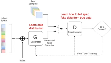
In 2014, Goodfellowet al. introduced generative adversarial networks (GAN) [2], a machine learning model that can generate new data similar to the exam-ples used during training. GANs learn the intrinsic features of the data and the data distribution, and, starting from a noise vector, they produce a totally new sample, which is indistinguishable from the real data. In order to perform well, GANs have to correctly answer the questions reported at the beginning of this chapter. GANs, like us, learn, somehow, the difference between real and fake data, and use this knowledge to produce realistic samples.
In the last few years, GANs have been enhanced in order to carry out increas-ingly complex tasks, such as style transfer and image-to-image translation. Style transfer is the ability to mimic the style of an image, keeping unchanged the content of the original picture. Given a photograph, machine learning models can apply the style of a portrait, producing works of art that never existed before. Computers have become creative.
Image-to-image translation is an even more complex task than style transfer. Images are translated from one domain to another, such as from summer to winter, or from day to night. A particular model derived from GAN and named cycleGAN [4] has shown impressive results in image-to-image translation, using an unpaired approach. The model is trained with two collections of images, representing the two domains that have to be translated. CycleGAN learns the most important features that distinguish the two domains, and it finds out a mapping directly from data, with the aim of correctly generating an image in one domain, given a photograph in the other.
The full potential of these creative models has not yet been explored; thus, the aim of this dissertation is to deeply understand these approaches and tech-niques, and apply them to an open research problem: removing fog from im-ages. In chapter 1 a brief background about machine learning and neural networks will be covered. In chapter 2 and chapter 3 generative adversar-ial networks and cycleGAN are examined in details, with a particular focus on the learning procedure. In chapter 4 results of experiments on defogging are reported, and compared with the state-of-the-arts methods. Finally, in chapter 5, conclusions will be drawn, and future work directions suggested.
1
Background
Science is like a hungry furnace that must be fed logs from the forest of ignorance that surrounds us. In the process, the clearing we call knowledge expands, but the more it expands, the longer its perimeter and the more ignorance come to view.
– Matt Ridley, Genome (1999) In this chapter a brief introduction to machine learning is provided. The goal of the following sections is to introduce the reader to the principal topics and techniques of machine learning, and present the recent developments in the field.
1.1
Machine Learning
Learning is commonly described as the acquisition or modification of knowledge and behaviors, as a result of interaction with the environment. This ability is possessed even by the simplest of animals and by some plants [5]. Learning can be achieved through education, experience, training or the processing of acquired data, in order for it to be organized it more generally or to infer new knowledge.
How learning works has been a mystery for a long time, and only in the last cen-tury, with the development of psychology, cognitive science and neuroscience, have some of the processes involved in learning come to light.
Since the advent of computers, producing machines capable of learning in a human-like manner has been one of the most compelling task in computer
science, and a great example of multidisciplinary research. It has also led to the creation of completely new subjects, such as artificial intelligence or
computational neuroscience. The study of computational modeling of learning constitutes the foundation of machine learning.
Since the dawn of artificial intelligent research, many problems marked as difficult to solve by humans have been solved by machines, especially in the field of optimization. Surprisingly, many problems which are easy to solve by people, such as classifying or detecting objects in an image, proved to be extremely difficult for computers to achieve. This phenomenon can be explained by the lack of formalism for the aforementioned problems. In fact, it is nearly impossible to produce a classical algorithm that can detect components in an image when executed by a machine. One of the most effective way to produce such behavior is t train a computer in the same manner as children are instructed to recognize common object during their infancy.
Overall, machine learning can be described as a field of study aimed to give ma-chines the ability to learn from data, without being explicitly programmed. In this sense, learning is formalized by the famous statement by Tom M. Mitchell “A computer program is said to learn from experience E with respect to some class of tasks T and performance measure P, if its performance at tasks in T, as measured by P, improves with experience E” [6]. The importance of this definition is twofold: it describes machine learning in a formal way, and it emphasizes the role of performance evaluation.
1.1.1
Machine learning tasks and applications
The learning process of alearning model is commonly composed of two phases: thetraining phase, when the model actually learn from the given data, and the
evaluation phase, when the performance of the model is assessed. From the definitions given in section 1.1 emerges that machine learning relies heavily on data. Data can be arranged in any form, from numbers to sequences. Usually the data is organized in a dataset, which is often split in three independent collections [7]:
• Training set: contains the data used for training the model in the training phase.
• Test set: contains items not present in the trainig set (the model does not see the elements of the test set during training) and it is used for evaluating the performance after the training phase.
1.1. Machine Learning 5
• Validation set: contains data used for hyper-parameters validation and tuning.
Normally the training set contains a larger amount of data than the other two. A rule-of-thumb ratio of the sets dimensions is: 60% of the data go to the training set, and 20% to the test and validation set, respectively. However, if the number of samples is small, utilizing a subset of them for validation alone can cause unreliable estimations of the performance of the model. In these cases a common approach is to use cross validation [8].
Tasks
Historically, machine learning tasks are divided into three broad categories, based on the nature of the data, the presence of additional information, the nature of feedback given to the model and the nature of the task to accomplish [7].
• Supervised learning: in this approach the model infers a function fromsupervised orlabeled data. The training set consists of input-output pairs, and the goal of the model is to infer the correct mapping between the inputs and the outputs. The inferred function has to be general in order to yield the correct output from an unseen input.
• Unsupervised learning: the data do not contain any additional infor-mation, and the goal of the model is to learn how to analyze the data, in order to find patterns or structures. An unsupervised approach can be the goal of the model (e.g. in the case of clustering), or an intermediate data analysis step.
• Reinforcement learning: in this case the learning model interacts directly with the environment, and learns from the consequences of its actions. The data consists of information about the environment and the set of available actions. When an action is performed, the RL-agent receives a reward, which indicates how positive was the action’s outcome was. The goal of an RL-agent is to maximize the accumulated reward over time.
These categories are partially overlapped, i.e. between supervised and un-supervised learning lies the category of semi-supervised learning, where some (often many) of the entries in the training set are not labeled, or some labels are not correct.
years is active learning. In this approach, unlabeled data is abundant and labeling them is possible, but expensive in terms of time or resources. In this scenario, a learning model can actively query some external entity for the labels of a subset of data. The aim of the active learning agent is to analyze the data and seek the most suitable items that require labeling by the external entity, in order to infer the most general input-label map with the lowest amount of labeled data.
Applications
Another categorization of machine learning tasks arises when considering the desired output of the learning system [7]:
• Classification: the input is divided in two or more classes, and the goal of the learning-agent is to produce a model which assigns to an unseen input one or more of these classes. This is a typical application of super-vised learning, when the training data is labeled with the correspondent class.
• Regression: the output of the model has to be continuous rather than discrete (e.g. the weight of a person given her/his height). As well as classification, regression is mainly accomplished through supervised learning.
• Clustering: the input data has to be divided into groups. The groups are usually not known beforehand, making clustering a typical example of unsupervised learning.
• Density estimation: finds the distribution of input data in a defined space. The inferred distribution can be used for statistical analysis of the data, or for generating artificial data that closely resemble the real one.
• Dimensionality reduction: simplify the data, learning a representa-tion into a lower-dimensional space.
• Representation learning: in many machine learning models, raw data has to be pre-processed in order to extract significant features, which are provided as input to the model. Representation learning aims to learn how to automatically extract those features from raw data. Many of the machine learning models used nowadays use representation learning techniques to extract the necessary feature to solve the problem from raw data.
1.2. Computer Vision 7
1.2
Computer Vision
Computer vision is an interdisciplinary field that deals with how machines can be made to acquire high-level understanding from digital images or videos. It also seeks to automate tasks that the human visual system can do [9]. This image understanding can be seen as the disentangling of symbolic information from image data, using contributions from physics, biology, geometry, statistic and machine learning.
The representation of visual data can widely vary widely according to different applications, ranging from simple RGB images, sequences of images, views from multiple cameras or multi-dimensional data from a medical scanner. Since the majority of information that we process are acquired through the sight, it is a little surprise that many machine learning models are used for computer vision. Some of these models are directly related to their biological counterpart, such asconvolutional neural networks, which will be discussed in section 1.5.
1.2.1
Typical tasks
Computer vision is a wide and active research area, and for this reason is commonly divided into subfields. Some of the most important fields are:
• Recognition: the classical problem in computer vision. The goal is to determine whether or not the the image contains some specific object, such as a face.
• Motion analysis: a sequence of images is processed, in order to produce an estimate of the velocity at each point in the image. A typical example of motion analysis is tracking, where an object is followed throughout the image sequence.
• Scene reconstruction: given one or more images (or a video) of the same scene, the objective is to reconstruct the 3D model of the scene.
• Image restoration: the aim is the removal of noise from images. Noise can be caused by movement, blur, occlusions or atmospheric phenomena, such as fog or rain.
1.3
Artificial Neural Networks
In machine learning, artificial neural networks (ANNs) are computing systems inspired by thebiological neural networks that constitute the brains of animals [7]. Initially artificial neural networks were developed to solve problem in a general way, as the human brain does. However, over time, the attention shifted to more specific tasks, often departing from the initial biology-inspired systems [10]. Artificial neural networks have been used on a wide variety of tasks, from speech recognition to medical diagnosis.
ANNs are generally composed of interconnected units called neurons, which send signals to each other through their connections. Each connection has a numeric property, calledweight, that can be tuned during the training phase, making ANNs capable of learning from data. Following this reason an artificial neural network can be seen as the functionf :X →Y, which maps some input
x∈ X to some output y ∈ Y. f is characterized by learnable parameters θf,
which represent the weights of the connections.
1.3.1
Artificial Neurons
Neurons used in artificial neural networks were initially developed taking in-spiration from the biological neurons present in the brain of most animals. A neuron (or nerve cell) is a specialized cell that receives, processes and transmits information through electrical and chemical signals [11]. These signals between neurons occur via connections called synapses. Neurons can connect to each others to form neural circuits, or neural networks. Taking inspiration from biological neurons, Frank Rosenblatt developed the concept of the perceptron
[12]. A perceptron is a mathematical abstraction of a biological neuron and, at the same time, a binary classifier. As actual neurons, the perceptron can be fed with more than one input source. It receives an input vectorx consisting of n elements, and produces a single output y (see Figure 1.1). A perceptron is characterized by a set of n weights, one for each input, and a threshold. In the classical model, the output of the perceptron is binary, and is positive if the weighted sum of the inputs is greater than the threshold:
y= ( 0 if Pn i=1wixi ≤threshold 1 if Pn i=1wixi > threshold (1.1) The learnable parameters are the weights and the threshold. By varying them, different models of decision-making can be obtained, according to the problem. Making a parallel with a biological neuron, the input vectorxrepresents signals
1.3. Artificial Neural Networks 9
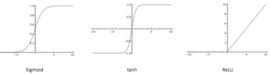
Figure 1.2: Some of the most used activation functions.
collected by the synapses of the neuron and the weights w represent the the modulation (e.g. amplification/attenuation) operated by each synapse to the corresponding input.
Figure 1.1: A percep-tron.
The perceptron is also a binary classifier: suppose that the inputs can be distinguished in two classes, a value of y equal to zero can represent the first class, and a value equal to one, the second class.
The classic perceptron model is the easiest one, and starting from it many more neural models were de-veloped using it as a starting point. The output of a classic perceptron is strictly binary, and this can be a disadvantage during learning. In fact, a small change in the weights or the threshold may switch the out-put of the neuron from zero to one or vice versa. In order to overcome this limitation, different activation functions were evolved. The most famous of these is the sigmoid function:
σ(z) = 1
1 +e−z. (1.2)
The sigmoid function is continuous, derivable, and its image vary from zero to one. This function is suitable during learning, because small changes in the perceptron’s parameters are reflected in small changes in the output. A per-ceptron which uses the sigmoid function is commonly called asigmoid neuron. Using a sigmoid function, the output of a neuron becomes:
y= 1
1 + exp(−Pn
i=0wixi−t)
. (1.3)
wheret is the threshold.
In some cases, the sigmoid function is replaced by the hyperbolic tangent (tanh or softmax), so the output of the neuron varies from -1 to +1.
Another widely used activation function is the rectifier (ReLU) [13]:
f(z) = z+=max(0, z). (1.4)
The rectifier, apart from being biologically inspired, has shown better perfor-mance during the learning phase, especially in deep networks [14], and for this reason, is the most used activation function for deep models [15]. A graphical representation of the most common activation function is shown in Figure 1.2.
Learning
As stated earlier, a perceptron, regardless of the activation function used, can be considered a simple binary classifier, and a learning strategy can be adopted to find the optimum combination of parameters. Given a binary labeled training set, the error of the perceptron can be expressed as:
E(w, t) = 1 2 m X j=1 f n X i=1 (wi·x (j) i )−t ! −l(j) !2 (1.5) where:
• w is a vector containing the weights of the perceptron.
• t is the threshold associated with the perceptron.
• m is the number of elements in the training set.
• f is the activation function.
• x(j) is thej-th element of the training set.
• l(j) is the desired result (label) associated with the j-th element of the
training set.
• n is the number of elements in the input vector x.
To simplify the notation, the thresholdt can be included in the weight vector (w0 =t) and associated with an input x0 = 1; thus Equation 1.5 becomes:
E(w) = 1 2 m X j=1 f n X i=0 (wi·x (j) i ) ! −l(j) !2 (1.6) Hence, the objective is to find the optimal combination of values of w which minimize the error. Let
Wx(j)(w) = f n X i=0 (wi·x (j) i ) ! −l(j) !2 (1.7)
1.3. Artificial Neural Networks 11 the error of the perceptron for the input vector x(j). An approach based on
gradient descent can be applied, in order to update w to minimize the error. The gradient of Wx(j)(w) (∇Wx(j)(w)) indicates the direction of maximum
growth of Wx(j)(w) with respect to w. The opposite direction (−∇Wx(j)(w)),
on the contrary, indicates the direction of faster decrease of the function, with regards to w. If the weights are updated following the opposite direction of the gradient, the function will be minimized. Using an iterative method, it is possible to get closer and closer to the minimum point, which correspond to the optimal solution of the optimization problem stated as:
s∗ = min w m X j=1 Wx(j)(w) (1.8)
The update of the weighs occurs with the following procedure:
wj+1 =wj−η∇Wx(j)(w) ∀j ∈ {1, . . . , m} (1.9)
where:
• wj is the vector of the weights at step j
• η is the learning rate, which is the displacement step used to update w. If it is too large, the optimum may be impossible to reach, whereas if it is too small, it can greatly slow down convergence. The learning rate is a typical example of a hyper-parameter.
Thanks to Equation 1.9, a perceptron can learn how to classify data simply by being exposed to the data itself. However, the perceptron can only solve binary classification problems, and the classification is linear, which means that it may not perform well if the patterns are not linearly separable.
In spite of that, the perceptron is the fundamental building block of most of the neural network models, currently used to solve many extremely complex tasks in the field of machine learning.
1.3.2
Multilayer Perceptron
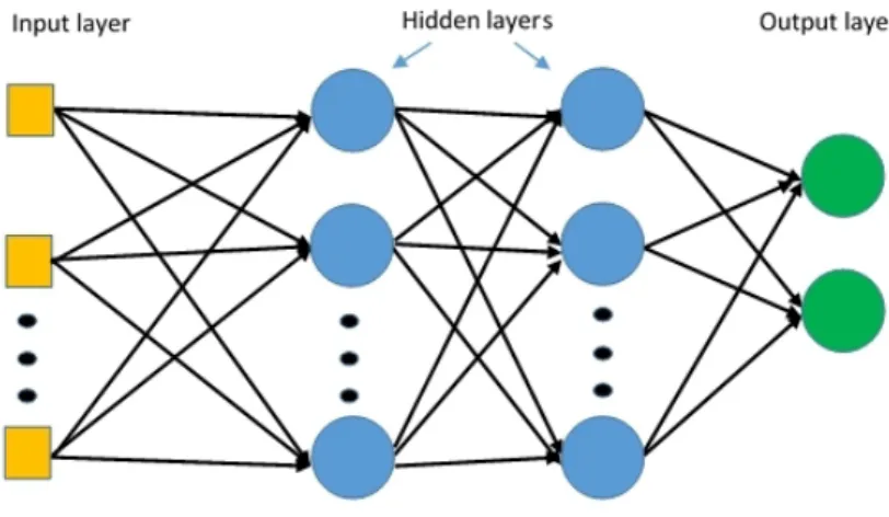
Following the biological inspiration that led to the development of artificial neurons, it seemed natural to try to connect them together, in order to form neural networks similar to those present in the brain, seemed natural. The first example of an artificial neural network was themultilayer perceptron(MLP). In a multilayer perceptron the neurons are organized in layers, and the outputs of the neurons of one layer are the input to the next layer. The minimum
number of layers is three, one input layer, one or more hidden layers and one output layer.
Figure 1.3: A multilayer perceptron with four layers.
A multilayer perceptron is an example of afeedforward neural network. These kinds of model can classify patterns in more than two classes, and separate them non-linearly. Moreover, a feedforward neural network with only one hidden layer and a finite number of neurons has been demonstrated to be a
universal approximator [16]. This means that a simple neural network can represents a wide variety of interesting functions, when given appropriate pa-rameters. This theoretical result is one of the reasons for the widespread adoption of neural networks for a wide range of different problems.
A multilayer perceptron usually has the following properties:
• In an MLP the number of input neurons should be equal to the number of dimensions of the input, i.e. if the input is a 3-dimensional vector, the network should have three neurons in the input layer.
• A MLP should have as many perceptrons in the output layer as the number of classes. The value produced by an output neuron represents the probability that the current input will be classified with the class associated to the neuron.
• A MLP should associate an input to the class represented by the output perceptron by computing the highest value among its peers.
• In a MLP all the neurons should have the same activation function.
• In a MLP every perceptron can only be connected to perceptrons in the next layer.
1.3. Artificial Neural Networks 13 Figure 1.3 shows a common example of MLP architecture, composed of two hidden layers. In the example, the MLP acts as a binary classifier (there are only two neurons in the output layer). The perceptrons in the input layers usually do not compute any function, but simple propagate the input to the first hidden layer.
Besides MLP, many other types of neural networks exist, which differ from each other in terms of their architecture and the organization of neurons. One model worth mentioning here is therecurrent neural network (RNN), in which cycles are present between units of neurons. RNNs have gained popularity in recent years as a result of their extensive use with time sequences.
1.3.3
Loss Function
In section 1.3.1 it is stated that, in order to be able to learn, a perceptron should take classification error into consideration, and try to minimize it. Equation 1.5 is an example of a loss function.
Generally, a loss function (or cost function) is a function that maps an event or values onto a real number, which represents a certain cost associated with the event. In many optimization problems, the goal is to minimize the cost function, or, in a parallel way, maximize the objective function (which is the negative of the cost function). A loss function is often used in statistics as a parameter estimation of a distribution, computing the difference between real and estimated data. In classification, a loss function is usually a penalty for an incorrect classification, and it grows in accordance with the classification error.
The choice of the most suitable loss function is a problem of crucial importance, and the differences in performance and accuracy of the same model trained with different loss functions may be broad.
Application of loss function is not limited to neural networks, on the contrary, it is a common concept in various machine learning models. The most commonly used loss functions are described below.
Squared loss
The squared loss (or mean square error) is formulated as:
L(Y,Yˆ) = 1 n n X i=1 (y(i)−yˆ(i))2. (1.10)
where:
• y(i) ∈Y are the observed data.
• yˆ(i) ∈Yˆ are the predictions of the model.
• n is the number of elements in the training set.
The target of the squared loss function is to minimize the residual sum of squares. This loss function suffers from slow convergence when used with neu-rons that use the sigmoid function. It also tends to penalize outliers excessively, and if there are many of them present in the training data, the convergence may be difficult. Hence, squared loss is more commonly used for regression tasks, rather than classification.
Mean absolute error
The mean absolute error, or L1 loss, is formulated as:
L(Y,Yˆ) = 1 n n X i=1 |y(i)−yˆ(i)|. (1.11) This loss is similar to squared loss, but it penalize outliers less, so it is preferred in this sense. However, the mean absolute loss has the same gradient for every point, regardless of the distance to the optimum, hence it is more difficult to find the optimal solution.
Cross entropy loss (log loss)
Cross entropy loss is commonly used in binary classifiers (labels are 0 or 1), and it is formulated as:
L(Y,Yˆ) = 1 n n X i=1 [−y(i)log(ˆy(i))−(1−y(i)) log(1−yˆ(i))]. (1.12) Cross entropy loss is closely related to the Kullback-Leibler divergence, which measures the difference between two distributions. If the cross entropy loss is large, its means that the distribution of real data is different from what has been predicted. Cross entropy loss is usually preferred to squared loss, especially in deep models, due to its faster convergence. Cross entropy loss can be generalized for multiclass problems, incategorical cross entropy [8].
1.3. Artificial Neural Networks 15
1.3.4
The Backpropagation Algorithm
section 1.3.1 describes how a single perceptron can learn the optimal set of parameters directly from data. Does a similar algorithm exists for training a neural network, potentially composed of milions of neurons? Ever since the 1960s, research had been carried out to provide possible answers to this ques-tion [17] and by 1970 the first version of the backpropagaques-tion algorithm was developed by Seppo Linnainmaa [18]. However, the algorithm remained mostly unknown, mainly due to the limited computing power of machines at the time. Backpropagation gained recognition after the publication by Rumelhartet al.
in 1986 [19].
The backpropagation algorithm is an optimization algorithm, which minimizes the loss function by changing the parameters of the model. Since its introduc-tion, the backpropagation algorithm has been thede factostandard for training neural networks, especially in recent years, when it benefits form cheap and powerful GPU-based computer systems.
The backpropagation algorithm repeats a two phases cycle: propagation and weight update. In the first phase, an input vector is propagated through the network, layer by layer, until it reaches the output layer. The output of the network is then compared to the desired output, using a derivable loss function. The resulting error is calculated for each neuron in the output layer, and then propagated from the output layer back to the input layer (as the name backpropagation suggests), until each neuron has an associated error value. After that, those errors are used to calculate the gradient of the loss function. In the second phase, the weights are modified by an optimization procedure, according to the gradient of the loss function.
Stochastic gradient descent
The backpropagation algorithm is an example of gradient descent optimization. The goal of the procedure is to find a minimum in a function, changing its parameters according to the opposite direction indicated by the gradient. Let F(·) be a continuous function defined by parameters θ. Let θn be the
parameters at iterationn. If we want to minimizeF(θ) using gradient descent, the parameters of the next step are updated as follows:
θn+1 =θn−η∇F(θn) (1.13)
In most machine learning models the function to be minimized is the loss function. As described in subsection 1.3.3, if the training set is composed of
m items, the loss function usually assumes the form: L(Q(X, θ), Y) = 1 m m X i=1 Li(Q(x(i), θ), y(i)). (1.14) where
• x(i)∈X is an element of the training set.
• y(i) ∈Y is the label associated to the i-th item of the training set.
• Q(X, θ) is the output of the neural network.
• Li(Q(x(i), θ), y(i)) is the per-example loss.
Updating the parameters of such a model with gradient descent requires com-puting: θn+1 =θn−η 1 m m X i=1 ∇θLi(Q(x(i), θ), y(i)). (1.15)
which has a computational cost ofO(m), thus computing the gradient can be prohibitive if the training set contains billions of examples.
In order to overcome the problem, the gradient can be computed using a small subset of samples, so that the optimization is based on an estimation of the gradient rather than the actual gradient. This approach is called stochastic gradient descent (SGD). The parameters are updated considering a set of m0
examples (minibatch), drawn uniformly from the training set. The number of sampled example is usually much smaller than the training set. The update to the parameters is performed as:
θn+1 =θn−η 1 m0 m0 X i=1 ∇θLi(Q(x(i), θ), y(i)). (1.16)
One notable case is when m0 = 1. In this particular case, the update to parameters is performed after every iteration.
SGD has made the training of models through gradient descent on very large datasets possible. Indeed, for a fixed model size, the cost per SDG update does not depend on the training set dimension. It can consequently be stated that the computational cost of one step of SGD is O(1), as a function of m
1.3. Artificial Neural Networks 17
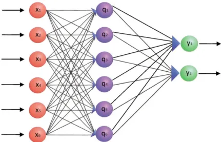
Figure 1.4: A multilayer perceptron
The algorithm
Consider the neural network displayed in Figure 1.4. Assuming that a mini-batch of dimension 1 is used, so for every iteration a new input is considered. Generalizing, the output of the hidden layer’s neutrons are q1, q2, . . . , qm and
can be computed as:
qi =f(vix) ∀i∈ {1, . . . , m} (1.17)
Then,y1, y2, . . . , yn are the output of the network, and can be computed as:
yi =f(wiq) ∀i∈ {1, . . . , n} (1.18)
where:
• wi is the weights vector associated with the i− th perceptron in the
output layer.
• viis the weights vector associated with thei−thperceptron in the hidden
layer.
• f is the activation function.
LetLx(y) be the loss on the current inputx. The loss can be seen as the error
made by the network when it is fed withx. It is possible to begin decomposing this error by calculating the error of the output layer’s neurons. This can be expressed as:
ei =
∂Lx(y)
∂yi
which represents how much the loss varies due to small changes inyi. Since the
only way to modifyyi is to change the weights wi or the hidden layer output
q, we can rewrite Equation 1.19 as:
ei =
∂Lx(y)
∂wiq ∀i∈ {1, . . . , n} (1.20)
which for the chain rule of calculus becomes:
ei = ∂Lx(y) ∂yi · ∂f(w iq) ∂wiq = ∂Lx(y) ∂yi f0(wiq) ∀i∈ {1, . . . , n} (1.21) Now we want to calculate the error of the hidden layer, which is equal to:
ri = ∂Lx(y) ∂qi · ∂f(v ix) ∂vix = ∂Lx(y) ∂qi f0(vix) ∀i∈ {1, . . . , m} (1.22) The first term of the equation can be rewritten, using the chain rule of calculus as: ∂Lx(y) ∂qi = n X j=1 ∂Lx(y) ∂yj · ∂f(w jq) ∂wjq · ∂wjq ∂qi = n X j=1 ej· ∂wjq ∂qi (1.23) And since ∂w∂qjq i =wi
j what is obtained is that:
ri =f0(vix) n
X
j=1
ejwij ∀i∈ {1, . . . , m} (1.24)
In case of a neural network with more than one hidden layer, the errors of the others layers are calculated by repeating Equation 1.24, treating the next hidden layer as if it were the output layer.
After the error backpropagation, the weights of the network are updated. Starting from the output layer, a small change in a weight produces the fol-lowing variation on the loss:
∂Lx(y) ∂wi = ∂Lx(y) ∂yi · ∂f(w iq) ∂wiq · ∂wiq ∂wi =ei·q ∀i= 1, . . . , n (1.25)
So the weights can be updated with the following criterion:
wi =wi+η·ei·q ∀i∈ {1, . . . , n} (1.26)
And, similarly, the weighs of the hidden layer can be adjusted as follow:
1.3. Artificial Neural Networks 19
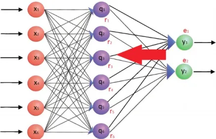
Figure 1.5: The error is back-propagated through the network, in order to update the weights accordingly.
At the end of the backpropagation operations, the weights of the network are updated in order to take a step towards the opposite direction of the gradient ofLx(y). Repeating this procedure for every pattern in the training set is the
basic learning mechanism of neural networks.
Algorithm 1 Back-propagation algorithm
Require: H = number of hidden layers
1: for each input patternx do 2: forward propagation
3: compute the error for output percetrons using Equation 1.21
4: for i=H to 1 do
5: back-propagate error on the hidden layeri, using Equation 1.24
6: end for
7: update weight of the output perceptrons using Equation 1.26
8: for i=H to 1 do
9: update weights of the hidden layer i using Equation 1.27
10: end for 11: end for
1.3.5
Optimization tricks
Momentum
Stochastic gradient descent is the standard procedure for optimizing most ma-chine learning models, but it can sometimes present problems. In fact, in the presence of a ravine, which are common around local optima, or if the func-tion to be optimized presents many local minimums, the SGD oscillates across the slopes, making only hesitant progress towards the optimal solution [20]. The momentum method accumulates an average of the past gradients, and adds a fraction of that to the current updating vector. The name momentum derives from an analogy with physics: just as an object that rolls downhill gains momentum in the direction of the fall, so too are the parameters are pushed in the direction of previous steps. This prevents oscillation of the loss function around an optimal solution, and, moreover, momentum can move the cost function away from a local minimum.
Adaptive learning rates
In subsection 1.3.4, it is stated that the weight update occurs with a fixed learning rate. This means that every step downhill has approximately the same length. However, this behavior may not be desired. In fact, if the function to be optimized is far from the minimum, a larger step is preferable. On the other hand, when the optimal solution is near, a shorter step should be used. Indeed, the use of learning rate schedulers have become common in most neural network models. These schedulers decrease the learning rate as the training phase advances in order to make smaller steps when the model is reasonably near a minimum. Many methods, such as Adagrad, Adadelta,
AdaMax or Adam [10], are based on using different learning rates for each parameter. The parameters which are infrequently modified are updated with larger steps, whereas parameters that are edited more frequently are updated with smaller steps. This procedure greatly improves the robustness of the SGD, and the methods cited above are used nowadays to train large-scale neural networks [20].
1.4
Deep Learning
Deep learning (DL) is a branch of machine learning, based on learning data representation using simple but non-linear hierarchical modules, which
trans-1.4. Deep Learning 21 form the representation at one level into a representation at a higher, more abstract level [21].
Conventional machine learning techniques were limited in their ability to pro-cess raw natural data. In fact, constructing a pattern recognition machine required considerable domain expertise in order to design a feature extractor that transforms the raw data into a suitable feature vector. Deep learning is based on representation learning methods, which allow machines to be fed with raw data and to automatically discover the best representation needed for the actual task. The key concept of deep learning (and the reason is is
deep), is that the representation is constructed in a hierarchical manner, often with several layers, enabling models to learn complicated concepts by building them out of simpler ones [10].
The quintessential model of deep learning is an MLP with more than one hidden layer. The first hidden layer can be seen as a feature extraction from the raw data, and each subsequent layer builds up more complex features from the output of the previous ones [10]. Nowadays, it is common to have networks with a large number of hidden layers (ten or more), which have been demonstrated to be greatly superior to classical one-hidden-layer MLPs [22]. The main reasons behind the widespread adoption of deep learning techniques in recent years are bigger datasets and fastest hardware, which supports deeper models [10]. The availability of big datasets (millions of items) have lightened the key burden of statistical estimation: generalizing satisfactorily after ob-serving only a small amount of data. Advancements in hardware have made the training of huge models in a reasonable amount of time possible.
Various deep learning architectures such as deep neural networks, deep belief networks, recurrent neural networks, convolutional neural networks, etc., have been applied to a multitude of different fields, such as images, video or audio processing, bioinformatics, natural language processing and computer vision.
1.4.1
Regularization for deep learning
The training of deep models is obviously more difficult than training simpler ones. For this reason, many techniques have been developed in order to obtain better performance. The key point of regularization is reducing the general-ization error of a model, while keeping its training error constant [10]. There are many regularization strategies, some of which are describe below.
Parameter penalties
Neural networks whose weights are close to zero1 tend to be more stable and generalize better, even when they are fed with less data. In order to keep the parameters close to their initial value, a regularization term can be added to the loss:
L(Y,Y , θˆ ) = L(Y,Y , θˆ ) +αΩ(θ). (1.28) where
• Y and ˆY are the expected output and the actual output of the network, respectively.
• α ∈ [0,+∞) is a hyperparameter that weights the contribution of the regularization.
• Ω(θ) is the penalty function, usually L1 or L2 norm.
Dataset augmentation
The more straightforward way to make a machine learning model generalize better is to train it on a larger dataset [10]. In practice, this is not always possible, even in the current age of big data. One way to get around this problem is to create artificial data and add it to the training set. This is particularly easy for tasks such as classification. In this case, the training set is composed of data in the form (x, y), where x is the actual data and
y is the label. Applying some kind of transformation to x, (i.e. in the case of images: rotation, blurring, scaling, translation, etc.) obtaining x0, and adding the pair (x0, y) to the dataset is a widely adopted technique. For many other tasks, augmenting the dataset is not so straightforward. Recently, some
deep generative models have been used to generate realistic data [23], making dataset augmentation for a wider range of problems possible.
Dropout
Dropout [24] provides a computationally inexpensive but powerful method for the regularization of a broad family of deep models. At every training step, a subset of the non-output neurons are ignored during the forward and backward
1In fact, we can regularize parameters to be near any point in space, and surprisingly still get a regularization effect. However, better results are obtained for a value near the optimal value. Since the optimal value is the objective of the training, zero is used as a default [10].
1.4. Deep Learning 23 passes (their output is set to zero). This can be thought of as a method of
bagging with many large models. At every step, some neurons are removed from the network, yielding a different model every time. Neurons can develop co-dependence during the training phase, leading to overfitting. Dropout offers a convenient way of preventing these dependencies from occurring, making the resulting model more general.
Batch normalization
Batch normalization [25] is considered one of the most important recent inno-vation in optimizing deep networks [10]. Its basic principle is really simple: in most models, the data is normalized (usually in the 0-1 range), before presen-tation to the model, to improve its invariance to input. Therefore, the concept is to normalize each layer’s output, in addition to its input. In SGD, a mini-batch of m input vectors is used. Let oji be the output of the i-th neuron of thej-th layer. The mean and the standard deviation of the output of the layer is calculated as: µj = 1 m X i oji, σj = s δ+ 1 m X i oji −µj2 (1.29)
where δ is a small positive value, imposed to avoid the indefinite gradient at
σ=√z with z= 0. Now the output of the neuron is substituted with: ˆ
oji = o
j i −µj
σj (1.30)
Repeating this procedure for every layer of the network has the effect of nor-malizing the outputs of each layer, and reducing the internal covariate shift (ICS). ICS is the phenomenon wherein the distribution of inputs in a layer of the network changes due to an update in the parameters in the previous lay-ers. This change leads to a constant shift in the underlying training problem, slowing down the convergence of the model. In addition to the normalization with batch mean and variance, batch normalization adds two more learnable parameters to every activation in order to maintain the expressiveness of the model. Thus, the output of the neuron is defined as:
yij =γijoˆji +βij. (1.31) whereγij and βij are the learnable parameters. Without them the model were not be able to learn even simple input transformations, such as the identity function.
1.5
Convolutional Neural Networks
Convolutional neural networks (CNN) are a class of deep, feedforward artifi-cial neural networks, most commonly applied to images analysis. An image is usually defined in three dimensions: width (W), height (H) and number of channels (C). If we consider a fully-connected MLP, in which each input neuron is associated with one of the image’s pixels, every neuron in the first hidden layer should have W×H×C weight associated to it. Even for small im-ages (i.e 64×64×3), the first fully connected layers contains 12.288 weights for each neuron. For non-trivial architectures, the number of parameters rapidly explodes, leading to intractable models.
CNNs are one of the greatest successes of biologically-inspired artificial intel-ligence [10]. Indeed, the intuition that influenced the development of CNNs arose from studies of the visual cortex of mammals, conducted by Hubel and Wiesel [26]. They found that the visual cortex is composed of layers, and the first layer respond strongly to very specific patterns, such as edges or oriented bars, but hardly respond at all to more complex structures. The output of the first layer is then passed to successive layers, where simple characteristics are combined in order to produce more complex features (see Figure 1.6). Layer-ing and the composition of simple feature are the basic mechanisms used by convolutional neural networks.
1.5. Convolutional Neural Networks 25
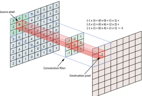
Figure 1.7: The result of a single convolution operation. The process is re-peated by shifting the filter all-over the entire original image.
1.5.1
Building blocks
Convolution
The convolution operation is the core building block of CNNs. A convolution over an image requires a convolution matrix (or filter) which is moved across the image. The result of a single convolution operation is the sum of all products between the filter elements and the corresponding pixels.
Usually, the results are stored in a new image, which represents the response of the original image to the filter used. Changing the filter results in different features being extracted from the initial image. The resulting image’s size depends on the size of the original image and the size of the filter. More formally:
wo =wi−wf + 1 and ho =hi−hf + 1 (1.32)
where:
• wo and ho are the width and height of the image resulting from
convolu-tion.
• wi and hi are the width and height of the input image.
Often CNNs have to deal with 3D input, such as RGB images. In those cases, the filter is also 3D, with a depth equal to the input’s number of input channels. The output of a single convolution operation is still a number. Generally, more than one filter is used in each convolution layer, with the aim of deriving different features from the same input. Thus, each convolution layer can be represented as a bank of filters, and its output is composed ofkdifferent output images (feature maps), with k= number of filters.
In a convolutional neural network the filters are automatically learned during the training phase. This means that the network learns what features are the most crucial, and how to extract them from an image.
The two most important characteristic of convolutional neural networks are the sharing of weights among neurons in the same layer, and the locality of the connection. Every neuron in a convolutional layer is connected with only a small portion of the perceptrons of the previous layers, as defined by the size of the filter. Moreover, the weights are shared among neurons in the same layer, drastically reducing the number of parameters, with respect to an MLP. As an example, in the first convolution layer, assuming 3×3 filters and an RGB input image (C = 3), the filter is characterized only by 3·3·C = 27 weights, so there are only 27 parameter to be learned, regardless the number of neurons in the layer.
Downsampling
The downsampling block is another important module of a CNN. It has the aim of reducing the dimension of the input, in order to lower the number of parameters and give the model more robustness to input changes [10]. The most commonly used downsamplig layer is max pooling. In the max pooling layer, the image is divided into small blocks and every block is condensed to its higher value (see Figure 1.8). Another commonly used downsamplig block isaverage pooling, when the output of a block is the average of all the values within it.
1.5.2
Architecture
Convolutional neural networks are powerful classifiers [27], mainly due to the automatic extraction of relevant feature, which had to be manually extracted before the advent of CNNs. They are extremely suitable when the dimension-ality of the data is particularly high, as in images.
1.5. Convolutional Neural Networks 27
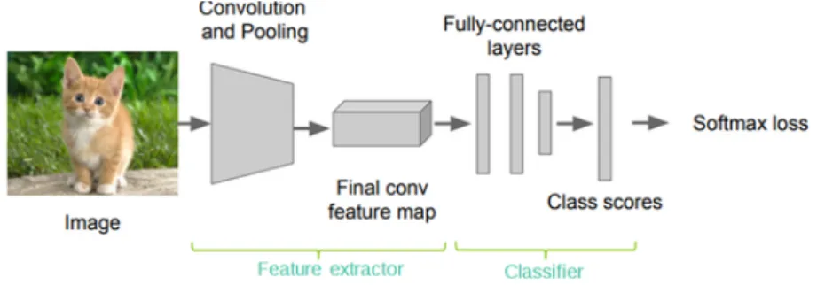
Figure 1.8: The result of a max pool operation using 2x2 blocks. A CNN is typically composed of two modules: the feature extractor and the classifier. The input, which usually consists of RGB images, is given to the former module, which produces a feature vector of k elements. This array is then delivered to a fully connected neural network, which assigns a class to the input, relying on the extracted features.
Figure 1.9: General CNN architecture, composed of a feature extractor and a classifier.
The classifier is usually a fully-connected multilayer perceptron, with as many neurons in the output layer as the number of classes. The feature extractor, by contrast, generally consists of many convolutional layers, each of which are usually followed by an activation layer (ReLU is commonly used as an activation function). Every s block of convolution plus activation, there is a downsampling layer, which reduces the dimensionality of the feature maps. The value of s depends on the network, and can even vary inside the network itself, but usually ranges from one to three. In some cases, only convolution plus activation is used [28]; on uch occasions, the CNN is commonly called a
fully convolutional network (FCN).
The training phase of a convolutional neural network is similar to the one described in subsection 1.3.4. Backpropagation is used as in MLPs and the
weight are updated in a similar manner.
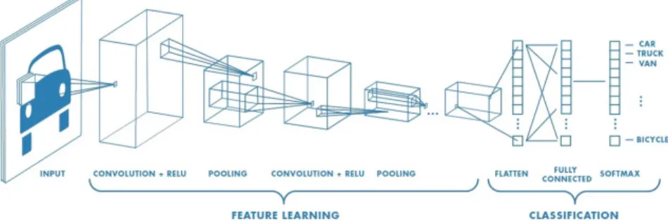
Figure 1.10: A typical CNN architecture, with a pooling layer after every convolution plus ReLU block. The total number of layers in the network is a design choice, and can widely vary from different models.
1.5.3
Applications
As stated at the beginning of this section, CNNs are widely used for image processing. This trend started in 2012, whenAlexNet won theImageNet Large Scale Visual Recognition Challenge [29]. Since then, convolutional neural net-works have become the standard for image-related tasks, such as classification or object detection.
The feature extractor module can be used for transfer learning. A trained CNN is a powerful feature extractor: changing only the classifier and training it, keeping the former module fixed, is often much faster than training a CNN from scratch.
Another application of CNN is within a class of methods named encoders. In general terms, an encoder is a device that converts information from one format to another, and can be mathematically expressed as a function: φ : A → B
whereA and B are two different spaces (e.g. image space and feature space). The inverse operation of encoding is decoding, which can be expressed as:
ψ : B → A. The purpose of encoding is to compress data into a short code in a latent space. If the encoding is carried out properly, the latent code should contain only the most important features of the data, ignoring noise or unimportant aspects. The latent space can also be used for data editing. For instance, if an encoder has learned how to represents concepts like acat and
flying, those codes can be mixed in the feature space in order to generate a
flying cat after decoding, even if neither the encoder nor the decoder has ever seen a flying cat [30]. Often a single CNN acts both as encoder and as decoder. In this case, the model is called an autoencoder. Autoencoders are one of the
1.5. Convolutional Neural Networks 29 most active research topics in deep learning [10], and are predominantly used for representation learning.
2
Generative Adversarial
Networks
The most interesting idea in the last 10 years in machine learning.
– Yann LeCun, Director of AI research at Facebook
In this chapter, a description of Generative adversarial networks (GANs) is provided, starting from the basic concepts that led to the development of the GAN model. Then, the procedure used to train such models is described, focusing on the differences and problems when compared to classical neural networks, and presenting some solutions to them. At the end of the chapter, the problem of evaluation is discussed , which is common to many generative models.
2.1
Generative Models
In statistical classification, as in machine learning, there are two main types of model: discriminative andgenerative models [8]. Given an observable variable
X, and a target variable Y (i.e X represents the actual data, whileY are the labels), a discriminative model is a model of the targetY given an observation
x ∈ X, symbolically P(Y|X = x). A discriminative model, in brief, learns how to classify every pattern x to the correct label y. Methods like support vector machines (SVMs) and neural networks fall into this category.
On the other hand, generative models are statistical models ofjoint probability distribution P(X, Y). A generative model learns the intrinsic distribution of
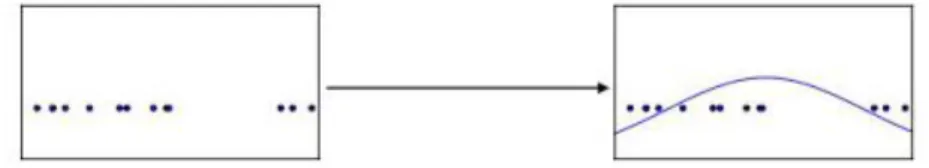
Figure 2.1: The operation of density estimation performed by a generative Gaussian model over mono-dimensional data. [31]
data, allowing it to generate new data according to the real data distribution (this is why these models are called generative). In short, a generative model, given a training set consisting of samples drawn from a distribution pdata,
learns how to represent and estimate such a distribution, and the result is a probability distributionpmodel, which will hopefully be similar to pdata [31].
It is important to report that, given the Bayes theorem:
P(Y|X) = P(X|Y)P(Y)
P(X) and P(X|Y)P(Y) = P(X, Y) (2.1) the result is that:
P(Y|X) = P(X, Y) P(X) . (2.2) Since P(X) = X y P(X, Y =y) (2.3)
the discriminative model can be directly derived from the generative one:
P(Y|X) = P P(X, Y)
yP(X, Y =y)
. (2.4)
Therefore, given a generative model, it is possible to derive a discriminative model. Moreover, the former contains more information than the latter, and it can be used to discover complex relationships between X and Y, such as in the case of multi-modal outputs (given an input x ∈ X, more than one element of Y is correct; i.e. x is a frame in a video and y is the predicted next frame). However, for classification purposes, discriminitavive models are usually preferred, due to their higher accuracy, if they are trained with large datasets [32].
2.1. Generative Models 33
2.1.1
Maximum likelihood estimation
In the previous section, it was stated that generative models produce a prob-ability distribution pmodel which should resemble the real distribution of data
pdata. Likelihood provides a metric for comparing two probability
distribu-tions, and the maximum likelihood estimator can be used to find the optimal parameters of the generative model.
The likelihood of a model is given byl =Qn
i=1pmodel(x(i), θ), where x(i) is the
i-th element of the dataset, and θ represents the parameters of the model. To simplify computations, the log likelihood is often taken into consider-ation, and therefore the product is transformed into a sum of logarithms:
l = Pn
i=1logpmodel(x
(i), θ). The best model is the one with the maximum
likelihood, so: θ∗ = arg max θ n X i=1 logpmodel(x(i), θ) = arg max θ E
x∼pˆdatalogpmodel(x, θ) (2.5)
where ˆpdata is the distribution defined by the training data. The maximum
likelihood estimator can be interpreted as a method to minimize the dissim-ilarity between ˆpdata and pmodel, similarly to the KL divergence. Usually, the
optimal parameters are estimated by minimizing the negative of the likelihood; thus:
θ∗ = arg min
θ
−Ex∼pˆdatalogpmodel(x, θ) (2.6)
Note that minimizing the KL divergence between two distributions corresponds precisely to minimizing the cross entropy between them. For this reason, the cross entropy loss defined in subsection 1.3.3 is widely used in many machine learning models.
2.1.2
A taxonomy of generative models
Some generative models do not use maximum likelihood in principle, but they can be examined using a maximum likelihood variant. The main distinction among generative models is between explicit and implicit density models. For a complete review of generative models in relation to GANs see [31].
Explicit density function
Models that are in this category explicitly define the density function pmodel.
For these kind of models, the maximization of the likelihood is straightforward: it is sufficient to use Equation 2.5 and follow the gradient uphill (or downhill if the divergence is used).
The main difficulty with explicit density models is the designing of a model that can capture all the complexity of the data and, at the same time, maintain computational tractability. To confront this challenge, there are two different strategies:
• Tractable explicit models: the density functionpmodelis chosen to be
computationally tractable. Examples of such models are fully-visible be-lief networks, nonlinear independent component analysis and pixelRNN.
• Approximated explicit models: when the distribution of the data cannot be reduced to a tractable pmodel, a intractable one is used, and
approximated with a lower bound L(x, θ) ≤ logpmodel(x, θ).
Maximiz-ing L(x, θ) has almost the same effect as maximizing the likelihood if the two functions are not distant, especially in their optimal point. The most famous example of approximate explicit models is thevariational autoen-coder (VAE). Another kind of models uses theMarkov chain approxima-tion instead of defining a lower-bound function. The most prominent example of these models is the Boltzmann machine [33].
Implicit density function
Some models can be trained without the need to explicitly define a density function. These models interact only indirectly with pmodel, usually sampling
data from it in order to compare the generated data with the training set distribution ˆpdata. In brief, the goal of these types of models is not to learn
how the data is distributed throughout space, but how to generate items that
seem extracted from pdata. Some implicit density models use Markov chains
to draw samples from the implicit pmodel, as generative stochastic networks.
Those models, however, do not scale well to high dimensional space, and they require many steps to generate data. Generative adversarial networks were designed to avoid those problems, so they are able to generate samples in a single step.