Hessian-based model reduction with applications to initial-condition inverse problems

Hessian-Based Model Reduction with Applications

to Initial-Condition Inverse Problems

by

Omar Shahid Bashir

Submitted to the Department of Aeronautics and Astronautics

in partial fulfillment of the requirements for the degree of

Master of Science in Aerospace Engineering

at the

MASSACHUSETTS INSTITUTE OF TECHNOLOGY

September 2007

c

Massachusetts Institute of Technology 2007. All rights reserved.

Author . . . .

Department of Aeronautics and Astronautics

August 23, 2007

Certified by . . . .

Karen E. Willcox

Associate Professor of Aeronautics and Astronautics

Thesis Supervisor

Accepted by . . . .

David L. Darmofal

Associate Professor of Aeronautics and Astronautics

Chair, Committee on Graduate Students

Hessian-Based Model Reduction with Applications to

Initial-Condition Inverse Problems

by

Omar Shahid Bashir

Submitted to the Department of Aeronautics and Astronautics on August 23, 2007, in partial fulfillment of the

requirements for the degree of

Master of Science in Aerospace Engineering

Abstract

Reduced-order models that are able to approximate output quantities of interest of high-fidelity computational models over a wide range of input parameters play an important role in making tractable large-scale optimal design, optimal control, and inverse problem applications. We consider the problem of determining a reduced model of an initial value problem that spans all important initial conditions, and pose the task of determining appropriate training sets for reduced-basis construction as a sequence of optimization problems.

We show that, under certain assumptions, these optimization problems have an explicit solution in the form of an eigenvalue problem, yielding an efficient Hessian-based model reduction algorithm that scales well to systems with states of high di-mension. Furthermore, tight upper bounds are given for the error in the outputs of the reduced models. The reduction methodology is demonstrated for several linear systems, including a large-scale contaminant transport problem.

Models constructed with the Hessian-based approach are used to solve an initial-condition inverse problem, and the resulting initial initial-condition estimates compare fa-vorably to those computed with high-fidelity models and low-rank approximations. Initial condition estimates are then formed with limited observational data to demon-strate that predictions of system state using reduced models are possible given rela-tively short measurement time windows. We show that reduced state can be used to approximate full state given an appropriate reduced basis, meaning that approximate forward simulations of large-scale systems can be computed in reduced space.

Thesis Supervisor: Karen E. Willcox

Acknowledgements

My advisor, Prof. Karen Willcox, has provided so much support with her extensive technical knowledge and her words of encouragement. She has always been completely accessible even when we’re on different continents. I especially want to thank her for helping me to take advantage of every opportunity, and for doing so with my best interests in mind. I am also thankful to Prof. Omar Ghattas for his advice and for allowing me to absorb some of his insight into inverse problems and related topics. I thank Bart van Bloemen Waanders and Judy Hill for answering all my questions and for making my stay at Sandia productive and enjoyable.

My friends in the ACDL were important during the past two years: Tan Bui brought me up to speed in many areas when I was just starting my research, and Garrett Barter was always willing to help as well. JM, Leia, Laslo, David, Josh, Alejandra, Theresa, and Tudor: sorry for bringing Settlers in and damaging your good work habits. It has been fun working with you guys and with all the other students in the lab. I’m also grateful to my roommate Adam Kumpf for asking hard questions about my research when I was stuck. Finally, I thank God for giving me parents who work hard to support me in all my academic pursuits.

This work was made possible by a National Science Foundation Graduate Research Fellowship. It was also supported by the NSF under DDDAS grant CNS-0540186 (program director Dr. Frederica Darema), the Air Force Office of Scientific Research (program manager Dr. Fariba Fahroo), and the Computer Science Research Institute at Sandia National Laboratories.

Contents

2 Model Reduction Framework 19 2.1 Reduction via Projection . . . 19

2.2 Proper Orthogonal Decomposition . . . 23

2.3 Output-Weighted POD for Time-Dependent Problems. . . 24

3 Hessian-Based Construction of Reduced-Order Models 27 3.1 Theoretical Approach . . . 27

3.2 Error Analysis. . . 33

3.3 Large Scale Implementation . . . 34

4 Application: Convection-Diffusion Transport Problem 37 4.1 Two-dimensional model problem. . . 37

4.1.1 Problem description . . . 37

4.1.2 Reduced model performance . . . 40

4.1.3 Ten-sensor case . . . 46

4.1.4 Observations and Recommendations . . . 48

4.2 Contaminant Transport in a 3-D Urban Canyon . . . 51

5 Application: Measurement, Inversion, and Prediction 57 5.1 Estimating the Initial Condition . . . 58

5.1.1 Low-Rank Hessian Approximation. . . 60

5.1.2 Reduced-Order Inverse Problem Solution . . . 61

5.1.3 Inverse Problem Results . . . 62

5.1.4 Implementation Cost Comparison . . . 70

5.2 Using Reduced State to Approximate Full State . . . 72

5.2.1 Comparison of Full State to its Approximation . . . 72

5.2.2 State Approximation in the Inverse Problem Context . . . 74

5.3 State Prediction from Limited Observational Data . . . 76

5.3.1 Time-Limited Estimates of the Initial Condition . . . 78

5.3.2 Time-Limited Inversion Results . . . 79

6 Conclusion 83 6.1 Summary . . . 83

List of Figures

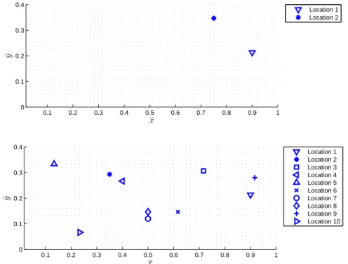
4-1 The computational domain and locations of sensor output nodes. Top: two-sensor case, bottom: ten-sensor case. . . 38

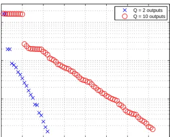
4-2 A comparison of the Hessian eigenvalue spectra of H for the two- and

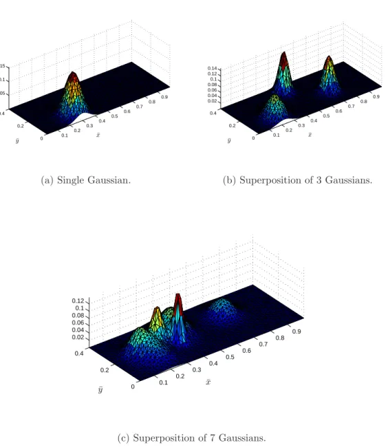
ten-output cases. Pe = 100. . . 40 4-3 Sample test initial conditions used to compare reduced model outputs

to full-scale outputs. . . 42

4-4 Top: Maximum error, εmax, for reduced models computed using

Algo-rithms 1 and 2. Bottom: Error for test initial condition (b), ε. . . 44

4-5 A comparison of full (N = 1860) and reduced (n = 196) outputs for

two-sensor case using test initial condition (b). Pe=1000, ¯λ = 0.01, ¯

µ= 10−4_{, ε= 0.0039. . . . . 44} 4-6 A comparison between full and reduced solutions at sensor location 1

for two different values of ¯µ. Test initial condition (a) was used to generate the data. Pe=10, ¯λ = 0.01, two-sensor case. The output at the first sensor location is plotted here. . . 45

4-7 Lowering ¯λ to increase p, the number of Hessian eigenvector initial

conditions used in basis formation, leads to more accurate reduced-order output. Test initial condition (c) was used with two output

sensors, Pe=100 and ¯µ = 10−4_{. The output at the second sensor}

location is plotted here.. . . 46

4-8 A comparison of the full (N = 1860) and reduced (n = 245) outputs

for all Q= 10 locations of interest. Test initial condition (c) was used to generate these data with Pe = 100, ¯µ= 10−₄

4-9 A measure of the error in six different reduced models of the same system plotted versus their sizes n for the ten-sensor case. The three plots were generated with test initial conditions (a), (b), and (c),

re-spectively. Pe=100,Q= 10 outputs. . . 49

4-10 Building geometry and locations of outputs for the 3-D urban canyon problem. . . 53 4-11 Transport of contaminant concentration through urban canyon at six

different instants in time, beginning with the initial condition shown in upper left. . . 54 4-12 Full (65,600 states) and reduced (137 states) model contaminant

con-centration predictions at each of the six output nodes for the

three-dimensional urban canyon example. . . 55

5-1 The actual initial condition used for the experiments; the goal of solving the inverse problem is to find this distribution from sensor measure-ments. Formed by superposing 10 Gaussian distributions with random centers and standard deviations. . . 63

5-2 The first 150 eigenvalues in the spectra of H+βI and Hr+βI with

β = 0 and β = 0.001. The reduced model used to construct Hr is

the baseline model with ¯λ = 0.1, ¯µ = 10−4_{, and n = 245. P e = 100,} Q= 10 outputs. . . 65 5-3 Error in low-rank and reduced-order initial condition versus actual

ini-tial conditionxa

0 (top) and versus truth initial conditionxt0 (bottom). Data from reduced models formed with baseline values of ¯λ= 0.1 and ¯

µ= 10−4 _{and with strict values of ¯λ= 0.01 and ¯µ= 10}−6 _{are shown.} Unless otherwise stated, the regularization constant for all trials is β = 0.001. P e= 100, Q= 10 outputs. . . 67

5-4 The truth initial condition estimate xt

0 (top) and the reduced-order

estimate xrom

0 . The reduced model used is the baseline model with

¯

λ= 0.1, ¯µ= 10−₄

5-5 The the actual sensor measurements (outputs) compared to y and y_r.

Here, y is generated by solving forward in time with the full-order

equations starting from truth initial condition xt

0; yr is generated by solving forward in time with the reduced-order equations starting from reduced initial condition xrom

0 . Both initial condition estimates are

shown in Figure 5-4. . . 69 5-6 Full-state approximation error with three different reduced-order

mod-els with identical initial conditions. P e= 100, Q= 10 outputs. . . 73

5-7 State at t = 0.4 as calculated by the high-fidelity (top) and by the

reduced-order systems of equations (middle), along with the error

be-tween the two snapshots (bottom). The reduced model (n= 361) with

strict ¯µwas used for this comparison. P e= 100, Q= 10 outputs. . . 75

5-8 At right, full-state approximation error with respect to high-fidelity forward solve starting from the truth initial conditionxt

0. The data are shown for three different reduced-order models with their respective initial conditions xrom

0 . On the left, the same data plotted against

the actual state evolution in the domain, including the truth case for comparison. P e= 100, Q= 10 outputs.. . . 76 5-9 The actual state xa _{in the domain at t = 0.2 (top); the state x}t _as

calculated by the high-fidelity system of equations beginning from the truth initial condition xt

0 (middle); and the state xrom as calculated by the order system of equations beginning from the reduced-order initial condition xrom

0 (bottom). The reduced model (n = 361)

with strict ¯µwas used for this comparison. Note the fine grid associated

with the actual state. P e= 100, Q= 10 outputs. . . 77

5-10 Effect of varying the length of observation time on the error between estimated initial condition and actual initial condition. The baseline and strict reduced-order models are described in Section 5.1.3. P e = 100, Q= 10 outputs. . . 80

5-11 Full-order (truth) and reduced order estimates ˜xt

0 and ˜xrom0 of the

ini-tial condition given a time window of length tf = 0.2. Compare to

Figure 5-4, which shows inversion results using a much longer time

horizon of tf = 1.4. The reduced-order model used is the baseline

List of Tables

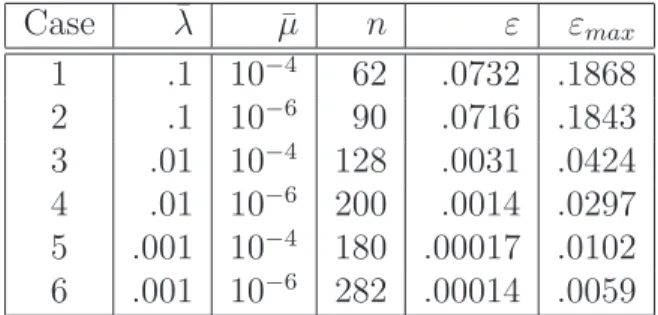
4.1 Properties of various reduced-order models of a full-scale system with

Pe=100 and two output sensors. The errors ε and εmax are defined

in (3.20) and (3.21), respectively; ε is evaluated when each reduced

system (of dimension n) is subjected to test initial condition (c). . . . 41

4.2 Properties of various reduced-order models of a full-scale system with

Pe=1000 and two output sensors. The errors ε and εmax are defined

in (3.20) and (3.21), respectively; ε is evaluated when each reduced

system (of dimension n) is subjected to test initial condition (a). . . . 43

Chapter 1

Introduction

1.1

Motivation

Reduced-order models that are able to approximate outputs of high-fidelity computa-tional models over a wide range of input parameters have an important role to play in making tractable large-scale optimal design, optimal control, and inverse problem ap-plications. For example, consider a time-dependent inverse problem in which the goal is to estimate the initial condition. The constraints are the state equations describing the dynamics of the system, and the objective is the difference between the measured state observations and observations predicted by the state equations starting from the unknown initial condition.

When the physical system being simulated is governed by partial differential equa-tions in three spatial dimensions and time, the forward problem alone (i.e. solution of the PDEs for a given initial condition) may require many hours of supercomputer time. The inverse problem, which requires repeated solution of the forward prob-lem, may then be out of reach in situations where rapid assimilation of the data is required. In particular, when the simulation is used as a basis for forecasting or decision-making, a reduced model that can execute much more rapidly than the high-fidelity PDE simulation is needed. A crucial requirement for the reduced model is that it be able to replicate the output quantities of interest (i.e. the observables) of the PDE simulation over a wide range of initial conditions, so that it may serve as a

surrogate of the high-fidelity PDE simulation during inversion.

One popular method for generating a reduced model is through a projection basis; for example, by proper orthogonal decomposition (POD) in conjunction with the method of snapshots. To build such a reduced order model, one typically constructs a training set by sampling the space of (discretized) initial conditions. When this space is high-dimensional, the problem of adequately sampling it quickly becomes intractable. Fortunately, for many ill-posed inverse problems, many components of the initial condition space have minimal or no effect on the output observables. This is particularly true when the observations are sparse. In this case, it is likely that an effective reduced model can be generated with few sample points. If appropriate sample points can be located, it is possible to form a reduced model which can accept a wide range of initial conditions while providing accurate outputs. The initial-condition sampling issue is therefore the central theme of this thesis.

1.2

Objectives

The primary objectives of this thesis are:

• to present a model reduction approach that is capable of generating reduced

models that provide accurate output replication for a wide range of possible initial conditions;

• to explain the sources of computational cost associated with the new approach;

• to evaluate the approach by forming reduced models of high-fidelity linear

sys-tems and subjecting both full and reduced models to a variety of test initial conditons;

• to demonstrate that the resulting reduced models are well-suited for use in the

efficient solution of initial-condition inverse problems and in the state estimation which often follows in practice.

1.3

Previous Work

Reduction techniques for large-scale systems have generally focused on a projection framework that utilizes a reduced-space basis. Methods to compute the basis in the

large-scale setting include Krylov-subspace methods [18, 19, 24], approximate

bal-anced truncation [25, 32, 33, 36], and proper orthogonal decomposition [16, 29, 35]. Progress has been made in development and application of these methods to opti-mization applications with a small number of input parameters, for example optimal

control [2, 5, 28, 30] and parametrized design of interconnect circuits [15]. In the

case of a high-dimensional input parameter space, the computational cost of deter-mining the reduced basis by these techniques becomes prohibitive unless some sparse sampling strategy is employed.

For initial-condition problems of moderate dimension, a reduction method has been proposed that truncates a balanced representation of the finite-dimensional

Han-kel operator [17]. In [14], POD was used in a large-scale inverse problem setting to

define a reduced space for the initial condition in which to solve the data assimilation problem. In that work, only a single initial condition was used to generate the state solutions necessary to form the reduced basis: either the true initial condition, which does contain the necessary information but would be unavailable in practice, or the background estimate of the initial state, which defines a forecast trajectory that may not be sufficiently rich in terms of state information.

For model reduction of linear time-invariant systems using multipoint rational Krylov approximations, two methods have recently been proposed to choose sample

locations: an iterative method to choose an optimal set of interpolation points [26],

and a heuristic statistically-based resampling scheme to select sample points [34].

To address the more general challenge of sampling a high-dimensional parameter

space to build a reduced basis, the greedy algorithm was introduced in [38]. The

key premise of the greedy algorithm is to adaptively choose samples by finding the location in parameter space where the error in the reduced model is maximal. In

steady incompressible Navier-Stokes equations. In [22, 23], the greedy algorithm

was combined with a posteriori error estimators for parametrized parabolic partial

differential equations, and applied to several optimal control and inverse problems.

1.4

Overview

In this thesis, we present a new methodology that employs an efficient sampling strategy to make tractable the task of determining reduced-order models for large-scale linear initial value problems. Reduced models formed using the Hessian-based methodology provide outputs which are similar to those computed with high-fidelity models. This accurate output replication over a wide range of initial conditions allows the reduced models to be used as surrogates for full-order models in initial-condition inverse problems.

Chapter 2 describes the projection framework used to derive the reduced-order dynamical system. It also provides details of the POD and proposes a new POD variant. We present in Chapter 3 the theoretical approach, leading to the Hessian-based reduction methodology. In Chapter 4, we first demonstrate the efficacy of the approach via numerical experiments on a problem of 2-D convective-diffusive transport. We also present an application to model reduction for 3-D contaminant transport in an urban canyon. Chapter 5 contains a demonstration of reduced-order inverse problem solution. It then illustrates the utility of reduced models for state estimation and prediction. We conclude the thesis with Chapter 6.

Chapter 2

Model Reduction Framework

This chapter first describes the reduced-order models intended for use in place of

high-fidelity or full-order systems. It then summarizes in Section 2.2 the details of

the proper orthogonal decomposition (POD) used throughout this work to generate reduced basis vectors. Finally, a new, output-dependent variant of POD is presented in Section 2.3.

2.1

Reduction via Projection

Consider the general linear discrete-time system

Ex(k+ 1) = Ax(k) +Bu(k), k = 0,1, . . . , T ₋1, (2.1)

y(k) = Cx(k), k = 0,1, . . . , T, (2.2)

with initial condition

x(0) = x0, (2.3)

where x(k)_∈ IRN is the system state at time tk, the vector x0 contains the specified

initial state, and we consider a time horizon from t = 0 to t = tf. The vectors

outputs at timetk. In general, we are interested in systems of the form (2.1)–(2.3) that

result from spatial and temporal discretization of PDEs. In this case, the dimension

of the system, N, is very large and the matricesE _∈IRN×N_,A

∈IRN×N,B

∈IRN×P_,

and C _∈IRQ×N _{result from the chosen spatial and temporal discretization methods.}

A reduced-order model of (2.1)–(2.3) can be derived by assuming that the state

x(k) is represented as a linear combination ofn basis vectors,

ˆ

x(k) = V xr(k), (2.4)

where ˆx(k)_∈IRN is the reduced model approximation of the state x(k) and n_≪N.

The projection matrix V _∈IRN×n contains as columns the orthonormal basis vectors

vi, i.e., V = [v1 v2 · · · vn], and the reduced-order state xr(k) ∈ IRn contains the

corresponding modal amplitudes for time tk. Using the representation (2.4) together

with a Galerkin projection of the discrete-time system (2.1)–(2.3) onto the space

spanned by the basis V yields the reduced-order model with state xr and outputyr,

Erxr(k+ 1) = Arxr(k) +Bru(k), k = 0,1, . . . , T −1, (2.5)

yr(k) = Crxr(k), k= 0,1, . . . , T, (2.6)

xr(0) = VTx0, (2.7)

where Er =VTEV, Ar =VTAV, Br =VTB, and Cr =CV.

Since the system (2.1)–(2.3) is linear, the effects of inputs uand initial conditions

x0 can be considered separately. In this thesis, we focus on the initial-condition

problem and, without loss of generality, assume that u(k) = 0, k = 0,1, . . . , T ₋1.

For convenience of notation, we write the discrete-time system (2.1)–(2.3) in matrix

form as

Ax = Fx0, (2.8)

where x=         x(0) x(1) ... x(T)         , y=         y(0) y(1) ... y(T)         . (2.10)

The matricesA_∈IRN(T+1)×N(T+1),F_∈IRN(T+1)×N, andC_∈IRQ(T+1)×N(T+1) in (2.8) and (2.9) are given by

A=            E 0 _{· · · ·} 0 −A E 0 0 ₋A E . .. ... . .. ... ... 0 0 0 ₋A E            ,F=            E 0 0 ... 0            ,C=            C 0 _{· · · ·} 0 0 C 0 ... 0 C . .. ... . .. ... 0 0 0 C            . (2.11)

Similarly, the reduced-order model (2.5)–(2.7) can be written in matrix form as

A_rx_r = F_rx0, (2.12)

y_r = C_rx_r, (2.13)

where xr and yr are defined analogously toxand yas

xr =         xr(0) xr(1) ... xr(T)         , yr =         yr(0) yr(1) ... yr(T)         . (2.14)

given by Ar =            Er 0 · · · 0 −Ar Er 0 0 ₋Ar Er . .. ... . .. ... ... 0 0 0 ₋Ar Er            ,Fr =            ErVT 0 0 ... 0            , (2.15) Cr=            Cr 0 · · · 0 0 Cr 0 ... 0 Cr . .. ... . .. ... 0 0 0 Cr            .

As an alternative to the discrete-time representation of a system (2.1)–(2.2), a

continuous representation of the form

Mx˙(k) = _Ax(k) +_Bu(k), (2.16)

y(k) = Cx(k), (2.17)

where ˙x is the vector of state derivatives with respect to time, may be available.

Here, _{M ∈} IRN×N_,

A ∈ IRN×N_{, and}

B ∈ IRN×P _{might come from a finite-element}

discretization with mass matrix _M and stiffness matrix _A. We can arrive at the

matrix representation (2.8)–(2.9) in this case by choosing a temporal discretization

method and timestep ∆t, again assuming that u(k) = 0, k = 0,1, . . . , T ₋1 without loss of generality. For example, if the Crank-Nicolson method is chosen, the matrices in (2.11) with

E = _{M −} 1

2∆tA, (2.18)

A = _M+1

can be used in conjunction with (2.8)–(2.9) to solve for system state over time. Note

that Cremains as given in (2.11) since the input-to-output mapping is unchanged.

To form the reduced-order system of equations in this continuous case, the Galerkin

projection is applied to _Mand _A or, equivalently, toE and A:

Er = VTEV, (2.20)

Ar = VTAV. (2.21)

These matrices form the block entries in (2.15); the reduced state can be obtained by

solving (2.12).

In many cases, we are interested in rapid identification of initial conditions from sparse measurements of the states over a time horizon; we thus require a reduced-order model that will provide accurate outputs for any initial condition contained

in some set _X0. Using the projection framework described above, the task therefore

becomes one of choosing an appropriate basis V so that the error between full-order

outputyand the reduced-order outputyr is small for all initial conditions of interest.

2.2

Proper Orthogonal Decomposition

To compute the basis V via POD, a sample set of initial conditions must first be

cho-sen. At each selected initial condition, a forward simulation is performed to generate a set of states, commonly referred to as snapshots. The POD is then applied to the snapshot set in order to form reduced basis vectors. Although the choice of sample

initial conditions is the focus of Chapter 3, we describe the process of forming basis

vectors using the method of snapshots [35] in this section.

Assume that we wish to construct a reduced basis with data frompforward solves

of the high-fidelity system with different initial conditions. The instantaneous state solutions xj_{i ∈} IRN×1, i = 0,1, . . . , T, j = 1,2, . . . , p are collected in the snapshot matrix X _∈IRN×p(T+1)_.

best represent the given snapshots inX [9]. This occurs when then basis vectors are

taken to be the n most dominant eigenvectors of XXT _{or, equivalently, the first n}

left singular vectors of X.

The POD minimizes the quantity

ˆ E = T+1 X i=0 p X j=1 xj_{i −}V VTxj_iT xj_{i −}V VTxj_i, (2.22)

for a fixed number of basis vectors. Eˆ represents the error between the original

snapshots and their representations in the reduced space. This error is also equal to the sum of the squares of the singular values corresponding to the singular vectors not included in the basis,

ˆ E = p(T+1) X k=n+1 σ2_k, (2.23)

where σk is the kth singular value of X.

2.3

Output-Weighted POD for Time-Dependent

Problems

In the classical POD described in Section 2.2, the basis vectors are chosen such that

they minimize the state error in a least-squares sense. However, the outputs do not

influence the basis construction as they do in the weighted POD method we describe in this section.

The idea of weighting snapshots to improve basis quality has been explored before

[13]. It has been emphasized that weighting the snapshots can have a significant

impact on the selection of dominant modes [21]. One such implementation involves

an integer weighting scale such that multiple copies of strongly-weighted snapshots

are included in the data set before POD is applied [11].

Regardless of how the weights are calculated, we first summarize the approach

of the data ¯x _∈ IRN is computed using a linear combination of the snapshots x(i).

If, for simplicity, we are only interested in the T + 1 snapshots from a single forward

solve, then ¯ x= T X i=0 ωix(i), (2.24)

where the snapshot weights ωi are chosen such that 0 < ωi < 1,

PT

i=0ωi = 1. A

modified snapshot matrix ˇX can then be computed using the ensemble average:

ˇ

X = [x(0)₋x, x¯ (1)₋x, . . . , x¯ (T)₋x¯]. (2.25)

If W is a defined as a diagonal matrix of weights ω0 to ωT, then the weighted POD

basis vectors are the eigenvectors ˇvi in the eigenvalue problem

ˇ

XWXˇTvˇi = ˇσivˇi, i= 1,2, . . . , N, (2.26)

where ˇσi are the eigenvalues of ˇXWXˇT.

We propose a new choice of weights which takes into account the current and future

output response associated with each snapshot. The motivation behind this choice is the assumption that the least valuable snapshots for reduced basis formation are those which, when used as initial conditions, cause little or no output response. Those which cause a relatively large output over time are considered the most important snapshots. This distinction allows us to form a quantitative weighting method. Specifically, the

non-normalized weights ˆωi are given by

ˆ

ωi =

Z tf

ti

||y(t)_||2₂dt, i= 0,1, . . . , T, (2.27)

where ti is the time corresponding to snapshot i, and tf is the final time at which

snapshots are collected. The output vector y(t) _∈ IRQ can be calculated via the

state-to-output mapping matrix C. To normalize the weights,

ωi = ˆ ωi ˆ ωmax , (2.28)

where ˆωmax is the maximum non-normalized weight in the snapshot set. Since the

algorithms presented in Chapter 3 require forward solves for many different initial

conditions, the snapshot sets for each of these initial conditions are kept separate so that weights are calculated independently within each set; however, normalizing every

snapshot by the largest ˆωmax across all snapshot sets may also be a valid approach.

The former method is used in this work.

Since all snapshots x are already collected before the calculation of weights, the

only additional costs involved in finding each weight are the single matrix-vector

multiplication y = Cx and a numerical integration to approximate the

continuous-time integral in (2.27). The intended benefit of the output-weighted POD is the

construction of bases which are similar in size to those created with classical POD but which provide a higher degree of output accuracy when both are subjected to test initial conditions. Alternatively, the method can be viewed as an attempt to reduce the number of basis vectors needed to achieve a certain level of accuracy. The

Chapter 3

Hessian-Based Construction of

Reduced-Order Models

In this chapter, a methodology to determine a basis that spans the space of important initial conditions is presented. It has been shown that in the case of systems that are linear in the state, POD is equivalent to balanced truncation if the snapshots are

computed for all possible initial conditions [31]. Since sampling all possible initial

conditions is not feasible for large-scale problems, we propose an adaptive approach to identify important initial conditions that should be sampled. The approach is

motivated by the greedy algorithm of [38], which proposed an adaptive approach to

determine the parameter locations at which samples are drawn to form a reduced basis. For the linear finite-time-horizon problem considered here, we show that the greedy algorithm can be formulated as an optimization problem that has an explicit solution in the form of an eigenvalue problem.

3.1

Theoretical Approach

Our task is to find an appropriate reduced basis and associated reduced model: one that provides accurate outputs for all initial conditions of interest. We define an

optimal basis, V∗

, to be one that minimizes the maximal L2 error between the

conditions, V∗ = arg min V xmax0∈X0 (y−yr) T (y₋yr) (3.1) where Ax = Fx0, (3.2) y = Cx, (3.3) Arxr = Frx0, (3.4) yr = Crxr. (3.5)

For this formulation, the only restriction that we place on the set _X0 is that it

con-tain vectors of unit length. This prevents unboundedness in the optimization problem, since otherwise the error in the reduced system could be made arbitrarily large.

Natu-rally, because the system is linear, the basis V∗

will still be valid for initial conditions of any finite norm.

A suboptimal but computationally efficient approach to solving the

optimiza-tion problem (3.1)–(3.5) is inspired by the greedy algorithm of [38]. Construction

of a reduced basis for a steady or unsteady problem with parameter dependence,

as considered in [37, 22], requires a set of snapshots, or state solutions, over the

parameter–time space. The greedy algorithm adaptively selects these snapshots by finding the location in parameter–time space where the error between the full-order and reduced-order models is maximal, updating the basis with information gathered from this sample location, forming a new reduced model, and repeating the process.

In the case of the initial-condition problem (3.1)–(3.5), the greedy approach amounts

to sampling at the initial condition x∗

0 ∈ X0 that maximizes the error in (3.1).

The key step in the greedy algorithm is finding the worst-case initial conditionx∗

0,

which we achieve by solving the modified optimization problem,

x∗

0 = arg max

x0∈X0

where Ax = Fx0, (3.7)

y = Cx, (3.8)

A_rx_r = F_rx0, (3.9)

y_r = C_rx_r. (3.10)

Equations (3.6)–(3.10) define a large-scale optimization problem, which includes the

full-scale dynamics (3.7), (3.8) as constraints. The approach taken in [37, 22] is to replace these constraints with error estimators, so that the full-scale model does not

need to be invoked during solution of the optimization problem. Further, in [37, 22],

the optimization problem (20)-(24) is solved by a grid-search technique that addresses problems associated with non-convexity and non-availability of derivatives.

In this chapter, we exploit the linearity of the state equations to eliminate the full-order and reduced-full-order states and yield an equivalent unconstrained optimization

problem. Eliminating the constraints (3.7)–(3.10) by solving for the full and reduced

states yields

x∗

0 = arg max_x0∈X0 xT0Hex0, (3.11)

where

He= CA−1F₋C_rA−_r1F_rT CA−1F₋C_rA−_r1F_r. (3.12)

It can be seen that (3.11) is a quadratic unconstrained optimization problem with

Hessian matrix He _{∈ IR}N×N_{. From (3.12), it can be seen that H}e _{is a symmetric}

positive semi-definite matrix that does not depend upon the state or initial condition.

The eigenvalues of He _{are therefore non-negative. Since we are considering initial}

conditions of unit norm, the solution x∗

0 maximizes the Rayleigh quotient; therefore,

the solution of (3.11) is given by the eigenvector ze

1 corresponding to the largest

eigenvalue λe

1 of He:

Hez₁e=λe₁z₁e. (3.13)

The eigenvectorze

1 is the initial condition for which the error in reduced model output

These ideas motivate the following basis-construction algorithm for the initial condition problem.

Algorithm 1 Greedy Reduced Basis Construction

Initialize with V = 0, so that the initial reduced-order model is zero.

1. For the error Hessian matrix, He _{as defined in (3.12), find the eigenvector z}e 1

with largest eigenvalue λe 1.

2. Set x0 =z1e and compute the corresponding solution x using (2.8).

3. Update the basis V by adding the new information from the snapshots x(k),

k = 0,1, . . . , T.

4. Update the reduced model using the new basis and return to Step 1.

In Step 3 of Algorithm 1, the basis could be computed from the snapshots, using,

for example, the POD. A rigorous termination criterion for the algorithm is available in the form of an error bound, which will be discussed below. It should be noted

that, while the specific form of Algorithm1applies only in the linear case, the greedy

sampling concept is applicable to nonlinear problems. In the general nonlinear case,

one would solve an optimization problem similar in form to (3.6)–(3.10), but with

the appropriate nonlinear governing equations appearing as constraints. In this case, the explicit eigenvalue solution to the optimization problem would not hold; instead, one would use a method that is appropriate for large-scale simulation-constrained

optimization (see [3]) to solve the resulting optimization problem.

Under certain assumptions, the form of He _{in (3.11) can be simplified, leading to}

an algorithm that avoids construction of the reduced model at every greedy iteration. We proceed by decomposing a general initial condition vector as

x0 =xV0 +x ⊥

where xV

0 is the component of x0 in the subspace spanned by the current basis V,

and x⊥

0 is the component of x0 in the orthogonal complement of that subspace.

Sub-stituting (3.14) into the objective function (3.11), we recognize that F_rx⊥

0 = 0, using

the form ofFr given by (2.15) and that, by definition,VTx⊥0 = 0. The unconstrained

optimization problem (3.11) can therefore be written as

x∗ 0 = arg max x0∈X0 CA −1_FxV 0 +CA −1_Fx⊥ 0 −CrA−r1FrxV0 T CA−1FxV₀ +CA−1Fx⊥ 0 −CrA−r1FrxV0 . (3.15)

The expression (3.15) can be approximated by assuming that

CA−1FxV₀ =CrA −₁

r FrxV0, (3.16)

which means that for initial conditions xV

0 in the space spanned by the basis, we

assume that the reduced output exactly matches the full output, i.e. y=y_r. An

ap-proach to satisfying this condition will be described shortly. Using the approximation (3.16), we can rewrite (3.11) as x∗ 0 = arg max x⊥ 0∈X0 x⊥ 0 T Hx⊥ 0, (3.17) where H = CA−1FT CA−1F. (3.18)

H _∈IRN×N _{is now the Hessian matrix of the full-scale system, and does not depend on}

the reduced-order model. As before,H is a symmetric, positive semi-definite matrix

that does not depend upon the state or initial condition.

If we choose to initialize the greedy algorithm with an empty basis, V = 0, then

the maximizer of (3.17) on the first greedy iteration is given by the eigenvector of H

corresponding to the largest eigenvalue. We denote this initial condition by z1 and

note that z1 satisfies

where λ1 is the largest eigenvalue of H. We then set V =z1. Under the assumption

that (3.16) holds, on the second greedy iteration we would therefore seek the initial

condition that maximizes (3.17). Clearly, this initial condition, which should be

orthogonal to z1, is given by z2, the eigenvector of H corresponding to the second

largest eigenvalue.

Returning to assumption (3.16), this condition can be satisfied if we include in the

basis not just the sequence of optimal initial conditions x∗

0 ={z1, z2, . . .}, but rather

the span of allsnapshots (i.e. instantaneous state solutions contained in x) obtained

by solving (2.8) for each of the seed initial conditions z1, z2, . . .. The approximation

(3.16) will then be accurate, provided the final time tf is chosen so that the output

y(k) is small fork > T. If the output is not small fork > T, then a snapshot collected at some time t_k¯, where ¯k < T but ¯k is large, will be added to the basis; however, if

that state were then used as an initial condition in the resulting reduced-order model,

the resulting solution yr would not necessarily be an accurate representation of y.

This is because the basis would not contain information about system state evolution

after time tT−¯k. In that case, (3.16) would not hold. Further, by including both the

initial conditions, zi, and the corresponding snapshots, x, in the basis, the sequence

of eigenvectors zi will no longer satisfy the necessary orthogonality conditions; that

is, the second eigenvector z2 may no longer be orthogonal to the space spanned by

the basis comprisingz1 and its corresponding state solutions. This is because setting

x0 =z1 and computingxwill likely lead to some states that have components in the

direction of z2. We would therefore expect this simplification to be more accurate

for the first few eigenvectors, and become less accurate as the number of seed initial conditions is increased.

These simplifications lead us to an alternate “one-shot” basis-construction algo-rithm for the initial condition problem. This algoalgo-rithm does not solve the

optimiza-tion problems (3.1)–(3.5) or (3.6)–(3.10) exactly, but provides a good approximate

solution to the problem (3.6)–(3.10) under the conditions discussed above. We use

the dominant eigenvectors of the Hessian matrix H to identify the initial-condition

vectors are in turn used to initialize the full-scale discrete-time system to generate a set of state snapshots that are used to form the reduced basis.

Algorithm 2 One-Shot Hessian-Based Reduced Basis Construction

1. For the full-order Hessian matrix,H as defined in (3.18), find thepeigenvectors

z1, z2, . . . , zp with largest eigenvalues λ1 ≥λ2 ≥. . .≥ λp ≥λp+1 ≥ . . .≥λN ≥

0.

2. For i = 1, . . . , p, set x0 = zi and compute the corresponding solution xi using

(2.8).

3. Form the reduced basis as the span of the snapshots xi_{(k), i = 1,2, . . . , p, k =}

0,1, . . . , T.

Steps 2 and 3 in Algorithm 2 allow us to (approximately) satisfy the assumption

(3.16) by including not just the initial conditions z1, z2, . . . , zp in the basis but also

the span of all snapshots generated from those initial conditions. The basis could be computed from the snapshots, using, for example, the POD.

3.2

Error Analysis

A direct measure of the quality of the reduced-order model is available using the

analysis framework described above. We define the error,ε, due to a particular initial

condition x0 as ε=_||y₋yr||2 = CA−1F₋CrA −₁ r Fr x0 2. (3.20)

For a given reduced model, the dominant eigenvector of He _{provides the worst-case}

initial condition. Therefore, the value of the maximal error εmax (for an initial

con-dition of unit norm) is given by

εmax =

p

λe

whereλe

1 is the largest eigenvalue of the error HessianHe, defined by (3.12). The value

εmax provides both a measure on the quality of the reduced model and a quantitative

termination criterion for the basis-construction algorithm.

In Algorithm 1, εmax is readily available, and thus can be used to determine how

many cycles of the algorithm to perform, i.e. the algorithm would be terminated when

the worst-case error is sufficiently small. In Algorithm 2, it is computationally more

efficient to select p, the number of seed initial conditions, based on the decay rate of

the full Hessian eigenvalues λ1, λ2, . . . and to compute all the necessary eigenvectors

z1, z2, . . . , zpat once. Once the reduced model has been created using Algorithm2, the

error HessianHe _{can be formed and the error criterion (3.21) checked to determine if}

further sampling is required. While Algorithm1 is expected to reduce the worst-case

error more quickly, the one-shot Algorithm 2 is attractive since it depends only on

the large-scale system properties and thus does not require us to build the reduced model on each cycle.

We also note that the eigenvectors of H = (CA−1_F)T _(CA−1_{F) are equivalent}

to the (right) singular vectors of CA−1F. Since the latter quantity serves as an

input-output mapping, use of its singular vectors for basis formation is intuitively

attractive. It is also interesting to note that the Hessian H may be thought of as a

finite-time observability Gramian [4].

3.3

Large Scale Implementation

We first discuss the implementation of Algorithm 2 in the large-scale setting, and

then remark on the differences for Algorithm 1.

Algorithm2is a one-shot approach in which all of the eigenpairs can be computed

from the single Hessian matrix H in (3.18). This matrix can be formed explicitly by

first forming A−1_{F, which requires N “forward solves” (i.e. solutions of}

forward-in-time dynamical systems with A as coefficient matrix), where N is the number

of initial condition parameters; or else by first forming A−T_CT_{, which requires Q}

coefficient matrix), where Qis the number of outputs. For large-scale problems with high-dimensional initial condition and output vectors, explicit formation and storage

of H is thus intractable. (A similar argument can be made for the intractability of

computing the singular value decomposition of CA−1_{F.) Even if H could be formed}

and stored, computing its dominant spectrum would be prohibitive, since it is a dense

matrix of order N _×N.

Instead, we use a matrix-free iterative method such as Lanczos to solve for the

dominant eigenpairs of H. Such methods require at each iteration a matrix–vector

product of the form Hwk for some wk, which is formed by successive multiplication

of vectors with the component matrices that make up the Hessian in (3.18). At each

iteration, this amounts to one forward and one adjoint solve involving the system A.

When the eigenvalues are well-separated, convergence to the largest eigenvalues ofH

is rapid. Moreover, when the spectrum decays rapidly, only a handful of eigenvectors

are required by Algorithm 2. Many problems have Hessian matrices that are of low

rank and spectra that decay rapidly, stemming from the limited number of initial conditions that have a significant effect on outputs of interest. For such problems the number of Lanczos iterations required to extract the dominant part of the spectrum

is often independent of the problem size N.

Under this assumption, we can estimate the cost of Step 1 of Algorithm 2 (which

dominates the cost) in the case when the dynamical system (2.8)–(2.9) stems from

a discretized parabolic PDE. The cost of each implicit time step of a forward or adjoint solve is usually linear or weakly superlinear in problem size, using modern

multilevel preconditioned linear solvers. Therefore for T time steps, overall work for

a forward or adjoint solve scales as T N1+α_{, with α usually very small. For a 3-D}

spatial problem, a number of time steps on the order of the diameter of the grid,

and an optimal preconditioner, this gives_O(N4/3_{) complexity per forward solve, and}

hence per Lanczos iteration. Assuming the number of Lanczos iterations necessary to extract the dominant part of the spectrum is independent of the grid size, the overall

complexity remains _O(N4/3_{). (Compare this with straightforward formation of the}

O(N3_{) work.)}

Algorithm 1 is implemented in much the same way. The main difference is that

the error Hessian He _{replaces the Hessian H, and we find the dominant eigenpair}

of each of a sequence of eigenvalue problems, rather than finding p eigenpairs of the

single Hessian H. Each iteration of a Lanczos-type solver for the eigenvalue problem

in Algorithm 1 resembles that of Algorithm 2, and therefore the costs per iteration

are asymptotically the same. It is more difficult to characterize the number of greedy iterations, and hence the number of eigenvector problems, that will be required using

Algorithm1. However, to the extent that the assumptions outlined in Section3.1hold,

the number of greedy iterations will correspond roughly to the number of dominant

eigenvalues of the full Hessian matrix H. As reasoned above, the spectrum of H is

expected to decay rapidly for the problems of interest here; thus, convergence of the greedy reduced basis construction algorithm is expected to be rapid.

Chapter 4

Application: Convection-Diffusion

Transport Problem

In this chapter, the model reduction methodology described in Chapter 3 is assessed

for a contaminant transport problem. We first consider in Section 4.1 the case of a

simple two-dimensional domain, which leads to a system of the form (2.8) of moderate

dimension; in Section 4.2 a large-scale three-dimensional example will be presented.

4.1

Two-dimensional model problem

4.1.1

Problem description

The physical process is modeled by the convection-diffusion equation,

∂w ∂t +~v· ∇w−κ∇ 2_{w = 0 in Ω} ×(0, tf), (4.1) w = 0 on ΓD ×(0, tf), (4.2) ∂w ∂n = 0 on ΓN ×(0, tf), (4.3) w = w0 in Ω for t= 0, (4.4)

wherew is the contaminant concentration (which varies in time and over the domain

0.1 0.2 0.3 0.4 0.5 0.6 0.7 0.8 0.9 1 0 0.1 0.2 0.3 0.4 ¯ x ¯ y Location 1 Location 2 0.1 0.2 0.3 0.4 0.5 0.6 0.7 0.8 0.9 1 0 0.1 0.2 0.3 0.4 ¯ x ¯ y Location 1 Location 2 Location 3 Location 4 Location 5 Location 6 Location 7 Location 8 Location 9 Location 10

Figure 4-1: The computational domain and locations of sensor output nodes. Top: two-sensor case, bottom: ten-sensor case.

and w0 is the given initial condition. Homogeneous Dirichlet boundary conditions

are applied on the inflow boundary ΓD, while homogeneous Neumann conditions are

applied on the other boundaries ΓN.

Figure4-1 shows the computational domain for the two-dimensional contaminant

transport example. The velocity field is taken to be uniform, constant in time, and

directed in the positive ¯x-direction as defined by Figure 4-1. The inflow boundary,

ΓD, is defined by ¯x= 0, 0≤y¯≤0.4; the remaining boundaries comprise ΓN.

A Streamline Upwind Petrov-Galerkin (SUPG) [10] finite-element method is

em-ployed to discretize (4.1) in space using triangular elements. For the cases considered

here, the spatial mesh has N = 1860 nodes. The Crank-Nicolson method is used to

discretize the equations in time. This leads to a linear discrete-time system of the

form (2.8), where the state vector x(k) _∈ IR1860 contains the values of contaminant

concentration at spatial grid points at time tk. For all experiments, the timestep

convection across the length of the domain, wastf = 1.4.

The matrix A in (2.8) depends on the velocity field and the Peclet number, Pe,

which is defined as

Pe = vcℓc

κ , (4.5)

where the characteristic velocity vc is taken to be the maximum velocity magnitude

in the domain, while the domain length is used as the characteristic length ℓc. The

uniform velocity field described above was used in all experiments, but Pe was varied. Increasingly convective transport scenarios corresponding to Peclet numbers of 10, 100, and 1000 were used to generate different full-scale systems.

The outputs of interest are defined to be the values of concentration at selected

sensor locations in the computational domain. Figure 4-1 shows two different sensor

configurations that were employed in the results presented here.

The first step in creating a reduced model with Algorithm2is to computep

domi-nant eigenvectors of the full-scale Hessian matrix H. Figure4-2shows the eigenvalue

spectra ofH for the two-sensor case and the ten-sensor case. The relative decay rates

of these eigenvalues are used to determinep, the number of eigenvectors used as seed

initial conditions. We specify the parameter ¯λ, and apply the criterion that the jth

eigenvector of H is included if λj/λ1 >¯λ.

Figure4-2demonstrates that the decay rate of the dominant eigenvalues is related

to the number and positioning of output sensors. For the two-output case, the two

dominant eigenvalues λ1 and λ2 are of almost equal magnitude; analogous behavior

can be seen for the first ten eigenvalues in the ten-output case. This is consistent with the physical intuition that similarly important modes exist for each of the out-put sensors. For instance, a mode with initial concentration localized around one particular sensor is of similar importance as another mode with high concentration near a different sensor.

0 10 20 30 40 50 60 70 80 10−3 10−2 10−1 100 Eigenvalue index Eigenvalue magnitude Q = 2 outputs Q = 10 outputs

Figure 4-2: A comparison of the Hessian eigenvalue spectra of H for the two- and

ten-output cases. Pe = 100.

4.1.2

Reduced model performance

Once thep seed eigenvectors have been computed, the corresponding state solutions,

x1,x2, . . . ,xp, are computed from (2.8) using each eigenvector in turn as the initial

condition x0. The final step in Algorithm 2 requires the formation of the reduced

basis from the span ofx1,x2, . . . ,xp. We achieve this by aggregating all state solutions

xi_{(k), i = 1,2. . . , p, k= 0,1, . . . , T into a snapshot matrixX ∈IR}N×(T+1)p _{and using}

the classical (non-weighted) POD to select the n basis vectors that most efficiently

span the column space of X. The number of POD basis vectors is chosen based on

the decay of the POD eigenvalues µ1 ≥µ2 ≥ · · · ≥µ(T+1)p ≥0. As above, we define

a parameter ¯µ, and apply the criterion that the kth POD basis vector is retained if

µk/µ1 >µ¯.

The resulting reduced models given by (2.12), (2.13) can be used for any initial

condition x0; to demonstrate the methodology we choose to show results for initial

conditions comprising a superposition of Gaussian functions. Each Gaussian is defined by

x0(¯x,y¯) =

1

σ√2πe

Case ¯λ µ¯ n ε εmax 1 .1 10−₄ 62 .0732 .1868 2 .1 10−6 _{90 .0716 .1843} 3 .01 10−4 _{128 .0031 .0424} 4 .01 10−₆ 200 .0014 .0297 5 .001 10−4 _{180 .00017 .0102} 6 .001 10−6 _{282 .00014 .0059}

Table 4.1: Properties of various reduced-order models of a full-scale system with

Pe=100 and two output sensors. The errors ε and εmax are defined in (3.20) and

(3.21), respectively; ε is evaluated when each reduced system (of dimension n) is

subjected to test initial condition (c).

where (¯xc,y¯c) defines the center of the Gaussian and σ is the standard deviation.

All test initial conditions are normalized such that _||x0||2 = 1. Three sample initial

condition functions that are used in the following analyses are shown in Figure 4-3

and are referred to by their provided labels (a), (b), and (c) throughout.

Tables 4.1 and 4.2 show sample reduced model results for various cases using

the two-sensor configuration shown in Figure 4-1. The error ε is defined in (3.20)

and computed for one of the sample initial conditions shown in Figure 4-3. It can

be seen from the tables that a substantial reduction in the number of states from

N = 1860 can be achieved with low levels of error in the concentration prediction at

the sensor locations. The tables also show that including more modes in the reduced

model, either by decreasing the Hessian eigenvalue decay tolerance ¯λor by decreasing

the POD eigenvalue decay tolerance ¯µ, leads to a reduction in the output error.

Furthermore, the worst case error in each case, εmax, is computed from (3.21) using

the maximal eigenvalue of the error Hessian, He_{. It can also be seen that inclusion}

of more modes in the reduced model leads to a reduction in the worst-case error.

Figure 4-4 shows a comparison between reduced models computed using

Algo-rithm 1 and Algorithm 2. The model sizes n increase with the number p of

eigen-vectors of either H or He _{used as seed initial conditions. For both algorithms, the}

maximum error εmax and the error resulting from a forward solve with initial

0.1 0.2 0.3 0.4 0.5 0.6 0.7 0.8 0.9 0 0.2 0.4 0.05 0.1 0.15 ¯ x ¯ y

(a) Single Gaussian.

0.1 0.2 0.3 0.4 0.5 0.6 0.7 0.8 0.9 0 0.2 0.4 0.02 0.04 0.06 0.08 0.1 0.12 0.14 ¯ x ¯ y (b) Superposition of 3 Gaussians. 0.1 0.2 0.3 0.4 0.5 0.6 0.7 0.8 0.9 0 0.2 0.4 0.02 0.04 0.06 0.08 0.1 0.12 ¯ x ¯ y (c) Superposition of 7 Gaussians.

Figure 4-3: Sample test initial conditions used to compare reduced model outputs to full-scale outputs.

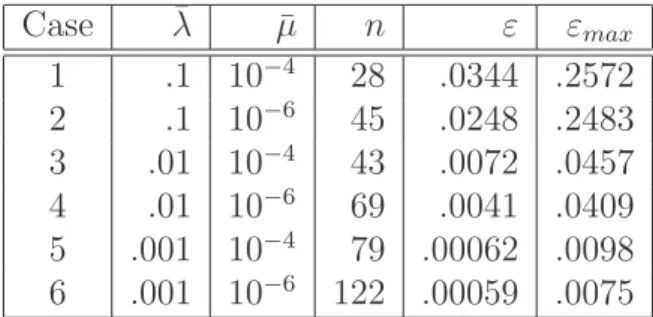
Case ¯λ µ¯ n ε εmax 1 .1 10−₄ 28 .0344 .2572 2 .1 10−6 _{45 .0248 .2483} 3 .01 10−4 _{43 .0072 .0457} 4 .01 10−₆ 69 .0041 .0409 5 .001 10−4 _{79 .00062 .0098} 6 .001 10−6 _{122 .00059 .0075}

Table 4.2: Properties of various reduced-order models of a full-scale system with

Pe=1000 and two output sensors. The errors ε and εmax are defined in (3.20) and

(3.21), respectively; ε is evaluated when each reduced system (of dimension n) is

subjected to test initial condition (a).

identical to ze

1, and z2 ≈ z2e. As p becomes large, though, the pth eigenvector of H

and the dominant eigenvector of He _{on the p}th _{iteration become increasingly}

differ-ent. This is evident when z5 and z5e are plotted, since both are similar in shape but

markedly different in their finer features. Despite this divergence, it can be seen that models formed using the one-shot method provide a similar level of accuracy as do

the models formed with the iterative method, for the same reduced basis sizen.

A representative comparison of full and reduced outputs, created by driving both

the full and reduced systems with test initial condition (b), is shown in Figure 4-5

for the case of Pe=1000. The values ¯λ = 0.01 and ¯µ = 10−4 _{are used, leading to}

a reduced model of size n = 196. The figure demonstrates that a reduced model of

size n = 196 formed using Algorithm 2 can effectively replicate the outputs of the

full-scale system for this initial condition. The error for this case as defined in (3.20) is ε= 0.0039.

In order to ensure that the results shown in Figure 4-5 are representative, one

thousand initial conditions are constructed randomly and tested using this reduced model. Each initial condition consists of 10 superposed Gaussian functions with random centers (¯xc,y¯c) and random standard deviationsσ. This library of test initial

conditions was used to generate output comparisons between the full-scale model and

the reduced-order model. The averaged error across all 1000 trials, ¯ε = 0.0024, is

0 20 40 60 80 100 120 140 160 180 200 10−2

10−1 100 101

Size of reduced model,n

M ax im u m er ro r, εm a x 0 20 40 60 80 100 120 140 160 180 200 10−4 10−3 10−2 10−1 100

Size of reduced model,n

E rr or u si n g te st in it ia l co n d it io n (b ), ε

Greedy iterative method (Algorithm 1) One−shot method (Algorithm 2)

Figure 4-4: Top: Maximum error, εmax, for reduced models computed using

Algo-rithms 1and 2. Bottom: Error for test initial condition (b), ε.

0 0.2 0.4 0.6 0.8 1 1.2 1.4 0 0.02 0.04 0.06 y1 0 0.2 0.4 0.6 0.8 1 1.2 1.4 0 0.02 0.04 0.06 Time y2 Full Solution Reduced Solution

Figure 4-5: A comparison of full (N = 1860) and reduced (n = 196) outputs for

two-sensor case using test initial condition (b). Pe=1000, ¯λ = 0.01, ¯µ= 10−₄

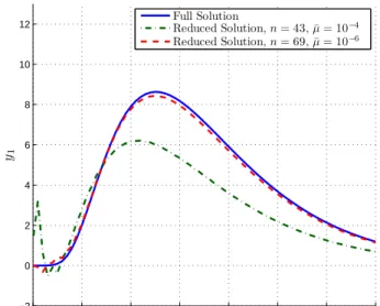
0 0.2 0.4 0.6 0.8 1 1.2 1.4 −2 0 2 4 6 8 10 12 x 10−3 Time y1 Full Solution Reduced Solution,n= 43, ¯µ= 10−4 Reduced Solution,n= 69, ¯µ= 10−6

Figure 4-6: A comparison between full and reduced solutions at sensor location 1 for

two different values of ¯µ. Test initial condition (a) was used to generate the data.

Pe=10, ¯λ = 0.01, two-sensor case. The output at the first sensor location is plotted

here.

the maximum error over all 1000 trials is found to be 0.0059, which is well below the

upper boundεmax= 0.0457 established by (3.21).

Effect of variations in µ¯. As discussed above, ¯µ is the parameter that controls

the number of POD vectors n chosen for inclusion in the reduced basis. If ¯µ is too

large, the reduced basis will not span the space of all initial conditions for which it is

desired that the reduced model be valid. Figure 4-6 illustrates the effect of changing

¯

µ. The curve corresponding to a value of ¯µ = 10−6 _{shows a clear improvement over}

the ¯µ = 10−₄

case. This can also be seen by comparing the errors ε = 0.0229 and

0.0023 associated with the two reduced models seen in Figure 4-6. However, the

improvement comes at a price, since the number of basis vectors, and therefore the

size of the reduced model n, increases from 43 to 69 when ¯µ is decreased.

Effect of variations in λ¯. Another way to alter the size and quality of the reduced

model is to indirectly changep, the number of eigenvectors ofHthat are used as seed

initial conditions for basis creation. We accomplish this by choosing different values of the eigenvalue decay ratio ¯λ. The effect of doing so is illustrated in Figure4-7. An

0 0.2 0.4 0.6 0.8 1 1.2 1.4 −0.005 0 0.005 0.01 0.015 0.02 0.025 0.03 0.035 0.04 Time y2 Full Solution Reduced Solution,n= 62, ¯λ= 0.1 Reduced Solution,n= 128, ¯λ= 0.01

Figure 4-7: Lowering ¯λ to increase p, the number of Hessian eigenvector initial

con-ditions used in basis formation, leads to more accurate reduced-order output. Test

initial condition (c) was used with two output sensors, Pe=100 and ¯µ= 10−4_{. The}

output at the second sensor location is plotted here.

increase in reduced model quality clearly accompanies a decrease in ¯λ. This can also

be seen by comparing rows 1 and 3 of Table4.1, which correspond to the two reduced

models seen in Figure 4-7. The increase in n with lower values of ¯λ is expected,

since greater p implies more snapshot data with which to build the reduced basis,

effectively uncovering more full system modes and decreasing the relative importance

of the most dominant POD vectors. In general, for the same value of ¯µ, more POD

vectors are included in the basis if ¯λ is reduced.

4.1.3

Ten-sensor case

To understand how the proposed method scales with the number of outputs in the

system, we repeat the experiments for systems withQ= 10 outputs corresponding to

sensors in the randomly-generated locations shown in Figure 4-1. A reduced model

was created for the case of Pe=100, with ¯µ = 10−₄

and ¯λ = 0.1. The result was a

reduced system of sizen = 245, which was able to effectively replicate all ten outputs

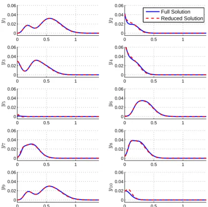
0 0.5 1 0 0.02 0.04 0.06 y1 0 0.5 1 0 0.02 0.04 0.06 y2 0 0.5 1 0 0.02 0.04 0.06 y3 0 0.5 1 0 0.02 0.04 0.06 y4 0 0.5 1 0 0.02 0.04 0.06 y5 0 0.5 1 0 0.02 0.04 0.06 y6 0 0.5 1 0 0.02 0.04 0.06 y7 0 0.5 1 0 0.02 0.04 0.06 y8 0 0.5 1 0 0.02 0.04 0.06 y9 Time 0 0.5 1 0 0.02 0.04 0.06 y1 0 Time Full Solution Reduced Solution

Figure 4-8: A comparison of the full (N = 1860) and reduced (n = 245) outputs for

allQ= 10 locations of interest. Test initial condition (c) was used to generate these

data with Pe = 100, ¯µ= 10−4_{, ¯λ= 0.1.}

model predictions at all ten sensor locations.

The size n = 245 of the reduced model in this case is considerably larger than

that in the corresponding two-output case (n = 62), which is shown in the first row

of Table 4.1, although both models were constructed with identical values of ¯µ and

¯

λ. The difference between high- and low-Q experiments is related to the Hessian

eigenvalue spectrum. As demonstrated in Figure4-2, the eigenvalue decay rate of the

Q= 10 case is less rapid than that of theQ= 2 case. This means that, for the same

value of ¯λ, more seed initial conditions are generally required for systems with more

outputs. Since additional modes of the full system must be captured by the reduced model if the number of sensors is increased, it is not surprising that the size of the reduced basis increases.

4.1.4

Observations and Recommendations

The results above for the 2-D model problem demonstrate that reduced models formed by the proposed methods can be effective in replicating full-scale output quantities of

interest. Algorithm 2 has also been shown to produce models of similar quality and

size as models generated by Algorithm 1. Given also its straightforward

implementa-tion and lower offline cost (since we do not need to form the reduced model at each

greedy iteration), Algorithm 2 is generally preferred for the construction of reduced

bases. At this point, we can use the results to make recommendations about choosing ¯

µand ¯λ, the two parameters that control reduced-model construction.

In practice, one would like to choose these parameters such that both the reduced

model sizenand the modeling error for a variety of test initial conditions are minimal.

The size of the reduced model is important becausen is directly related to the online

computational cost; that is,ndetermines the time needed to compute reduced output

approximations, which is required to be minimal for real-time applications. The offline cost of forming the reduced model is also a function of ¯µand ¯λ. When ¯µis decreased, the basis formation algorithm requires more POD basis vectors to be computed; thus,

decreasing µ increases the offline cost of model construction. In addition, the online

cost of solving the reduced system in (2.12) and (2.13), which is not sparse, scales

with n2_{T. While decreasing ¯µ might appreciably improve modeling accuracy, doing}

so can only increase the time needed to compute reduced output approximations.

Changes in ¯λ affect the offline cost more strongly. Every additional eigenvector of H

to be calculated adds the cost of several additional large-scale system solves: several forward and adjoint solves are needed to find an eigenvector using the matrix-free Lanczos solver described earlier. In addition, the number of columns of the POD

snapshot matrix X grows by (T + 1) if p is incremented by one; computing the POD

basis thus becomes more expensive. If these increases in offline cost can be tolerated, though, the results suggest a clear improvement in reduced-model accuracy for a relatively small increase in online cost.

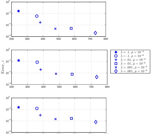
200 300 400 500 600 700 800 10−6 10−4 10−2 100 200 300 400 500 600 700 800 10−6 10−4 10−2 100 E rr o r, ε 200 300 400 500 600 700 800 10−6 10−4 10−2 100

Size of reduced system,n

¯ λ=.1, ¯µ= 10−4 ¯ λ=.1, ¯µ= 10−6 ¯ λ=.01, ¯µ= 10−4 ¯ λ=.01, ¯µ= 10−6 ¯ λ=.001, ¯µ= 10−4 ¯ λ=.001, ¯µ= 10−6

Figure 4-9: A measure of the error in six different reduced models of the same system

plotted versus their sizes n for the ten-sensor case. The three plots were generated

with test initial conditions (a), (b), and (c), respectively. Pe=100, Q= 10 outputs.

parameters ¯µ and ¯λ. For the case of ten output sensors with Pe=100, six different

reduced models were constructed with different combinations of ¯µ and ¯λ. The three

plots in Figure 4-9 show the error ε versus the reduced-model size n for each of the

test initial conditions in Figure4-3. Ideally, a reduced model should have both small

error and smalln, so we prefer those models whose points reside closest to the origin.

Ignoring differences in offline model construction cost, decreasing ¯λ should be favored

over decreasing ¯µif more accuracy is desired. This conclusion is reached by realizing

that for a comparable level of error, reduced models constructed with lower values of ¯

λ are much smaller. Maintaining a small size of the reduced model is important for

4.1.5

Output-Weighted POD Results

To this point, this chapter has presented results computed with the classical POD

described in Section 2.2. In Section 2.3, though, we proposed a method to create

reduced models by weighting snapshots before applying POD. These weights are

dependent on the integral (2.27) of the output norm over time, beginning from the

instant at which each snapshot is taken. The intended result of the output-weighted POD is the construction of reduced bases that require fewer basis vectors than do classical POD bases to provide the same degree of output accuracy. Alternatively, a basis formed with the weighted variant should provide greater accuracy with the same number of basis vectors as a classical POD basis.

To test the weighted method, results were collected for the ten-sensor case with

P e= 100 and ¯λ = 0.01. The parameter ¯µwas adjusted so that two reduced models

with 383 basis vectors were constructed: one via classical POD, and the other using output-weighted POD. When the tight error bounds are compared, the results show a

slight advantage to using the output-weighted POD (εmax = 0.0241) over the classical

POD (εmax = 0.0253). In addition, when both reduced models are subjected to the

same 1000 test initial conditions constructed f