ACOUSTIC SCENE CLASSIFICATION USING DEEP LEARNING-BASED ENSEMBLE
AVERAGING
Jonathan Huang
1, Hong Lu
1, Paulo Lopez-Meyer
2,
Hector A. Cordourier Maruri
2, Juan A. del Hoyo Ontiveros
21
Intel Corp, Intel Labs, 2200 Mission College Blvd.,Santa Clara, CA 95054, USA,
{
jonathan.huang, hong.lu
}
@intel.com
2
Intel Corp, Intel Labs, Av. Del Bosque 1001, Zapopan, JAL, 45019, Mexico,
{
paulo.lopez.meyer, hector.a.cordourier.maruri, juan.antonio.del.hoyo.ontiveros
}
@intel.com
ABSTRACT
In our submission to the DCASE 2019 Task 1a, we have explored the use of four different deep learning based neural networks archi-tectures: Vgg12, ResNet50, AclNet, and AclSincNet. In order to improve performance, these four network architectures were pre-trained with Audioset data, and then fine-tuned over the develop-ment set for the task. The outputs produced by these networks, due to the diversity of feature front-end and of architecture differences, proved to be complementary when fused together. The ensemble of these models’ outputs improved from best single model accuracy of 77.9% to 83.0% on the validation set, trained with the challenge default’s development split. For the challenge’s evaluation set, our best ensemble resulted in 81.3% of classification accuracy.
Index Terms— DCASE, Acoustic Scene Classification, Deep Learning, Neural Networks, Transfer Learning, End-to-End archi-tectures, Ensemble Averaging.
1. INTRODUCTION
In the Detection and Classification of Acoustic Scenes and Events 2019 challenge (DCASE 2019), acoustic data were provided to solve different audio related tasks [1]. Task 1 refers to the challenge of building a model to classify different recordings into predefined classes corresponding to recordings of different environment set-tings in several large European cities.
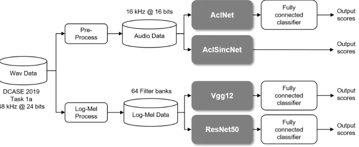
Following the guidelines provided by the challenge in the Task 1 subtask a(Task 1a), we experimented with four different deep learning (DL) neural network architectures: Vgg12, ResNet50, AclNet, and AclSincNet (Figure 1). The Vgg12 and ResNet50 ar-chitectures are adaptations of well-known computer vision CNNs adapted to the audio classification task, with 12 and 50 layers, re-spectively; they both take Mel-filterbank of 64 spectral dimensions as input features. On the other hand, AclNet is an end-to-end (e2e) architecture that takes raw audio input into two layers of 1D CNNs, followed by a VGG-like 2D CNN. AclSincNet is similarly an e2e approach, with the difference in the 1D convolution layers; the 1D convolution layers are essentially combinations of sinc functions, or equivalently band-pass filters, whose cut-off frequencies are the learnable parameters in the model training process.
2. METHODOLOGY
In this section, we describe in detail the experimentation we fol-lowed for our submission to the DCASE 2019 Task1a.
2.1. Data Processing
The DCASE 2019 Task 1a dataset consists of 10-second audio recordings obtained at 10 different acoustic scenes: airport, indoor shopping mall, metro station, pedestrian sreet, public square, street with medium level of traffic, traveling by tram, traveling by bus, traveling by and underground metro, and urban park , recorded at 12 major European cities [2].
The challenge provides as part of this task a 1-fold arrangement for development, i.e. training and validation data splits. In addi-tion to the 1-fold defined, we also experimented with 5-fold random splits over all available data (training/validation), and city held-out validation sets resulting in 10 training/validation splits (only data from 10 cities were available in the development set). Additionally, through the development stage we used Google Audioset data [3] to pre-train all of our implemented DL architectures.
For the development of e2e DL architectures, the two binaural channels were averaged into a single one, and the resulting signal was down sampled from its original 48 kHz to 16 kHz. For the development of spectral based DL architectures, audio data from each channel were processed to generate Mel-filterbank represen-tations with 64 filter bands over a time window of 25 milliseconds and overlaps of 10 milliseconds, resulting in two Log-Mel filterbank channels (Figure 1). Because our early experiments of using mul-tiple channels did not yield improvement over single channel, we opted to use a randomly selected channel in the training process, and channel 0 in the testing.
2.2. Neural Network Architectures
2.2.1. AclNet
AclNet is an e2e CNN architecture, which takes a raw time-domain input waveform as opposed to the more popular technique of us-ing spectral features like Mel-filterbank or Mel-frequency cepstral coefficients (MFCC). One of the advantages of e2e architectures like this is that the front-end feature makes no assumptions of the frequency response. Its feature representation is learned in a data-driven manner, thus its features are optimized for the task at hand as long as there is sufficient training data. We followed the specific settings corresponding to the AclNet work described in [4], with a width multplier of 1.0 and conventional convolutions.
The AclNet architecture we developed for this work was pre-trained with Audioset that resulted in 527 outputs, which in turn were used as embeddings to train a fully-connected layer classifier with ReLU activation functions in a transfer learning manner. Raw
Figure 1: Development of our proposed deep learning architectures for audio scene classification in the DCASE 2019 Task 1a. audio data at 16 kHz form the DCASE 2019 challenge was fed to
the pre-trained AclNet, and embeddings were used to train the clas-sifier.
We performed a search for the optimal parameters of this DL model. We experimented with different values and configurations, and ended with the best performing model when using the hyper parameters described in Table 2; cosine annealing for the learning rate schedule, and the use of mixup for data augmentation [5] were considered, but it was observed that they did not improve the clas-sification performance. During the training, 1-second of audio was randomly selected from mini-batches of 64 training clips. At test time, we run the inference on 1-second non-overlapping consecu-tive audio segments, and then average the outputs over the length of the test audio. The experimental results obtained by this e2e archi-tecture can be seen in Table 3.
2.2.2. AclSincNet
The AclSincNet architecture consists of two building blocks of the network: a low-level Spectral like features (SLF), and a high-level features (HLF).
The SLF is a set of features designed to be similar to the spectral features used in conventional audio processing. It can be viewed as a replacement of the spectral feature, but it is fully differentiable and can be trained with backward propagation. The front-end is inspired by SincNet [6]. We used the same setup as suggested in the original work but with a stride length of 16 milliseconds; the authors of SincNet treat the output of the SincNet layer as a replacement of the FFT filter bank, and feed it directly into the subsequent CNN layer. We took a different route, aiming to replicate the output of Mel-filterbank calculation more closely. We first compute the square of the output before average pooling over multiple time steps, and then follow up by the log operation to make the filterbank output less sensitive to amplitude variations. With the time-domain waveform as input, the SLF layer produces an output of 256 channels at feature frame rate of 10 milliseconds after the average pool layer. In our setup, a 1.280-second input produces an output tensor of dimension (256, 1, 128).
Taking the output from the SLF block, the high level feature
Table 1: SLF Architecture used in AclSincNet
Layer Description
Sincnet1D kernel size 251, stride length 16 BatchNorm
Calculate energy spectrum x = x2
Average pooling 100ms window with 50ms stride Clamp the min x = x.clamp(min=1e-12) Calculate log() x = log(x)
layer treats it as a 2D image (e.g. a 256x128 image for the 1.28-second input) and applies standard VGG-like 2D CNN. The archi-tecture of the HLF is similar to typical image classification CNNs. We experimented with a number of different architectures, and found that a VGG-like architecture provides good classification per-formance and well-understood building blocks. In our case, each of the conv layers are a standard building block that comprises a 2D convolution layer, batch normalization, and PReLU activation.
We did not use fully connected layers as in standard VGG; in-stead, we simply apply average pooling to output the scores. The final layers of the AclSincNet is a 1x1 convolution that reduces the number of channels to the number of classes (10 classes in the DCASE 2019 challenge). Before the input to the 1x1 convolution layer, we add a dropout layer for regularization. We found a dropout probability of 0.9 to work well on this task. Each of the 10 chan-nels are then average pooled and output directly after SoftMax. The advantage of these final two layers is that our architecture can incor-porate arbitrary length inputs for both training and testing, without any need to modify the number of hidden units of a the fully con-nected layers.
We pre-trained this model with AudioSet [3] and then fine tuned it with the DCASE 2019 Task 1a data. During fine-tuning, we use 6-seconds audio data (random crop from each of the 10-second sam-ple) for training, and 10-second data (the complete clip) for testing. We experimented with different number of layers, number of chan-nels, and kernel size on the data set. While the total number of the parameter is rather big (Table 3), we noticed that the network scales quite well when we shrink the layer, channel, and kernel size. We
observed experimentally that the accuracy only drops 1 to 2% when a network with 18M parameters is used. However, we decided to stick to the larger network for this challenge.
2.2.3. Vgg12
The Vgg12 model is an adaptation of the well-known VGG archi-tecture [7]. It has a total of 12 convolutional layers, with the first one having 64 channel output, and the last one 512 outputs. At the output of each conv layer, we apply batch normalization followed by ReLU activation. Through the conv layers, there are 5 max-pool layers with kernel size of 2. A key architectural difference is that the network is designed for variable input size (e.g. 64 spectral di-mensions and arbitrary number of time steps). The output of the last convolutional layer is average pooled, to always produce a vec-tor length of 512 values. This vecvec-tor is then followed up by a fully connected layer to produce the 10-class output defined by the chal-lenge.
During the training phase, 5-seconds of audio are randomly se-lected from the training clip. At test time, we run the inference on 1-second non-overlapping segments, and then average the outputs over the length of the test audio.
2.2.4. ResNet50
Our audio ResNet50 has exactly the same convolutional layers as the architecture in the original ResNet paper [8]. Again, we made the same adaptations as in Vgg12 described in 2.2.3, to take a variable length input Mel-filterbank spectra into a single 10-class output. We also used the training and testing sequence selection scheme applied for the Vgg12.
During the training, we used SpecAugment [9] as a data aug-mentation scheme. This data augaug-mentation works by masking out random time and spectral bands of randomly selected width. We opted to mask only spectral bands, at random positions with width uniformly sampled from [0, 20] Mel bands. We found that this aug-mentation gave a 1% improvement over the same network without SpecAugment.
2.3. Training Strategy
In addition to the default train/validation split provided by DCASE 2019 Task 1a, we used two strategies to train our models for score averaging: 5-fold cross-validation and leave-one-city-out cross val-idation. In both cases, we merged the development and validation data set together and re-split all the labelled data set with the above two strategies to train models accordingly.
With the 5-fold cross-validation method, all the labelled data were split into 5 folds with random shuffle, i.e. 4/5 of the data set is used for training and 1/5 of the data set is used as validation set. Five models are trained and their scores are averaged as the final score. i.e. the final output is essentially the ensemble average of 5 individually trained models.
Similarly, the leave-one-city-out method was done in the same way with a different split methodology. Instead of random split, the split is done by city. i.e. 9 cities are used for training and 1 city is held out and used as the validation set. Therefore, 10 models are trained and their scores are averaged as the final output.
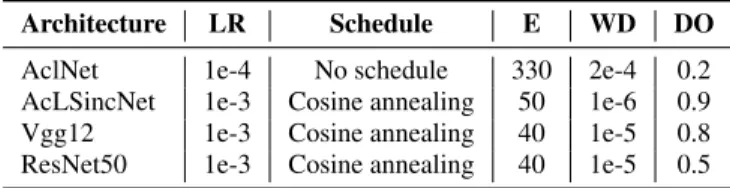
All four architectures were trained with the Adam optimizer. The training hyper parameters (learning rate LR, LR schedule, num-ber of epochs E, drop out rate DO, and weight decay WD) of each of the architectures are listed in Table 2. During the fine-tuning
Table 2: Training setup values for the four deep learning architec-tures proposed. The values displayed are the learning rate, learning rate schedule, number of epochs, weight decay, and drop out rate, respectively.
Architecture LR Schedule E WD DO AclNet 1e-4 No schedule 330 2e-4 0.2 AcLSincNet 1e-3 Cosine annealing 50 1e-6 0.9 Vgg12 1e-3 Cosine annealing 40 1e-5 0.8 ResNet50 1e-3 Cosine annealing 40 1e-5 0.5 Table 3: Classification results over the validation set obtained by the individual deep learning based neural network architectures ex-plored in this work.
Architecture Params Accuracy AclNet 19.3M 0.7481 AclSincNet 52.2M 0.7608 Vgg12 12.8M 0.7744 ResNet50 24.5M 0.7787
process, we kept the part of the corresponding Audioset pre-trained network with a LR value that is 1/10th of the LR as the rest of the network. The validation set were used for model selection, i.e. the best performing model on the validation set were saved and used for inference.
2.4. Ensemble Averaging
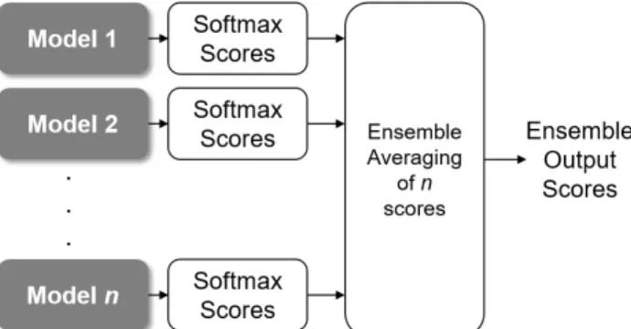
In order to reduce individual variance of each of the developed DL models described in the previous subsections, we applied ensemble averaging technique, which is one of the simplest ensemble learning methodologies used in machine learning to improve the prediction performance [10]. This approach consists on the averaging of the prediction scores obtained by different models, as seen in Figure 2. By combining the prediction scores from different DL models that performed above the reported challenge baseline, the intention is to add a bias that counters the variance of a single trained model. Having a diversity of DL models helps to achieve this intention. In our experiments, we have extensively explored different combina-tion sets of our DL models in order to find the ones that better gen-eralize over the validation data set. Experimental results obtained for some of the most obvious combinations are shown in the next section.
3. RESULTS
The experimental results obtained for our developed DL models over the validation data set are shown in Table 3. These are the best experimental validation accuracy results achieved by our individu-ally trained DL models at the time of the DCASE 2019 submission deadline. For each one of the developed models, the number of trainable parameters is listed also in Table 3 to present an idea of the size of the DL architectures used.
In Table 4, the results from the best combinations of two, three, and four DL models that were obtained through ensemble averaging of their output scores. All outputs were defined as softmax scores in order to have compatible values for averaging across the ensemble. It can be observed how the experimental results over the validation set yield into higher accuracy (Table 4) when compared to
individ-Table 4: Classification results over the validation set obtained from the ensemble averaging combination of two, three, and four deep learning based neural networks architectures.
Architecture Params Accuracy
AclSincNet+ResNet50 76.8M 0.8127 Vgg12+AclSincNet+ResNet50 89.7M 0.8184 AclNet+Vgg12+AclSincNet+ResNet50 109.0M 0.8301 ual models results (Table 3). These results support the idea that utilizing the combination of predictions from different DL models results in a reduction of variance, and in more accurate predictions [10].
For our four allowed submissions to DCASE 2019 Task 1a, we experimented with the DL architectures described above, developed with different types of data splits, and combining their output pre-dictions through ensemble averaging. In the next section we pro-vide a detailed description of the combinations used as part of our complete final submission.
4. SUBMISSIONS TO DCASE 2019 TASK 1A Our four submissions to the DCASE 2019 Task 1a consists of the ensemble averaging of different predicted scores from different DL architectures. Below is a detailed description list of the ensemble models used to generate the submission labels on the evaluation data set provided:
1. Ensemble averaging obtained from a combination of 40 individ-ually trained DL architectures: 1 Vgg12, trained with the default data split defined by the challenge; 10 Vgg12, each trained with 1 of the 10 leave-one-city-out splits; 5 AclSincNet, trained with 5 different random splits; 10 AclSincNet, each trained with 1 of the 10 leave-one-city-out splits; 3 Resnet50, each trained with three different data splits; 10 ResNet50, each trained with 1 of the leave-one-city-out splits; and 1 AclNet, trained with the de-fault data split defined by the challenge. Considering each one of the 40 DL architectures combined, the total number of trainable parameters resulted in 1,264.4M.
2. Ensemble averaging obtained from a combination of 31 in-dividually trained DL architectures: 10 Vgg12, each trained with 1 of the 10 leave-one-city-out splits; 10 AclSincNet, each trained with 1 of the 10 leave-one-city-out splits; 10 ResNet50, each trained with 1 of the 10 leave-one-city-out splits; and 1
Figure 2: Ensemble averaging of n independently trained deep learning models.
Table 5: Classification results over the evaluation set obtained from four different ensemble averaging combinations of deep learning architectures, submitted to the DCASE 2019 challenge Task 1a.
Architecture Params Accuracy Challenge Rank Ensemble 1 1,264.4M 0.8050 15 Ensemble 2 921.7M 0.8110 12 Ensemble 3 798.6M 0.8130 10 Ensemble 4 374.7M 0.7950 22
Resnet50, trained with 1 data split. Considering each one of the 31 DL architectures combined, the total number of trainable pa-rameters resulted in 921.7M.
3. Ensemble averaging obtained from a combination of 26 individ-ually trained DL architectures: 10 Vgg12, each trained with 1 of the 10 leave-one-city-out splits; 5 AclSincNet, trained with 5 different random splits; 10 ResNet50, each trained with 1 of the 10 leave-one-city-out splits; and 1 Resnet50, trained with 1 data split. Considering each one of the 26 DL architectures combined, the total number of trainable parameters resulted in 798.6M.
4. Ensemble averaging obtained from a combination of 20 individ-ually trained DL architectures: 10 Vgg12, each trained with 1 of the 10 leave-one-city-out splits; and 10 ResNet50, each trained with 1 of the 10 leave-one-city-out splits. Considering each one of the 20 DL architectures combined, the total number of train-able parameters resulted in 374.7M.
The final Task 1a challenge results obtained from these four en-sembles over the evaluation set are shown in Table 5. The best result obtained of 81.3% ranked 10th across all submissions, and 5th by team submissions. Our submission consisted on simple ensemble averaging; part of our ongoing efforts consists of exploring other ensemble methodologies, e.g. stacking, to increase the predictive force of the classifiers.
5. CONCLUSIONS
Starting from individually trained DL models, we were able to achieve above the baseline results as reported in the DCASE 2019 Task 1a challenge. From these, we were able to increase the perfor-mance of the audio scene classification by combining the prediction scores of different DL models through ensemble averaging. By do-ing this ensemble, we obtained significantly higher classification results over the validation set than the ones obtained by individual DL models, i.e. 83.0%Vs77.9% , respectively. Our best ensemble model resulted in a 81.3% classification accuracy over the evalua-tion set provided by the challenge.
6. REFERENCES
[1] Detection and Classification of Acoustic Scenes and Events Challenge 2019. http://dcase.community/ challenge2019.
[2] Heittola, Toni; Mesaros, Annamari; Virtanen, Tuomas. ”TAU Urban Acoustic Scenes 2019, Development dataset”,Zenodo, 2019.http://doi.org/10.5281/zenodo.2589280 [3] Gemmeke, Joft F.; Ellis, Daniel P. W.; Freedman,
Plakal, Manoj; Ritter, Marvin. ’Audio Set: and Ontol-ogy and human-Labeld Dataset for Audio Events”,ICASSP, 2017. https://ieeexplore.ieee.org/abstract/ document/7952261.
[4] Huang, Jonathan; Alvarado-Leanos, Juan. ”AclNet: efficient end-to-end audio classification CNN”,CoRR, 2018.http: //arxiv.org/abs/1811.06669
[5] Zhang, Hongyi; Cisse, Moustapha; Dauphin, Yann N.; Lopez-Paz, David. ”mixup: Beyond Empirical Risk Minimization”,
arXiv:1710.09412 [cs.LG], 2018. https://arxiv.org/
abs/1710.09412
[6] Ravanelli, Mirco; Bengio, Yoshua. ”Speaker Recognition from Raw Waveform with SincNet”,CVPR, 2018.https: //arxiv.org/abs/1808.00158
[7] Simonyan, Karen; Zisserman, Andrew. ”Very Deep
Convolu-tional Networks for Large-Scale Image Recognition”,ICLR, 2015.https://arxiv.org/abs/1409.1556
[8] He, Kaiming; Zhang, Xiagyu; Ren, Shaoqing; Sun, Jian. ”Deep Residual Learning for Image Recognition”, CVPR, 2019.https://arxiv.org/abs/1512.03385 [9] Park, Daniel S.; Chan, William; Zhang, Yu; Chiu,
Chung-Cheng; Zoph, Barret; Cubuk, Ekin D.; Le, Quoc V.. ”Specaugment: A simple data augmentation method for au-tomatic speech recognition”, arXiv:1904.08779 [eess.AS], 2019.https://arxiv.org/abs/1904.08779 [10] Brownlee, Jason. ”Ensemble Learning Methods for Deep
Learning Neural Networks”, Machine Learning Mastery!, 2018. https://machinelearningmastery.com/ ensemble-methods-for-deep-learning-neural-networks