Do Stock Markets move together?

(1)

(Unpublished)

Access from the University of Nottingham repository:

http://eprints.nottingham.ac.uk/25665/1/Do_Stock_Markets_Move_Together.pdf

Copyright and reuse:

The Nottingham ePrints service makes this work by researchers of the University of Nottingham available open access under the following conditions.

· Copyright and all moral rights to the version of the paper presented here belong to the individual author(s) and/or other copyright owners.

· To the extent reasonable and practicable the material made available in Nottingham ePrints has been checked for eligibility before being made available.

· Copies of full items can be used for personal research or study, educational, or not-for-profit purposes without prior permission or charge provided that the authors, title and full bibliographic details are credited, a hyperlink and/or URL is given for the original metadata page and the content is not changed in any way.

· Quotations or similar reproductions must be sufficiently acknowledged.

Please see our full end user licence at:

http://eprints.nottingham.ac.uk/end_user_agreement.pdf A note on versions:

The version presented here may differ from the published version or from the version of record. If you wish to cite this item you are advised to consult the publisher’s version. Please see the repository url above for details on accessing the published version and note that access may require a subscription.

(2)

NIANLONG XU

(3)

University of Nottingham

Do Stock Markets Move Together?

Presented by

NIANLONG XU

Academic Year 2012

A dissertation presented in part consideration for the degree of

MSc Finance and Investment

(4)

Abstract

In this paper, the purpose of this dissertation is to analyze the co-movements among Chinese, Hong Kong, the United States and Japanese stock market.

This dissertation provides evidences to support the hypothesis that there may be long-term benefits for Chinese investors to diversify in the international equity markets. The evidences are based on the data from the stock markets of the United States, Hong Kong, China and Japan over the period of 1st January 2007 to 31st December 2011. Time- series analytical techniques are applied including Granger Causality test and the Vector auto-regression (VAR) model.

It is found that the stock markets of both Hong Kong and Japan significantly influence on the Chinese stock market while the United States stock market doesn’t. The correlation between Chinese stock market and the United States stock market is found not strong. However, the results indicate that the impacts from Hong Kong stock market and Japanese stock market on Chinese stock market fade quickly and may not be last in the long run. The results also suggest Japanese stock market has little impact on Chinese stock market compared to Hong Kong. Furthermore, such co-movements phenomenon between the Chinese stock market and the international markets may exist, but not persist in long term. In one word, Chinese stock market seems move together with Hong Kong and Japanese stock market in short term. Therefore, the study suggests that, for Chinese investors’ considerations, it is benefit to diversify across international equity markets. The findings could be contributed reference for Chinese investors who attempt to apply an international diversification strategy while constructing their portfolios.

(5)

Acknowledgements

I would like to thank all those who supported and helped me to complete this dissertation and my master degree. I wish to extend the highest gratitude to my supervisor Professor Bob Berry, who indeed provides me a lot of finance knowledge and encourages me to face the challenges.

I also would like to dedicate this dissertation to my mother, who has given me her unconditional support and love, which inspired me throughout the one-year study at the University of Nottingham.

Finally, I am very grateful to all my dear friends and lovely girlfriend Xiaochen Li that have made this an enjoyable and meaningful year.

(8)

Chapter 1 Introduction

1.1 Research Motivation

Many studies have shown that the world capital markets are becoming more integrated and that major financial markets share increased co-movements (Allen and Macdonald, 1995). The explainable reason for this trend might be the financial deregulation in many emerging countries, and technological developments that provide unlimited speed of information transmission, as well as the expansion of multinational enterprises. Such globalisation phenomenon in financial world have improved ties between national stock markets and increased the co-movement behaviours of international stock markets. This co-movement of behaviour draws attention from academic community, and is especially important to gain benefit through international diversification. In recent decades, lots of studies focus on studying the correlations among international stock markets in order to gain idea of beneficial effects of international diversification strategies.

Chinese stock market has developed rapidly, especially in recent years. By 2002, the total market capitalization of SHSE was US$ 2.38 trillion. In 2007, the total market capitalization of SHSE was US$ 26.98 trillion. Having entered the World Trade Organization (WTO), China has further opened its capital markets (Shanghai Stock Exchange, 2007).

Here come the concerns: Does the Chinese stock market move together with international stock markets? And, is it possible to diversify the risk of portfolio for Chinese investors to construct international portfolio.

(9)

Studying the co-movements of international stock markets has long been a popular research topic in finance. Low correlation between national stock markets is often presented as evidence in support of the benefit of global portfolio diversification (Levy and Sarnat, 1970; Solnik, 1974). Several studies investigated the co-movements of national stock markets in a given geographical. For example, Friedman and Shachmurove (1997) and Mercic and Meric (1997) showed that the correlation between the European stock markets had been increasing and the portfolio diversification benefit with these stock markets had been decreasing. Ng (2002) studied the co-movements of Asian stock markets. Although the co-movements of the stock markets in different regions of the world had been studied extensively, the co-movements between Chinese stock market and the other national stock markets had not received sufficient attention.

Therefore, the objective of this paper is addressed to investigate the co-movements between Chinese stock market and the other national stock markets. Hopefully, the findings can support the view that it is benefit for Chinese investors through constructing international portfolio, and further to help Chinese investors to have a better understanding of co-movement of the Chinese stock market and international stock markets. The brief purpose of this study is offering a reference for Chinese investors and international investors to evaluate the desirability of international diversification. The exploration of correlations between the Chinese stock market and the other national stock markets may allow Chinese investors to gain some knowledge of efficiency of investment through international diversification and how to construct a possible international diversified portfolio.

In order to investigate the co-movement phenomenon between the Chinese stock market and the international stock markets, the inter-covariance and the correlation coefficient will be examined. Although there have been much previous research regarding the correlations

(10)

among international stock markets carries out, but with limited literatures focus on the Chinese stock market. Even worse, many of these have failed to involve the time-varying property. Moreover, the correlation coefficient values may not provide the further relationship among international stock markets. Therefore, in this paper, some time-series statistical techniques are applied in order to analyse the co-movement of international stock market.

After test the correlation coefficient, the cause and effect relationship can be tested by addressing the Granger Causality test. An Impulse Response analyse will be utilized to examine the response of Chinese stock market to the fluctuations of the other national stock markets.

In one word, the motive of this study is to investigate that whether the Chinese stock market move together with international stock markets or not, which including the United States, Japanese and Hong Kong stock market.

As far as readers know, the paper is the first to systematically analyze the co-movement between Chinese stock market and the other three national stock markets during the period of 2007 to 2011 which is recognised as financial crisis period. The test results in this paper can help Chinese individual investors and institutional investors gain benefits from an international diversification strategy during this period. Meanwhile, the paper may indicate some changing economic phenomenon. For example, the study may answer these questions: Is the United States equity market still leading the world financial markets during the world financial crisis period? Which national equity market affects Chinese stock market most significantly?

The paper is structured as follows. The next section presents a literature review on the co-movements among the international stock markets. Chapter 3 describes the methodologies to

(11)

investigate the co-movements among international stock markets. Chapter 4 continues with an analysis of the co-movements among international stock markets, more prone on how the other national stock markets influence Chinese stock market. Chapter 5 discusses the results analysis and illustrates findings of this paper, follows with the contributions and limitations sections.

Chapter2 Literature review

Some scholars have researched on the linkages among national stock markets. Due to the different methodologies and utilized data, the results they got are usually significantly different from each other. Lots of studies focus on the linkage among developed countries, but few on developing countries.

It is crucial to review the background of the research, as well as the sounded methodologies before carrying out the research. Under the considerations, some essential literature is compiled and summarised; the logic used to sort this literature is described by the following three parts, respectively: (1), as regards our research question and motivation, the international diversification strategy literatures in the investment field will be summarised; (2), in order to highlight the research background and methodologies applied for the research question, literatures about correlations among international stock markets will be compiled to provide the knowledge support; (3), last, follows the discussion regarding the time series analysis techniques.

2.1 The Benefit of International Diversification

The possibility of the international portfolio had long been a tradition in many countries. According to Solnik and Mcleavey (2004), there was a strong trend toward international diversification in all countries. In the early 1970s, U.S. pension funds held no foreign assets;

(12)

the percentage of foreign assets was increased to 15 percent of total assets by 2000. British institutional investors hold more than 25 percent of their assets invested abroad. Some Dutch pention funds have more than half of their assets invested abroad. Recently, private investors have joined international investment group.

In 1974, the New York Stock Exchange was the only significant market in the world, representing 60 percent of a world stock market capitalization. The share of the United States moved from 60 percent to less than 30 percent in 1988. In 2001, the share of the United States was 50 percent, the share of European makes up one-third of world capital market, while the share of Asian made up one-sixth of world stock market capitalization. In August 2006, China had just the 15th largest equity market in the world. Today, China ranks second ahead of Japan, the UK and Hong Kong. This indicates that there are some potential benefits to invest in other countries which developed very fast, hence, international diversification could be applied by investors (Solnik and Mcleavey, 2004).

The advantage of international diversification is that foreign investments allow investors reduce the total risk of the portfolio, while offering the potential benefits. Solnik and Mcleavey (2004) stated that domestic securities tend to move up or down together because they were similarly affected by domestic conditions, such as monetary announcements, movements in interest rates, budget deficits, and national growth. It created the positive correlation among nearly all stocks traded in the same country. So it is efficient to spread risks and diversify away the national markets risk by international portfolio investment.

2.2 Correlation among international stock market

Markowitz (1952) and Tobin (1952) were first people who introduced the theoretical models of portfolio selection that diversification of risky assets had positive and normative effect.

(13)

Markowitz (1952) indicated that it was obvious to consider not only return but also risk when investors were making decision. While holding different kinds of portfolio, investors may reduce the risk of the portfolio. Markowitz (1952) first came up the idea of constructing of international portfolio could be beneficial. After that, many researches were carried out on international portfolio issue and amount of research methods have been developed in the last few decades.

Grubel (1968) found huge diversification benefit through studying stock market index among eleven countries. In the research of Grubel (1968), a typical investor in the New York Stock Exchange, could increase 68 percentage annual return if the investor invested in the international market, while keeping risk constant. This empirical result showed that international portfolio diversification was more profitable than only invest in one country. More significant, Grubel (1968) indicated that the investor could gain more profit if the correlation coefficient between countries was small. In another word, small correlation coefficient, more significant the beneficial effect of international portfolio diversification.

Solnik (1974) carried out the research on eight countries including United States, United Kingdon, Germany, France, Switzerland, Italy, Belgium and Finland from 1996 to 1997. The purpose of the article was to prove the portfolio diversification in foreign securities had lower risk compared to domestic common stocks. Solnik (1974) demonstrated that the total risk of a portfolio depended not only on the number of securities included in the portfolio but also on the degree of correlation of each riskiness of each individual security. Moreover, Solnik (1974) provided the evidence that international portfolio diversification could efficient hedge the domestic currency devaluation.

There are some researches that focused on the desirability of international diversification strategy for Chinese investors, specifically for Taiwanese investors. Chan, Gup and Pan

(14)

(1992) examined the relationships between four major Asian stock markets including Hong Kong, South Korea, Singapore, Taiwan and the United States. They found that there was not cointegration relationship between four Asian stock markets and the United States market individually or collectively. Therefore, the result indicated that the international diversification strategy was effective for both Asian investors and the United States investors. International diversification is not only successful strategy for stock investment but also expand to bond market investment. In order to prove bonds assets take in account could reduce the risk of international portfolio, Levy and Lerman (1988) conducted a research by collecting data from bond and stock markets of thirteen countries form 1960 and 1980. The empirical results indicated that the portfolio includes stocks and bonds had potential benefits than portfolio that only include stocks. Since, there was substantial benefits by taking bond diversification into account when construct a portfolio.

There might be long run benefit for Chinese investors to construct international portfolio. Sarno (2008) stated that the benefits of international diversification arise from the relatively low level of correlation among national equity market. International portfolio diversification was advocated as a much more efficient way than only domestic investment. Jang and Sul (2002) found that the Chinese market was not integrated with other countries. For Chinese investors, this may be good news, since it implies there exists a long-run benefit existed in international diversification obtained by investment in these countries. The findings may also have provided valuable information to global investors intended to construct a portfolio in which China concluded.

There are lots of studies investigating relationships of stock market among developed countries such as United States, Japan and Europe. Because of the United States is a major investor in many countries and posing a huge political influence on several countries in the

(15)

world, many studies have been done to investigate the causal relationship between the United States and other stock markets. Eun and Shim (1989) examined nine major developed stock markets including Australia, Canada, France, Germany, Hong Kong, Japan, Switzerland, the United Kingdom and the United States from 1979 to 1985, the empirical results indicated that the United States market was leading worldwide trend.

In recent years, many studies have focused on the desirability of diversification strategy for Asian investors. Cheung and Mak (1992) investigated the causal relationship between developed markets and Asian emerging markets and found that United States markets lead both developed and most of developing markets. Masih and Masih (1997) investigated the co-movement between Asian Four Little Dragons and four developed stock markets including Germany, Japan, UK and the U.S. The results indicated that there were significant linkages among these Asian countries. Ghosh, Saidi and Johnson (1999) carried out the research by addressing the question: “Who moves the Asia-Pacific stock markets-US or Japan?” The findings indicated that Hong Kong, India, Malaysia and South Korea are closely correlated with the U.S. market while Indonesia, Philippines, and Singapore much more correlated with Japan. This could be explained by there was strong economic relationship among Hong Kong, India, Malaysia and South Korea. Also there was strong business tie among Indonesia, Philippines, and Singapore. More specifically, for Chinese stock market, Longin and Solnik (1995) stated that correlations tended to increase in times of large shocks to returns such as a stock market crash. Zhu (2004) rejected causal relationship and cointegration between market returns in Shanghai, Shenzhen and Hong Kong; Groenewold (2004) supported cointegration between Shanghai and Shenzhen, but rejected it between mainland markets and Hong Kong and Taiwan. Zhang (2009) found weak return linkage between Shanghai and Hong Kong. Chow and Lawler (2003) found no correlation between Shanghai and New York stock returns and negative correlation between their volatilities,

(16)

using weekly data from 1992 to 2002. They described the negative correlation in volatility as spurious, driven by macroeconomic fundamentals in the United States and China as indicated by a negative correlation between the rates of change in their GDP while their capital markets were not integrated. Li (2007) found evidence of no cointegration between Hong Kong and China’s stock market with multivariate GARCH using daily data from January 2000 to August 2005.

Generally, these literatures given above based on the assumption that diversification can be applied in the international stock market. The returns of some international stock markets were low–correlated, and country factor played a significant role in explaining the returns. Therefore, the benefit can be achieved by constructing international portfolio. This might be explained by the international capital market was a segment market so that investors could diversify country risk and obtained benefits from the reduction of total risk. However, some people said that international markets might not have been low–correlated as these researchers assumed. Campell and Hamao (1992) stated that globalization might drive economic activities across boarders and reduce the barrier. Masih and Masih (1997) argued that the world capital markets were likely become more integrated and that co-movement of international market were increased. This integrated phenomenon might due to the globalization effect.

Additionally, there were also some arguments against the international diversification. Real effect issue was debated that would change the benefits international diversification. There might be some other factors would affect the result when investors make international portfolio. If the real effect was not significant enough for investors to gain benefits efficiently compared with the costs spent in achieving international diversification strategies. The idea

(17)

of international diversification may not be desirable investment strategy. There were many risks regarding international portfolio diversification, one risk is currency exchange risk. Overall, the literature related to international diversification strategies supports the hypothesis that it is beneficial and efficient to diversify risks through international investing. Moreover, many studies that focused on Asian or Chinese stock market specifically indicated that international diversification benefits do exist for Chinese investors. Since the level of effect of diversification benefits depends on the correlation among national markets, therefore, the literature relevant to the correlation among international markets is summarised below in order to provide more profound knowledge about study.

International equity market correlation has been widely studied. The benefits of international portfolio diversification depend on the level of international stock market correlations. There is no doubt that correlation coefficients between two stock markets will change regarding to the changing of country factor. Economic and financial integration between countries could indicate time-varying international correlation coefficients, therefore, increased economic and financial integration between countries leads higher international stock market correlation. Grubel (1968) claimed that correlations were generally lower between international than domestic markets. Grubel and Fadner (1971) investigated the relationships among international stock markets by examining the correlation coefficient matrix. The results indicated that there was low correlation between U.S. and other countries. Grubel and Fadner (1971) believed that other countries had their own business cycle and those countries’ economy was only affected by their man-made shocks. Therefore, there was benefit for United State investors to diversify their risks by investing in the other countries.

However, Ibbotson, Carr, and Robinson (1982) examined the correlation coefficient matrix to test the relationships among international stock market in the world from 1960 to 1980. The

(18)

result was different with Grubel and Fadner (1971). Ibbotson, Carr, and Robinson (1982) found that some national markets had co-movement phenomenon to some other countries, they believed that the returns of some national stock markets were highly related specifically with some other markets.

For instance, Germany, Switzerland, and Holland were highly correlated while the United States, Canada, Australia, Hong Kong and Singapore were correlated. The results suggested the growing trend of information-transfer among countries and the flow of international capital investments lead that the integration and correlation among national stock market increased. Later, Eun and Shim (1989) investigated the international transmission mechanism of stock market movements by estimating a nine-stock market vector auto-regression (VAR) system. The results indicated that the U.S. stock market was the most influential market in the world. No national stock market was nearly as influential as the U.S in terms of its capability of accounting for the error variances of other markets. This finds suggested that the dominant position of U.S. in the world economy.

Koch and Koch (1991) used the dynamic simultaneous equation model to examine the changes of trend of interdependence of eight national stock markets in 1972, 1980 and 1987. The empirical results revealed that over time, the level of interdependence among markets that were within the same geographical regions grew higher. Koch and Koch (1991) found that the responses that from national stock markets to changing of other national stock markets were getting faster. Koch and Koch (1991) also indicated that Japan had more power that influence world stock market after 1972, while United States had smaller power.

Coeurdacier and Guibaud (2009) proved that investors should use foreign stocks to hedge against their domestic risk, for instance, holding frictions constant, it is efficient for investors to invest in foreign equities that have low correlation with their domestic stock market.

(19)

However, these literatures may fail to explain the time varying property of conditional and unconditional covariance of the asset returns. Therefore, the volatilities and correlations estimation models are discussed as follow.

Bollerslev, Chou and Koner (1992) stated that correlation coefficient could not represent the relationship among variables appropriately if the covariance among variables varies in time process. This indicated that correlation coefficient analysis method is not efficient enough to measure the correlation among national stock markets. For instance, an unusual conditional correlation coefficient may cause different results. Thereby, time varying property of the conditional variance has to be taken into account.

In order to test the time varying property of the conditional covariance, a test conducted by King, Sentana and Wadhwani (1994) to examine the covariance across stock markets and evaluate the capital market integration. In the research, King, Sentana and Wadhwani (1994) argued that there was no increased trend of correlation among countries. Generalised autoregressive conditional heteroskedasticity (GARCH) model was applied in the research, the results showed that only a small proportion of covariance between markets could be explained by “observable” economic factors. Therefore, the covariance analyse could not explain the degree of the integration phenomenon among international stock markets efficiently. Login and Solnik (1995) studied the correlation of monthly excess returns of seven national stock markets from 1960 to 1990 by using a multivariate generalised autoregressive conditional heteroskedasticity (1, 1) model. Despite the test result indicated that there was no constant conditional correlation among national stock markets, Login and Solnik (1995) adopted a conditional variance model to capture the evolution in the conditional covariance structure and analysed the independence of the international stock market. The empirical result suggested that the correlation rose within the research period and

(20)

the correlation level increased with volatility, which indicated that the correlation among stock markets might be higher when there is some shock occurred.

Darbar and Deb (1997) carried out research to study the co-movement among four major national markets including United States, Japan, Canada and United Kingdom. The GARCH model was applied in the research. Darbar and Deb (1997) assumed conditional variance consisted two parts: the historical mean covariance and the transitory conditional covariance. They found that all the markets were both permanently and transitorily correlated except for the United States and Japan, which were only transitorily correlated but only correlated in short-term. Furthermore, Darbar and Deb (1997) examined the changes in the correlation pattern among markets by taking the shock in the global stock market in 1989 October into account. The results indicated that the conditional covariance varied with the volatility of the stock market and that it took about three to five days to reflect the shocks and for returning to the permanent level. This study gave the negative signal that international diversification is beneficial if the portfolio was adjusted correctly according to the variations exhibited in the correlations.

2.3 Time Series Analysis Techniques

In the last two decades, time series analysis techniques are applied to examine the phenomenon of co-movement among stock markets. Since the stock market data is a time series dataset, the time process property techniques is suitable to examine the co-movement among stock markets. Therefore, the application of time-series methodology is more appropriate to investigate relationship of stock markets.

Vector autoregressive model (VAR) was applied by Eun and Shim (1989) to investigate the transmission effect among nine national markets. In the research, Eun and Shim (1989) used

(21)

the daily stock market returns of nine national markets. The empirical results indicated that the United States market influenced other national markets most while other national markets did not. This meant that the correlation between the United States stock market and other national markets was significant. Eun and Shim (1989) also found that the other countries responses did not last longer than one day when the shock from the United States. This indicated that the international market was quite information efficient since the innovation effect from the United States was usually quickly absorbed.

Chowdhury (1994) argued that there was an increased trend of integration among national stock markets in the world, Vector auto-regression model (VAR) is applied to investigate the interrelationship among Hong Kong, Singapore, Korea and Taiwan by Chowdhury (1994). The text results suggested that there was a significant correlation between Hong Kong stock market and Singapore stock markets. Furthermore, Chowdhury (1994) also found that the cross-country restriction in investment restrained the response of countries to innovations from other countries. For instance, the markets with strict restrictions on cross-country investment, such as Korea and Taiwan, did not respond to innovations from foreign markets. Moreover, the United States stock market affected the four Asian stock markets while these Asian markets did not influence the United States Stock markets.

Gerrits and Yuce (1999) introduced Granger Causality tests and vector error correlation (VEC) model to investigates the short-term and long-term interrelationship between European and the United States stock markets. The results indicated that the United States market affected all the European national markets; and there was a significant correlation among all the European national markets. Gerrits and Yuce (1999) stated that it was not efficient to reduce the risk by diversifying through international investment in the European countries.

(22)

Sheng and Tu (2000) investigated the relationship between Northeast and Southeast Asian countries with the United States markets throughout the Asian financial crisis in 1997. The variance decomposition methods and Johansen cointegration tests were adopted in the research. The empirical results provided the evidence there was correlation between Southeast Asian countries and the United States but no correlation between Northeast Asian countries and the United States during the time of crisis. Also, the Granger causality test indicated that the United States stock market still “Granger cause” some Asian countries during the period of crisis, which proved that the United States market played a significant role in the world stock markets.

Longin and Solnik (2001) studied the conditional correlation structure of international equity returns based on extreme value theory. They found that conditional correlation only increased in bear markets, but not in bull markets. Kenourgios and Samita (2003) examined the linkages between the Greek stock market and six European markets by applying Engle-Granger’s cointegration tests and Johansen Maximum Likelihood procedure on a daily data from 1998 to 2000. The results provided evidence that there were no links between the Greek stock market and the stock markets in Belgium, Italy, Portugal, Germany, and France, while there exist a long-run relationship between the Greek and the British stock market. This evidence indicated that it was efficient to gain profit to construct portfolio between Greek stock market and the stock markets in Belgium, Italy, Portugal, Germany, and France.

There is few studies focus on China stock market. Cheng and Glascock (2005) examined the linkages among three Greater China Economic Area (GCEA) stock markets, including Mainland China, Hong Kong, and Taiwan, and two developed markets, Japan and the United States. The test result suggested that there was no evidence of cointegration among the GCEA, the Japanese, and the United States markets. This implied that these markets did not

(23)

share a common linear equilibrium relationship and they did not tend to move together in the long run. The partial cointegration test revealed that these markets share significant but weak nonlinear relationships, suggesting that, from statistical perspective, the Mainland of China, Hong Kong and Taiwan were not integrated with either the Japanese or the United States market. Therefore, international diversification benefit can be achieved by constructing the portfolio of these Asian markets for Chinese investor.

There are numerous number of studies carried out that investigate the investment field with regard to diversification strategies. This is also considerably relevant to the phenomenon of the co-movement of international markets. Most of studies are focus on developed countries, such as the United States, Japan and developed European countries. The linkage or the co-movement among these developed countries is discussed in many studies. In recent years, as for the rising economic status of Asian emerging markets, many studies start to investigate the co-movement between these Asian countries markets and some main developed countries market. However, these studies focus on the relationship between the United States markets and other national markets. This implies that the contribution of these studies is specifically for United States investors. Even though some studies investigate the relationship between China and the United States, but details investigations of the co-movement phenomenon of the Chinese stock market and international markets have not been explored.

Generally, these literature reviews suggested the hypothesis that there is benefit can be obtained through international portfolio diversification. The condition is that the correlation among international stock market must be low. Meanwhile, these studies indicated that both VAR and Granger Causality model can be applied to investigate the co-movement among stock markets. However, it appears that previous empirical studies on the relationship between world stock markets do not provide consistent results.

(24)

The reasons for the inconsistent results are numerous, including the choice of markets, different sample periods, different frequency of observations, and the different methodologies employed. Regarding to the increasingly important and integration of Chinese economy in the world economy, this study takes China into account which has not been previously examined.

The purpose of assessing co-movements between China and the other three stock markets is unique to this study. In very recent years, there are some studies are relevant to the co-movement between Chinese stock market with other countries, Granger causality test combined with vector auto-regression (VAR) model have not been applied in any research. Obviously, this is a gap in studying the co-movement among Chinese and international stock markets area. With interests in investigating the co-movement among Chinese and international stock markets, this dissertation introduced the Granger causality and the vector auto-regression (VAR) model to systematically fill the gap, and as such is intended to provide useful information for Chinese investors to gain profit by construct international portfolio.

Chapter 3 Data Type and Methodology

3.1 Data Collection

The important issue in this regard is the frequency of data. There are some arguments that weekly stock return are useful to avoid the problem of non-synchronous trading in some thinly traded stock markets because of different holidays, trading hours etc. Hassan and Naka (1996) argued that daily data would create the problem of data non-synchronization. However, Voronkova (2004) indicated that daily data capture speedy transmission of information, as both shot-run and long-run dynamic linkage matter for market integration.

(25)

In this paper, the four countries are selected as a sample to investigate the co-movement among national stock markets. Among these four countries, China and Hong Kong stock markets are open over the same hours during the day, Japanese stock market opens one hour late than China and Hong Kong stock market. Hence the daily returns in this paper are synchronous except the United States. Eun and Shim (1989) also suggested the daily return of stock index can measure the stock market movement appropriately in long-term.

The purpose of this dissertation is to analyze the co-movements among Chinese stock market, the United States stock market and Japanese stock market. The opening and closing index are

obtained from Yahoo Finance from 1st January of 2007 to 31st December of 2011. The data

set covers the period from 1st January of 2007 to 31st December of 2011 for a total of 1262 days on which at least one of the market is open.

As for holiday issues, when analysing the correlation among stock markets, the problem of non-synchronous holidays may be a considered. The reason is that, different countries may have different holiday schedules in stock exchange market; therefore, it is possible that the trading activity will be ceased in a single market and leads to a daily data absence. Homao, Masulis and Ng (1990) suggested that the daily data of all stock markets shall be deleted as long as there is no trading data in one of these stock markets. This means that if any one country has a holiday one day, the data of the other three countries at the same day is allowed to delete. For example, during 1stJanuary 2007 to 4th January 2007, all of four markets open only at the day of 4th January 2007 at the same time, so the other three days are allow to delete. After this process, the observation of data in this paper is 1113 days.

(26)

In this dissertation, the ADF test will be used to test stationary initially, after this, Granger Causality test and the Vector Auto-regression (VAR) model will be adopted to examine the national markets’ relationships. And here the STATA 12 software is deployed to conduct all the statistic tests. Since the paper studies the co-movements of four national stock markets, the background of these stock markets is described as below:

3.3 Background of these national stock indexes

:

Shanghai Stock Exchange Composite Index

In china, the development of the primary share markets began in 1984, when companies were first allowed to raise funds by issuing shares. A secondary trading market was not initiated until 1986 and became fully developed in 1988. There are two stock exchange markets in China: Shanghai Stock exchange composite index and Shenzhen Stock exchange composite index. Here, SSE is adopted to represent Chinese stock market.

As authoritative statistical indicators widely adopted by domestic and overseas investors in measuring the performance of Chinese security market, SSE indices are compiled and published by Shanghai Stock Exchange. SSE indices reflect overall price changes of stocks listed at Shanghai stock exchange from various perspectives.

New York Stock Exchange Composite Index

The New York Stock Exchange (NYSE) composite closely reflects the broader market, as it represents 77% of total market capitalization of all publicly traded companies in the United States. Furthermore, it encompasses 61% of total market capitalization of all publicly traded companies around the world. And usually, we use the NYSE composite index to measure performance of all U.S. and non-U.S. common stocks listed on the New York Stock Exchange.

(27)

Hang Seng Composite Index

The Hang Seng Composite Index is one of the series of Hang Seng Index. The Hang Seng Index is the leading index for shares traded on the Hong Kong Stock Exchange. Started in 1969, the index consists of 33 largest companies that trade on the exchange. The index is marntained by a subsidiary of Hang Seng Bank. It is capitalization-weighted index, hence that the largest firms (based on market value) carry the greatest weight in the Hang Seng Index.

The Hang Seng Composite Index Series, launched on 3 October 2001, is aimed at providing a comprehensive benchmark of the Hong Kong stock market. Comprising the top 200 listed companies in terms of market capitalization, the Hang Seng Composite Index Series represents an effort to address the widening the deepening of Hong Kong stock market since the late 1990s. A large number of mainland China companies that choose to list in Hong Kong which has also shown the increasing impact from the Chinese market in recent years, which reflects the growing power of Chinese economy.

Nikkei 225 Stock Average

Short for Japan’s Nikkei 225 Stock Average, the leading and most prominent index of Japanese securities. It is a price-weighted index comprised of Japan’s top 225 blue-chip companies listed in the First Section of the Tokyo Stock Exchange (TSE). Some of most widely known companies in the world are Nikkei components, including Sony, Canon, Toyota, and Honda.

The Japanese market is one of the biggest in the world and has been a top performer over the last couple of years as it has recovered from 20-year lows. Japan is a market worthy of serious consideration for any active trader.

(28)

3.4 Research Design and process

The research design is based on time series analytical techniques that similar to Eun and Shim (1989), which be the conducted methodology of the study. As the international diversification is fundamental for the paper, the correlation coefficient analysis will be followed. Thence, the methodology in this study is designed by three steps as follow:

1. The research starts with the correlation coefficient matrix to examine the level of the correlations among these international markets.

2. However, the results from above correlation coefficient might not provide sufficient and reliable evidences to oversee which country plays leading role. The enhancement could be obtained by adopting the analysis methods combined with Granger Causality test. Just as suggested in Gerrits and Yuce (1999), Granger Causality test was used to show a stable cause and result relationship among the stock markets. Therefore, the second step will process the conduct Granger Causality test that examine the statistic linkages among these markets. From the outcomes, the idea of which country Granger Cause Chinese stock market could be obtained.

3. Finally, the analysis will finish by examining how Chinese stock market is influenced by the other stock markets when there was a shock, VAR model is introduced in this part.

3.5 The measurement of stock market movement

Daily Returns

Since the referenced indexes do vary in countries and each index is measured in different levels. The changes of index in each stock market is not suitable for analyze the co-movement of stock market. According to Eun and Shim (1989), the daily return of the stock index is appropriate to measure the co-movement of stock market.

(29)

According to Solnik and Mcleavey (2004), the formula of price return is defined as:

R= ,

Where is the initial price at time 1; and is the price at time 2

In this study, the stock index return is the measurement to examine the linkages among stock markets. The dividends and stock split are ignored and will not be taken into consideration when conducting the empirical results. The stock index daily return is applied in this paper. Therefore, the index return is calculated as follow:

R=

N.B. Dividends and stock split are ignored in this equation.

Hence, applying return as measurement of stock movement, the changing of stock index is

measured in the same level. In this paper, represents the daily return of Shanghai

composite index, represents the daily return of Hang Seng index, represents the

daily return of the NYSE index and is the daily return of Nikkei 225 index.

The national indexes that are chosen to be examined in this study are described and introduced as below:

Country National Stock Index Name Abbreviation

China Shanghai Stock Exchange

Composite Index

United States NYSE Composite Index

Hong Kong Hang Seng Composite Index

(30)

3.6 Correlation among national index return

In order to find the relationship between Chinese stock market and the other national stock market, the correlation matrix is conducted to find the relationship between Chinese stock market and the other national stock markets.

According to Solnik and Mcleavey (2004), suppose there are two securities, perfect correlation implies that as one security moves, either up or down, the other security will move in lockstep, in the same direction. Alternatively, perfect negative correlation means that if one security moves in either direction the security that is perfectly negatively correlated will move in the opposite direction. If the correlation is 0, the movements of the securities are said to have no correlation; they are completely random.

However, correlation coefficient among international stock markets only show which national stock market moves together with Chinese stock market, the causal relationship is not obtained from correlation coefficient matrix. In order to investigate the causal relationship between Chinese stock market and the other national stock market, Granger Causality test is applied next.

3.7 Granger Causality Test

Before carrying out Granger Causality test, it is necessary to test stationary of the data set. Therefore, stationarity and Unit Root Testing is discussed below.

Stationarity and Unit Root Testing

A common assumption in many time series techniques is that the data are stationary. There are two forms of stationary: strict stationary and weak stationary. According to Verbeek

(31)

(2000), a stochastic process is said to be strictly stationary if its properties are unaffected by a change of time origin; in other words, the joint probability distribution at any set of times is not affected by an arbitrary shift along the time axis. This implies that the distribution of is

the same as that of any other value of and also the covariance between and for any

k do not depend upon t. Weak stationary is said to be the time series has constant mean, variance and covariance. Usually when conducting an empirical test, the time series shall be the weak form stationary.

According to Diebold and Kilian (1999), the stationarity or otherwise of a series can strongly influence its behaviour and properties. For instance, persistence of shocks will not be finite for nonstationary series; Non-stationary could cause spurious regressions. If two variables are

trending over time, a regression of one on the other could have a higher even if the two

are totally unrelated; if the variables in the regression model are not stationary, then it can be proved that the standard assumptions for asymptotic analysis will not be valid. Thus, stationarity is important for estimation because of applying least square regressions on non-stationary variables can give misleading parameter estimates of the relationship between variables. That is, stationary has to be examined before analysing the time series data

In this paper, the daily return of stock index of each country is used for time series techniques,

therefore, the stationary of{ }, { }, { } and{ } has to be tested first.

According to Engle and Granger (1987), Unit Root test was suitable to examine whether the time series is stationary.

If the time series is not stationary, the most general way to deal with it is to adopt the mathematic skill of difference. Suppose series is found to be non-stationary from unit root test, now run a unit root on the first difference of , i.e.

(32)

∆ = - ; ∆∆ = + ∆ +

If first difference of is stationary, then is recognized to be integrated of order 1. i.e.

I(1). I(1) means that the time series have one unit root. If second difference of is

stationary, then is said to be integrated of order 2, i.e. I(2).

ADF test

Dickey and Fuller (1981) proposed Augmented Dickey-Fuller test (ADF) by take lag of into account. There three different equations of ADF test:

1. Standard ADF

= + +

2. Equation with intercept term

= + + +

3. Equation with intercept term and trend term

= + + + +

is the series after difference, and p is lag length. is the testing parameter. is the intercept term and is trend term.

The data that used in this dissertation is daily return of stock index. As mentioned before, the variable is not stationary time series possibly. Thus, before adopting the time series analytical techniques to deal with the data, Unit Root test has to be done to examine the property of stationary. Schwert (1989) suggested that the ADF test is suitable to test the stationary condition of the data. Therefore, before conduct ADF test, it is necessary to decide whether constant term and trend term have to be added in the test.

(33)

Choosing the Lag Length for the ADF Test

The appropriate lag length has to be selected to adjust the error term’s auto-correlation problem. It is very important to specification of the lag length p. if p is too small then the remaining serial correlation in the errors will bias the test. If p is too large then the power of the test will suffer. Ng and Perron (1995) indicated that the following data dependent lag length selection procedure that results in stable size of the test and minimal power loss. First,

set an upper bound for p. Next, estimate the ADF test regression with p = . If the

absolute value of the t-statistic for testing the significance of the last lagged difference is

greater than 1.6 then set p = and perform the unit root test. Otherwise, reduce the lag

length by one and repeat the process.

The number of lags depended variable also could be achieved by information criteria. There are two major information criteria including the Akaiake Information Criterion and the Schwarz’s Bayesian Information Criterion.

Akiake (1974) developed Akiake Information Criterion (AIC) which contains a penalty term to get the fitting degree of the model and avoid the over-fitting problem. The number of lags is achieved to minimum value of the Akiake Information Criterion (AIC). The AIC equation is presented as below:

AIC (P) = T × ln ( ) +2P

P is the lag length, and T is the number of the sample. is the maximum likelihood estimate of the residual variance.

The number of lags also could be obtained by Schwarz’s Bayesian Information Criterion (SBIC). Schwarz’s Bayesian Information Criterion (SBIC) is more suitable for time series which contains more sample numbers. It indicates that Schwarz’s Bayesian Information

(34)

Criterion (SBIC) is much more strict than AIC. Although no criterion is definitely superior to the others, Engle and Yoo (1987) suggested that the AIC is more appropriate to select the number of lag length.

Granger Causality Analysis

Granger (1969) developed Granger causality analysis method to investigate whether one time series can correctly forecast another. The basic principle of Granger causality analysis is that a variable X “Granger causes” Y if the past value of X helps to explain Y. Another explanation of X “Granger causes” Y is X contains useful information to predict the value of Y. This relationship is only valid in statistical aspect, also, X “Granger causes” Y does not necessarily indicate that X “cause” Y.

According to Granger (1969), assume there are two variables X and Y, both of them are time stationary series. When estimating X, except for using the past data of X, if the addition of the past values of Y can helpful increase the accuracy of prediction and reduce the error, Y is cause of X. In contrary, if the addition of the past values of X could increase the accuracy of prediction and reduce the error when estimating Y, X is cause of Y.

Granger (1969) defined four different kinds of relationship of two time series: Independence, Causality, Instantaneous Causality, and Feedback. Independence means that the addition of the past values of Y is not helpful to increase the accuracy prediction of X while the additional value of X does not improve of the model’s prediction power of Y. Thus, the relationship between X and Y is called “independence”. For causality, if the past value Y is helpful to reduce the error of prediction of X while the past value of X does not help to reduce the error of prediction of Y. It is called Y only cause of X. Instantaneous causality means only current information of Y is helpful to predict the value of X. “Feedback” relationship means adding the information of Y is helpful to prediction of X while the

(35)

information of X could also help to predict of value of Y at same time, the relationship between these two time series is called “Feedback” relationship.

However, there are some disadvantages in Granger Causality test described as follow:

1. The test only applicable in stationary time series. In this dissertation, the time series is possibly not stationary. So the non-stationary dataset need to be transformed to stationary dataset by difference techniques.

2. The test is more suitable for bi-variant model. The Granger Causality test only performs better in model that contains two variables. If there exist the third variable, for example, X has impact on Y, Y has impact on Z, therefore, X effect Z indirectly. This result may lead to a spurious causality relationship.

According to Granger (1969), suppose there are two variables, both of them are stationary time series with zero mean. Taking the case of return as variable in this paper, the simple equation is:

= + +

Where , are supposed to be two uncorrelated white-noise series. Based on the definition

of causality, if is causing , it implies that is not zero. Similarly, if is causing

, it implies is not zero. If both of and are not zero, there is said to be a feedback relationship between these two time series.

Granger Causality test only provides a general picture about which variable will have statistically significant influence on the value of the other variables; however, it cannot be used to indicates the direction of the influence and how long the effect persists. Therefore,

(36)

impulse response analysis here may describe the response of the Chinese stock market to the other national stock markets.

3.8 Vector Auto-regression Model Analysis

The vector auto-regression (VAR) model was first introduced by Sims (1980) for analysing causal relationships among economic time series. The use of VARs for causal inference is known as structural VAR modelling, “structural” because in this application VARs are used to model the underlying structure of economy. Usually, when construct the regression model, the endogenous and exogenous variables shall be denoted in advance. According to Sims (1980), all variables appearing in the structural models could be supposed to be endogenous. Also, the proper lad length is selected by Sims (1980) as explanatory variables to include all the information in the structural model.

According to Sims (1980), there are some advantages to use VAR model. Firstly, as mentioned above, there is not necessary to label which variable is endogenous or exogenous. All of variables are supposed to be endogenous. Secondly, the VAR model allows the variable value depend on both its lags and combination of white noises. It means that the VAR model is more flexible and can offer a richer structure. Therefore, it allows to include more information into the model so that could capture more features of the data.

However, there are some limitations of VAR model. There are many different approaches available for deciding the proper lag length and there are different viewpoints about which one is the best. Another drawback is VAR model contains lots of parameters, it may indicate that if the sample is too small, the degrees of freedom will rapidly be used up.

The general VAR (p) model has many parameters, and they may be difficult to interpret due to complex interactions and feedback between the variables in the model. As a result, the

(37)

dynamic properties of a VAR (p) are often summarized using various types of structure analysis. There are three main types of structural analysis summaries are (1) Granger causality tests; (2) impulse response functions; and (3) forecast error variance decompositions. The descriptions of these summary measures are given below:

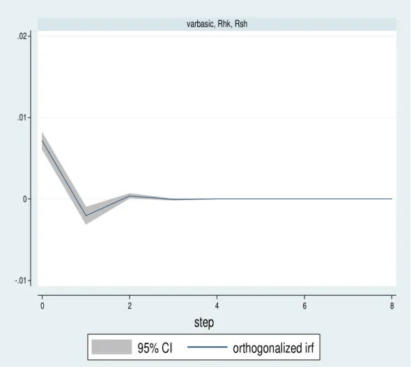
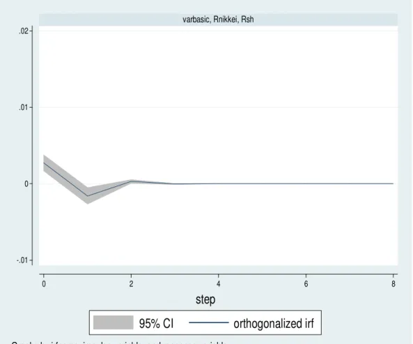
Impulse Response Analysis

Granger Causality test indicates that which variable could significant effect the other variables, however, Granger Causality could not test that how long the effect will take place. Impulse response analysis and forecast error variance decomposition may provide evidence that how long the effect will take place. Impulse response function shows the effects of shocks on the path of the variables.

Pesaran (1998) proposed impulse response analysis which tests the responsiveness of the dependent variables in the VAR model to shocks from the other variables. Impulse response function (IRF) of a dynamic system is its output when presented with a brief input signal, called an impulse. More generally, an impulse response refers to the reaction of any dynamic system in response to some external exchange. According to Pesaran (1998), the impulse response analysis quantifies the reaction of every single variable in the model on an exogenous shock to the model. There are two special cases of shocks can be identified: the single equation shock and the joint equation shock where the shock mirrors the residual covariance structure. In the first case we investigate forecast error impulse responses, in the second case orthogonalized impulse responses. The reaction is measured for every variable a certain time after shocking the system. The impulse response analysis is capable a tool for inspecting the inter-relation of the model variables. Therefore, when unit shock is applied to the error, the effects upon the VAR system over time will noted for every variable from equation.

(38)

So far, the pure mathematical techniques have been described. Since the purpose of this paper is looking for the relationship among international stock markets, the financial theory of market efficiency will be discussed next.

Chapter 4 Statistical Analysis and Results

Overall Practices

The data being examined in this study is daily return of the chosen indexes as mentioned before, from January 1st2007 to December 31st 2011. Within this period, all the holiday data are deleted; therefore, the left number of observations of each variable is 1113.

The code of Index is described below:

Country National Stock Index Name Abbreviation

China Shanghai Stock Exchange

Composite Index

United States NYSE Composite Index

Hong Kong Hang Seng Composite Index

Japan Nikkei 225 Stock Average

4.1 Descriptive Statistic Summary of each index

Before reporting the tests results, the past statistical data of these stock markets return is summarized first. Below are the descriptive statistical summaries of these national stock markets return that are chosen in this paper.

(39)

The following estimation is conducted based on a sample of daily return of four national stock indexes: Rsh, Rnyse, Rhk and Rnikkei. The sample period spans from 1st January of 2007 to 31st December of 2011. As demonstrated in the graphs, all series fluctuate around their means, there is no sign of time trends and drifts in all of time series lines.

Figure 4.1 -Time series Rsh (left hand side on the top), Rnyse (right top), Rhk (left bottom)

and Rnikkei (right bottom)

Summary of Descriptive Statistical Value

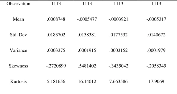
Figure 4.2- Basic descriptive statistics of all of time series

Index Return Rsh Rhk Rnyse Rnikkei

-. 1 -. 0 5 0 .0 5 .1 R s h

01jan2007 01jan2008 01jan2009 01jan2010 date -. 1 -. 0 5 0 .0 5 .1 R n y s e

01jan2007 01jan2008 01jan2009 01jan2010 date -. 1 -. 0 5 0 .0 5 .1 .1 5 R h k

01jan2007 01jan2008 01jan2009 01jan2010

date -. 1 -. 0 5 0 .0 5 .1 .1 5 R n ik k e i

01jan2007 01jan2008 01jan2009 01jan2010

(40)

Observation 1113 1113 1113 1113 Mean .0008748 -.0005477 -.0003921 -.0005317 Std. Dev .0183702 .0138381 .0177532 .0140672 Variance .0003375 .0001915 .0003152 .0001979 Skewness -.2720899 .5481402 -.3435042 -.2058349 Kurtosis 5.181656 16.14012 7.663586 17.9069

Stata 12 outputs are in Appendix

A.

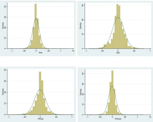
Figure 4.2 provides basic descriptive statistics of the four series. The mean returns of all of series are 0.0008748 for Rsh, -0.0005477 for Rhk, -0.0003921 for Rnyse and -0.0005317 for Rnikkei, with a standard deviation of 0.0183702, 0.0138381, 0.0177532 and 0.140672 respectively. Only Rhk seems to be positively skewed, and the other three are negatively skewed. Additionally, all of series demonstrate kurtosis above 3 which implies that more observations lie in the tail of the distributions. However, skewness and kurtosis do not seem to be a problem. A further test on skewness and kurtosis indicates that the skewness and kurtosis effects are jointly insignificant for all of series at the 5% significance level, which means that normality assumption in the following is valid. The histograms in figure 2 support this finding as they indicate that all series distributions follow a normal distribution quit well.

(41)

The correlation coefficient analysis

Since all the time series are normal distribution, Pearson correlation coefficient can be applied. In order to portray a general picture of the correlation among the international stock markets return, the table of the correlation coefficient is shown as below. This could give some information about the linkage among these national stock markets return.

Figure 4.4 -Pearson Correlation Coefficient

Correlation Coefficient Table

Rhk Rsh Rnyse Rnikkei Rhk 1 Rsh 0.4055 1 0 1 0 2 0 3 0 4 0 D e n s it y -.1 -.05 0 .05 .1 .15 Rhk 0 1 0 2 0 3 0 D e n s it y -.1 -.05 0 .05 .1 Rsh 0 1 0 2 0 3 0 4 0 D e n s it y -.1 -.05 0 .05 .1 Rnyse 0 1 0 2 0 3 0 4 0 D e n s it y -.1 -.05 0 .05 .1 .15 Rnikkei

(42)

(0.0000) Rnyse 0.3609 (0.0000) 0.0975* (0.0011) 1 Rnikkei 0.3372 (0.0000) 0.1622 (0.0000) 0.2118 (0.0000) 1

*Not significant at 5 percent level. N.B. Stata outputs are in Appendix B.

From the table above, the simple idea of correlation among these national indexes return may be obtained. It seems all of variables are positively and significantly correlated, except for Rnyse-Rsh pair. It may indicate that the international stock markets return is positively correlated in some degree level. As for Shanghai stock exchange composite index return, the correlation between Shanghai composite index daily return and Hang Seng composite index daily return is 0.4055, it may indicate that there is positive correlation between it and Hang Seng composite index while there is very low correlation between Shanghai stock market return and the United States stock market return since the correlation is 0.0975, also 0.0975 seems not significant at 5 percent level. The correlation coefficient between Chinese stock market and Japanese stock market is 0.1622, which is lower than correlation between Chinese stock market and Hong Kong stock market. It indicates that Chinese stock market is correlated with Hong Kong stock market most among international stock markets.

It also can be found both Japanese stock market and Hong Kong stock market are positive correlated with the United States market. The correlation coefficient between Japanese stock market and the United States market is 0.2118 and the correlation between Hong Kong stock market and Japanese stock market is 0.3372.

(43)

From this table, we may gain idea that correlation among these stock markets return. More specifically for Chinese stock market, it indicates that Hong Kong is most correlated with Shanghai stock market, and then Japanese stock market, the United States market. However, the correlation coefficient analyse cannot fully capture the property of a time series like the data of the stock index closing price. Hence, the time series techniques are applied next to explain to analyze the relationship among international stock market.

4.2 Unit root test

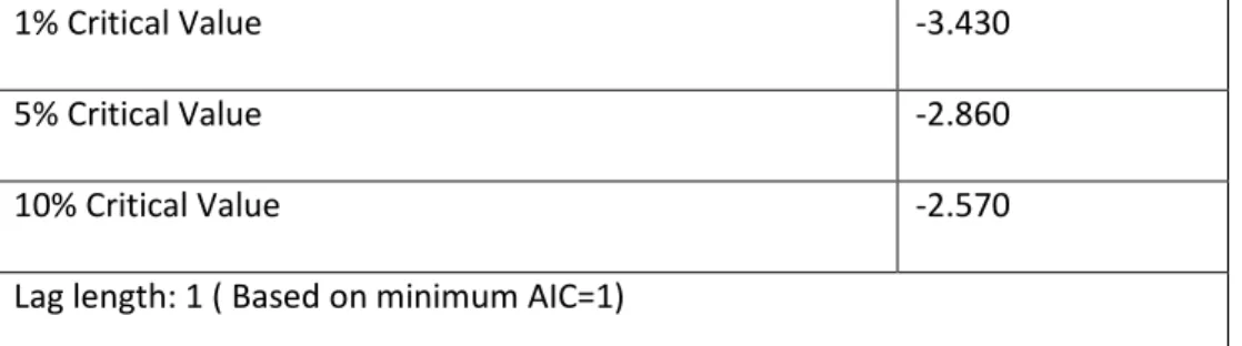
In order to test the property of stationary of the dataset, unit root is applied to test stationary. As discussed above, ADF test is a proper tool to test unit root. Before carrying out ADF test, the lag length should be selected first. Also, there are three forms of equation of ADF test, as discussed above, all of time series used in this paper fluctuate around their mean, there is no constant and drift in time series. Therefore, the ADF test is conducted without constant and trend term. In ADF test, the null hypothesis is that, the series has a unit root and thus is non-stationary.

According to Aikiake Information Criterion (AIC), the lag length of each viiable including SH, HK,NYSE and NIKKEI is 1,1,1,1.

Following are the Unit Root tests results of all single variables:

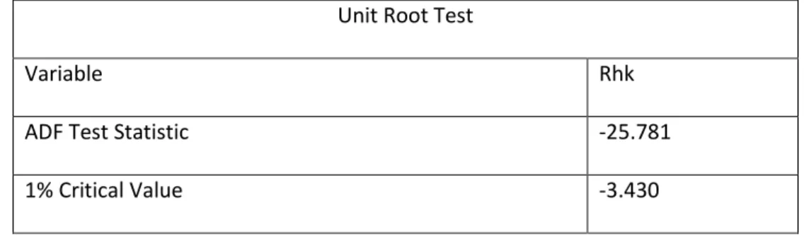
Figure 4.2a -Unit Root Test: Hang Seng Stock Exchange Composite Index

Unit Root Test

Variable Rhk

ADF Test Statistic -25.781

(44)

5% Critical Value -2.860

Lag length: 2 ( Based on minimum AIC=2)

Stata outputs are in Appendix C.

The test results showed that the variable Rhk is stationary. In the ADF test, the ADF statistic value is smaller than any critical value in any of significance level. Therefore, the null hypothesis is rejected, the Rhk variable is stationary.

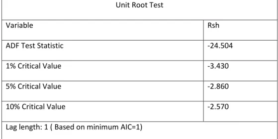
Figure 4.2b -Unit Root Test: Shanghai Stock Exchange Composite Index

Unit Root Test

Variable Rsh

Stata outputs are in Appendix D.

The test reults revealed that the variable Rsh is stationary. The ADF test statistic is smallerr than 1%, 5% and 10% and nonstationary null hypothesis is rejected at any level.

Figure 4.2c -Unit Root Test : New York Stock Exchange Composite Index

Unit Root Test

Variable Rnyse

(45)

Stata outputs are in Appendix E.

The test results revealed that the variable Rnyse is stationary. The ADF test statistic is -24.771 and smaller than 1%, 5% and 10% and nonstationary null hypothesis is rejected at any level.

Figure 4.2d -Unit Root Test : Nikkei 225 Stock Exchange Composite Index

Unit Root Test

Variable Rnikkei

Stata outputs are in Appendix F.

The test results suggested that the variable Rnikkei has no unit root . The null hypothesis is rejected at any level.

So far, the unit root tests have been done to test stationary. The results indicated that all of these variables are stationary. As mentioned before, these unstationary time series do not have to be translated to stationary time series. Therefore, these time series could be applied in next models.

(46)

4.3 Granger Causality test

From the pair-wise test of Granger Causality test, the cause-result relationship between variables may be obtained, that is, which variable plays the leading role between them. And another convenience which may be brought by conducting the Granger Causality test before applying the vector-regression (VAR) model is that, via this test, the ranking of the level of impact from the United States, Hong Kong and Japanese markets to Chinese market can be observed. Therefore, it will help to facilitate the following coamparasons and analyses adopted.

The Granger Causality test coulf only be applied to a stationary series. As discussed above, ADF test suggested that all series are stationary. In Granger Causality test, the null hypothesis is as shown in the table below. And here 5% significance level is adopted.

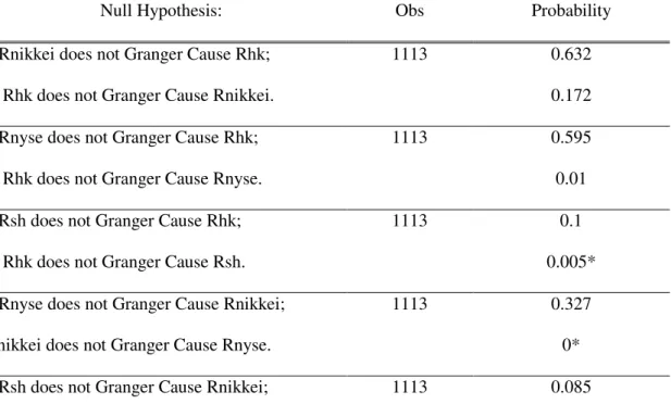
Figure 4.3a - Granger Causality Test

Lags:1 Sample: 1113

Null Hypothesis: Obs Probability 1.Rnikkei does not Granger Cause Rhk; 1113 0.632

Rhk does not Granger Cause Rnikkei. 0.172 2.Rnyse does not Granger Cause Rhk; 1113 0.595 Rhk does not Granger Cause Rnyse. 0.01 3.Rsh does not Granger Cause Rhk; 1113 0.1

Rhk does not Granger Cause Rsh. 0.005* 4.Rnyse does not Granger Cause Rnikkei; 1113 0.327 Rnikkei does not Granger Cause Rnyse. 0* 5.Rsh does not Granger Cause Rnikkei; 1113 0.085